Feasibility of Using Green Laser for Underwater Infrastructure Monitoring: Case Studies in South Florida

1
Department of Ocean and Mechanical Engineering, Florida Atlantic University, Boca Raton, FL 33431, USA
2
Department of Civil, Environmental and Geomatics Engineering, Florida Atlantic University, Boca Raton, FL 33431, USA
*
Author to whom correspondence should be addressed.
Geomatics 2024, 4(2), 173-188; https://doi.org/10.3390/geomatics4020010
Submission received: 2 March 2024
/
Revised: 26 April 2024
/
Accepted: 13 May 2024
/
Published: 17 May 2024
Abstract
:Scour around bridges present a severe threat to the stability of railroad and highway bridges. Scour needs to be monitored to prevent the bridges from becoming damaged. This research studies the feasibility of using green laser for monitoring the scour around candidate railroad and highway bridges. The laboratory experiments that provided the basis for using green laser for underwater mapping are also discussed. The results of the laboratory and field experiments demonstrate the feasibility of using green laser for underwater infrastructure monitoring with limitations on the turbidity of water that affects the penetrability of the laser. This method can be used for scour monitoring around offshore structures in shallow water as well as corrosion monitoring of bridges.
1. Introduction
Scour needs to be monitored in a timely manner as around 80% of the railroad and highway bridges in the US are built over water bodies [1,2]. Natural disasters like earthquakes associated with heavy rain and flooding can severely damage bridges [3]. Regular monitoring of bridges is needed to maintain the structural integrity of the railroad and highway bridges [4,5]. After the New York Thruway bridge collapsed in 1987, the Federal Highway Administration (FHWA) started its national bridge scour evaluation program under the National Bridge Inspection (NBI) [6]. Under this four-phase program, the hydrologic, geotechnical, and hydraulic data of the bridge are collected and assessed in detail. Based on the assessment, recommendations are suggested if the bridge is susceptible to scour. Over the years, various state Department of Transportations (DOTs) have developed maintenance requirements to monitor scour. Typically, this involves annual or biennial inspections performed by divers. However, the review after heavy rainfall or flood events is rare due to the exacerbation of scour, and the risks associated with manual scour measuring techniques. Scour around bridge piers are usually measured using in-contact and non-contact scour measuring devices. Some examples of in-contact sensors include float-out devices, tethered buried switches, piezoelectric sensors, buried rods, and radar devices [2,7]. A float-out device measures the scour when it is disconnected from the ground. A float-out device is kept near the bridge, which is equipped with electrical switch triggers. Once the scour extends to the bottom of the device, it will float on the surface of the water giving direct measurements of the scour [7,8]. The working principle of the tethered buried switch is the same as that of the float-out device [9]. The tethered buried switch changes its position from vertical to horizontal when the scour reaches the bottom of the device, triggering the electrical switch [7]. One of the main disadvantages of these devices (the float-out device and tethered buried switch) is that it does not measure maximum scour. The assistance of a diver is required for the installation of these devices [10,11]. The buried rod uses gravity sensors to measure the scour [12]. Scour-measuring buried rods are installed near the bridge pier. As the scour extends, the device moves along with the scour, giving scour dimensions. Measuring probes with radar devices measure the variation in the dielectric permittivity constant [13]. Probes are installed near bridge piers, and when the dielectric permittivity constant changes for the water and soil interface, scour is measured. Radar devices are also used for measuring bridge deflections [14]. The piezoelectric sensors measure the hydrodynamic forces of water on the sensor [9,15,16]. The sensor is installed on a cantilever near the bridge pier. When the scour starts to progress, bending forces are induced on the cantilever, which directly measures the scour. The piezoelectric sensor also needs the support of a diver for its installation.
In recent years, there has been a shift towards non-contact scour measuring equipment and this equipment does not require the support of a diver and can be operated without being in direct contact with the scour. Some of the non-contact scour measuring devices are GPR (Ground Penetrating Radar), SONAR (Sound Navigation and Ranging), echo sounder, seismic profiler, and laser devices [2,7]. GPR sends electromagnetic waves to the scour profile, which are reflected to the device [17], whereas SONAR uses sound-based ranging for underwater and scour mapping [2,7]. Sound waves sent by the SONAR device gets reflected from the scour hole, and its dimensions are measured [18,19]. High-frequency seismic pulse is used by seismic profiler for scour measurement, which is sent from the transducer and gets reflected from the scour profile to the receiver [2,17,20,21]. The working principle of an echosounder is the same as that of seismic profiler [22]. The echosounder sends a high-frequency acoustic pulse for scour mapping [2,13]. Laser devices most commonly use a green wavelength laser for scour measurement. Blue and infrared wavelengths are also used [23]. Since water absorbs the green laser least, it is mainly used for underwater operations. Refraction correction must be applied to the data collected by the green laser to extract the dimensions of the scour [24]. The green laser can be used with fixed and floating stations. Unmanned Aerial Vehicles (UAVs), ships, barges, etc., can be mounted with the green laser for scour measurements [2].
Yagci et al., 2017 used green laser to measure the scour near the hexagonal arrangement of circular piers [23]. The flow conditions used for the experiments were steady. The Leica Scan station C10 is used for experimental study. The cylinders were arranged in regular, angled, and staggered configurations. The green laser was found to be effective in mapping scour around cylinders. When the cylinders are arranged in regular configuration, the generated scour is less than angled and staggered configurations. Poggi & Kudryavtseva, 2019 used cyan line laser to measure the scour in the front and behind the bridge pier [25]. The wavelength of the cyan line laser used was 488 nm. A glass cylinder with a diameter of 3.2 cm made up of Plexiglass was used as a bridge pier. The experiments were carried out in a 12 m long flume. The flow in the flume was regulated using a hydraulic gate. The highest scour depth from the laser scan was compared with the highest scour depth obtained from Oliveto & Hager, 2002 [26] and Melville and Chiew, 1999 [27]. The scour mapping using the cyan line laser successfully maps the scour near the bridge pier. Musab, 2018 used green laser and hydrolite SONAR to demonstrate its feasibility in scour mapping [28]. The Leica Scan Station II was used for the green laser mapping. A 6.6-inch diameter circular PVC (Polyvinyl Chloride) pipe was used as a bridge pier, and a prefabricated scour hole was set around the PVC pipe. The experimental setup was installed in a frustum-shaped tank. The green laser scanning and hydrolite SONAR mapping were carried out for clear water conditions. The green laser could travel from the scan station through the air and water medium for scour mapping. The hydrolite SONAR was kept on the water surface for mapping the scour. The results from the feasibility study show that the green laser scan data had better resolution and higher magnitude. This is due to dense point cloud data collected from the green laser scan. At the same time, the SONAR scan data showed discrete elevated data points. The green laser captured the edges of the prefabricated scour hole more than the hydrolite SONAR. Raju et al., 2022 [2] continued the feasibility study of Musab, 2018 [28] by varying the turbidity conditions of the water and slightly changing the dimensions of the prefabricated scour hole [29,30]. The experimental studies were carried out in a pool with a diameter of 3.048 m. Two parameters were varied in the experiments—water depth and turbidity of water. The water depth range used was 0.38 to 0.6 m for turbidity levels ranging from 1.2 to 20.8 NTU (Nephelometric Turbidity Unit). Kaolinite powder was used to change water turbidity levels. The scour mapping was carried out by using a Leica Scan Station II, which uses green laser with 532 nm wavelength, and the accuracy of the green laser used is 4 mm [2]. The results from the underwater scan data were compared with the dry scan data of the prefabricated scour hole. The experimental study results show that water turbidity and water depth play an important role in the scour mapping using green laser.
The benefit of using green laser is that it can penetrate through the turbid water to the scour hole and gives a complete view of the scour hole. The scour monitoring using green laser can be performed from a stationary platform in land or from an aerial platform. These scans can be performed without the help of an underwater diver, which is not possible especially during high flood times. Based on the laboratory testing, the green laser was used for the feasibility study of scour mapping around candidate railroad and highway bridges in South Florida, which is discussed here. The railroad bridge selected for the study is the SXG59.70 railroad bridge near SW 112th St, Miami, FL, USA and the first highway bridge selected for the study was the Little Lake Worth bridge near 11072–11078 Florida A1A, Palm Beach Gardens, FL, USA. The second highway bridge selected for the study was the SX.928 located in the SW Warfield Blvd Road (FL-710), Indiantown, FL, USA. Based on the feasibility study of scour measurement around railroad and highway bridges, it was concluded that turbidity plays a significant role in the efficiency of green laser in underwater mapping.
2. Materials and Methods
The research methodology involves data collection using green wavelength Leica laser scanner and performing refraction correction using an in-house developed MATLAB routine. The laser scanner computes 3D geometric information namely X, Y, Z coordinates and reflectance of the scene using known azimuth and zenith angles and the computed range. The relationship can be expressed using a simple cartesian coordinates to polar coordinates transformation. The visualization and extraction of the laser point cloud were performed using Leica Cyclone (version 6.0.4) and Cloud Compare (version 2.12) software packages. Figure 1 shows the schematic diagram of the converted polar coordinates.
Refraction correction is applied to the X, Y, Z coordinates. “The X, Y, Z coordinates after refraction correction are shown in Equations (1)–(3) below [2]:
where (Xr, Yr, Zr) are the coordinates after refraction correction, ϕw = azimuth of the laser pulse, ϴw = refraction angle, Zw = height of water surface from scanner eyepiece, ϴa = incident angle of laser pulse”.
Xr = Rr sin ϕw
Yr = Rr cos ϕw
2.1. Laboratory Testing
Initially, the feasibility of using the green laser in scour monitoring was carried out in the laboratory using a prefabricated scour hole in a pool with diameter 3.048 m (Figure 2 and Figure 3) [2]. The turbidity inside the pool is changed from 1.2 to 20.8 NTU by adding Kaolinite powder. The turbidity of the clear water was 1.2 NTU. The turbidities considered for the study were 1.2 NTU, 3.9 NTU, 5.5 NTU, 6.4 NTU, 12.1 NTU, and 20.8 NTU. The fabricated scour model used in Nagarajan et al., 2018 and Banhany 2018 was used for laboratory experiments [2,24,28]. Six trials were conducted by varying the water depth of the pool. The scanning was carried out using the Leica Scan Station II. The water depth inside the pool was varied from 0.38 to 0.6 m.
Initially, the prefabricated scour hole was dry scanned to obtain a reference model for calibration. The dry scan of the prefabricated scour model was used as a reference model to compare the scan data for different turbidity levels and water depths. The scour mapping was carried out by mixing kaolinite powder with pool water to increase the turbidity [2]. Based on the underwater scan, the depth of water was decreased when the underwater scan of the prefabricated scour hole was not completely visible. The underwater scan was carried out for turbidity levels up to 20.8 NTU. For turbidity 20.8 NTU, the depth near the prefabricated scour hole was 0.2 m, and 0.3 m elsewhere in the pool. The green laser undergoes refraction underwater and refraction correction was applied to the scan data. Figure 4 and Figure 5 show the sample scan for a turbidity level of 5.5 NTU before and after applying refraction correction.
The laboratory experiments showed the green laser is effective in underwater mapping. As the turbidity of water in the pool was increased, the edges of the prefabricated scour hole became less visible even after the depth of water was decreased.
2.2. Field Testing
Based on the laboratory testing, the green laser was used for a feasibility study of scour mapping around one railroad bridge and two highway bridges in South Florida, United States. Figure 6 shows the location of all the bridges considered here in this study for the underwater scan using green laser. The railroad bridge selected for the study is the SXG59.70 railroad bridge near SW 112th St, Miami, Florida, United States. The average turbidity of the water samples collected from the canal’s surface is 0.45 NTU. The pictorial view and the approximate dimensions of the SXG59.70 railroad bridge are shown in Figure 7 and Figure 8. Figure 9 and Figure 10 show the scan station on the right and left banks of the canal near the railroad bridge.
The first highway bridge selected for the study was the Little Lake Worth bridge near 11072–11078 Florida A1A, Palm Beach Gardens, FL, USA (Figure 11). The Florida Department of Transportation (FDOT) owns and maintains the bridge. The bridge’s approximate dimensions are shown in Figure 12.
Water samples were collected during the scanning process from different locations around the highway bridge piers. The average turbidity of the water samples collected from the surface was 1.74 NTU. For underwater scanning, an ASPEN A-62 Bridge Inspection snooper truck was used (Figure 13). The snooper truck is owned by the Florida Department of Transportation District 4 office located in Fort Lauderdale, Florida, United States. The Leica Scan Station II with the tripod was set up in the man basket of the snooper truck (Figure 14).
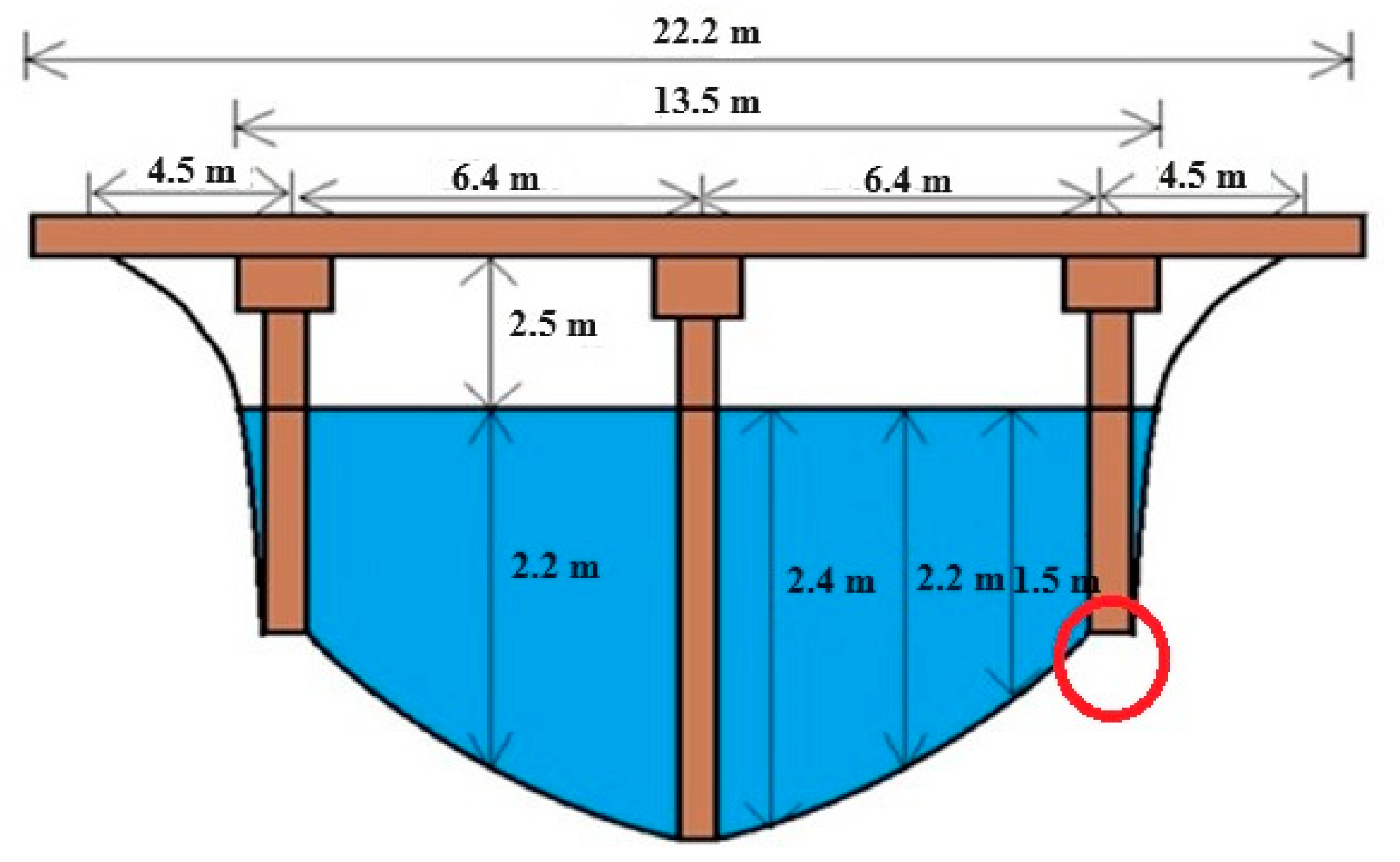
The second highway bridge selected for the study was the SX.928 located in the SW Warfield Blvd Road (FL-710), Indiantown, FL, USA. The bridge is owned and maintained by the Florida Department of Transportation. The water under the bridge was highly turbid and the water depth under the bridge was 0.28 m. Water samples were collected to measure the average turbidity of the water and the turbidity was 5.25 NTU. Figure 15 shows the Leica scan station II set up for underwater scanning of SX.928 highway bridge. The approximate dimensions of the bridge are shown in Figure 16.
3. Results and Discussions
The first underwater scan was performed for the SXG59.70 railroad bridge. The scan stations were set up on both banks of the canal. The scan was carried out for the right end (in red circle) of the pier using two scan stations on the two banks of the canal (Figure 17). Figure 18 shows the point cloud data collected from the right bank of the canal (station 1), and Figure 19 shows the point cloud data collected from the left bank of the canal (station 2). Figure 20, Figure 21 and Figure 22 show the point cloud data before and after the refraction correction.
From Figure 20, Figure 21 and Figure 22, the green laser was unable to reach the bottom of the bridge pier due to high water turbidity in the canal. The bottom of the canal was highly turbid, and the green laser could not reach the bottom of the canal.
The underwater scan was performed for the bridges using the green laser. For the highway bridge, laser scanning was performed using the help of a snooper truck.
The scan was carried out for the left end pier (in red circle) using the Leica Scan Station in the man basket (Figure 23). With the help of the snooper truck, the man basket could be moved around various locations. The man basket was able to be moved around different locations, and scan data was collected when the man basket was stationary. Figure 24 and Figure 25 show the scan data of the left end pier.
Since there was constant boat traffic under the bridge, the water on the top surface was disturbed continuously (Figure 26). The underwater scan data of the left end pier was collected effectively. The laser was undergoing refraction while traveling through the water, and refraction correction was carried out for the data points collected. Figure 27 shows the point cloud data before and after refraction correction.
From the point cloud data, it is visible that there is no visible scour around the left end pier. The green laser is effective in underwater scanning around the bridge pier. The scan data around other piers were not able to be obtained as there was continuous boat traffic.
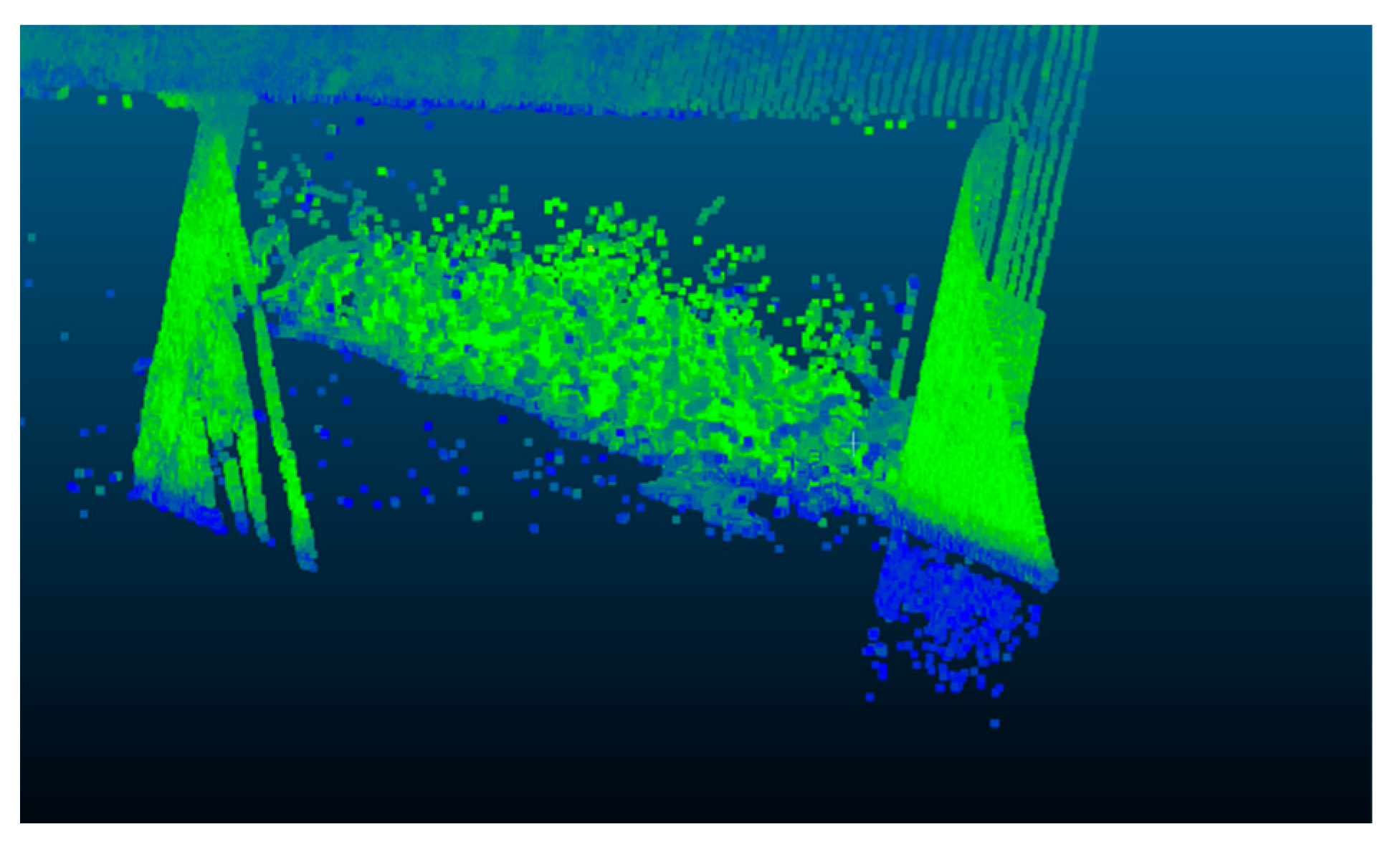
The final scan was carried out for the center pier and right end (shown in red circle) of the SX.928 highway bridge using the Leica Scan Station II (Figure 28). Figure 29 shows the point cloud data from the scan. The green laser was unable to reach the bottom of the highway bridge due to highly turbid water. The scattering of the laser was also high for this case.
4. Conclusions
The feasibility study was carried out using the green laser to examine scour around one railroad bridge and two highway bridges in South Florida, USA. The railroad bridge selected was the SXG59.70 railroad bridge near SW 112th St, Miami, Florida, United States. The highway bridges selected were the Little Lake Worth bridge near 11072–11078 Florida A1A, Palm Beach Gardens, Florida, and the SX.928 bridge located in the SW Warfield Blvd Road (FL-710), Indiantown, FL, USA. The feasibility study was carried out based on laboratory studies conducted on a prefabricated scour hole in a pool with diameter 3.048 m. The turbidity inside the pool was changed by adding Kaolinite powder. The turbidity inside the pool was changed from 1.2 to 20.8 NTU. When the green laser travels from air to water, the laser undergoes refraction and refraction correction was applied to the collected data points. The minimum range, maximum range, reflectance, and point density play an important role in underwater scanning [2]. The incident angle of the green laser plays an important role in the underwater scanning. The green laser has the advantage of penetrating through the turbid water and gives a complete view of the scour hole. Based on the water samples collected from different locations around the railroad and highway bridge piers, the average turbidity of water for the railroad bridge was 0.45 NTU and for the highway bridges were 1.74 and 5.25 NTU. The underwater scan was carried for the right end pier of the SXG59.70 railroad bridge from the banks of the canal using the Leica Scan Station II. The green laser was unable to reach the bottom of the bridge pier due to high water turbidity in the canal. Since the bottom of the canal was highly turbid, the green laser could not reach the bottom of the canal. The underwater scanning using the green laser extended to the Little Lake Worth and SX.928 highway bridges. An underwater scan was carried out for the left end pier of the Little Lake Worth bridge with the help of an ASPEN A-62 Bridge Inspection snooper truck. The underwater scan data of the left end pier was collected effectively. Underwater scans around other piers of Little Lake Worth bridge were not able to be performed due to highly turbid water created by continuous boat traffic. The final scan was carried out for the center pier and right end of the SX.928 highway bridge. The green laser was not able to reach the bottom of the highway bridge due to highly turbid water. Based on the feasibility study of scour measurement around railroad and highway bridges, it was concluded that turbidity plays a significant role in the efficiency of green laser in underwater mapping. Turbidity should be measured at different locations of the water body. Green laser mapping is an effective method for scour monitoring and mapping since it is a non-contact method of scour monitoring. Scour monitoring using the green laser can be used for monitoring scour around bridge piers made up of concrete, steel, wood, etc. [32,33]. Bridge pier corrosion can be monitored using the green laser [34] and can be used for bathymetry profiling [35,36,37] and the detection of underwater objects [2]. The scour around the offshore structures like gravity-based, monopile, tripod, and suction bucket type structures in shallow water can also be monitored using green laser [33,38,39].
Author Contributions
Conceptualization, R.D.R., S.N., M.A. and S.C.; methodology, R.D.R., S.N., M.A. and S.C.; software, S.N. and R.D.R.; validation, S.N. and R.D.R.; formal analysis, R.D.R., S.N. and S.C.; investigation, R.D.R., S.N., M.A. and S.C.; resources, R.D.R., S.N., M.A. and S.C.; data curation, R.D.R., S.N. and S.C; writing—original draft preparation, R.D.R.; writing—review and editing, R.D.R. and S.N.; visualization, S.N.; supervision, S.N. and M.A.; project administration, S.N.; funding acquisition, S.N. All authors have read and agreed to the published version of the manuscript.
Funding
National Academies of Sciences, Engineering & Medicine (Grant number—SAFETY-39) and Transportation Research Board’s Rail Safety IDEA Program (Grant number—BDV27-977-16), jointly funded this project.
Institutional Review Board Statement
Not applicable.
Informed Consent Statement
Not applicable.
Data Availability Statement
Limited data are contained within the article.
Acknowledgments
CSX Transportation and Florida Department of Transportation (FDOT) are acknowledged by the authors for their immense support. Also, authors would like to thank Transportation Research Board (TRB), USA and FDOT, USA for granting permission to use data from the reports of project for preparing this paper.
Conflicts of Interest
The authors declare no conflicts of interest. The funders had no role in the design of the study; in the collection, analyses, interpretation of data; or in the writing of the manuscript. The funders gave consent to publish data from the reports of project.
References
- Browne, T.M.; Collins, T.J.; Garlich, M.J.; O’Leary, J.E.; Stromberg, D.G.; Heringhaus, K.C. Underwater Bridge Inspection (No. FHWA-NHI-10-027); Federal Highway Administration, Office of Bridge Technology: Washington, DC, USA, 2010.
- Raju, R.D.; Nagarajan, S.; Arockiasamy, M.; Castillo, S. Feasibility of Using Green Laser in Monitoring Local Scour around Bridge Pier. Geomatics 2022, 2, 355–369. [Google Scholar] [CrossRef]
- Vargas Neumann, J.; Sosa Cárdenas, C.; Montoya Robles, J. Stone Bags Seismic Isolation for Vernacular Earth and Stone Construction. In Structural Analysis of Historical Constructions: An Interdisciplinary Approach; Springer International Publishing: Cham, Switzerland, 2019; pp. 1528–1536. [Google Scholar]
- Javed, A.; Sadeghnejad, A.; Yakel, A.; Azizinamini, A. Magnetic Flux Leakage (MFL) Method for Damage Detection in Internal Post-Tensioning Tendons; Final Report, FDOT Contract No. BDV29-977-45; Florida International University: Miami, FL, USA, 2021. [Google Scholar]
- Hameed, A.; Rasool, A.M.; Ibrahim, Y.E.; Afzal, M.F.U.D.; Qazi, A.U.; Hameed, I. Utilization of Fly Ash as a Viscosity-Modifying Agent to Produce Cost-Effective, Self-Compacting Concrete: A Sustainable Solution. Sustainability 2022, 14, 11559. [Google Scholar] [CrossRef]
- Lagasse, P.F.; Richardson, E.V.; Weldon, K.E. Florida Department of Transportation Bridge Scour Evaluation Program. In Proceedings of the Fourth International Bridge Engineering Conference, San Francisco, CA, USA, 28–30 August 1995; Transportation Research Board Conference Proceedings. Transportation Research Board: Washington, DC, USA, 1995. [Google Scholar]
- Prendergast, L.J.; Gavin, K. A review of bridge scour monitoring techniques. J. Rock Mech. Geotech. Eng. 2014, 6, 138–149. [Google Scholar] [CrossRef]
- Whitehouse, R.J.; Sutherland, J.; Harris, J.M. Evaluating scour at marine gravity foundations. Proc. Inst. Civ. Eng.-Marit. Eng. 2011, 164, 143–157. [Google Scholar] [CrossRef]
- Prendergast, L.J. Monitoring of bridge scour using changes in natural frequency of vibration-a field investigation. In Proceedings of the 5th International Young Geotechnical Engineer’s Conference, Paris, France, 31 August–1 September 2013; IOS Press: Amsterdam, The Netherland, 2013. [Google Scholar]
- Yao, C.; Darby, C.; Hurlebaus, S.; Price, G.R.; Sharma, H.; Hunt, B.E.; Yu, O.-Y.; Chang, K.-A.; Briaud, J.-L. Scour Monitoring Development for Two Bridges in Texas. In Proceedings of the International Conference on Scour and Erosion (ICSE-5) 2010, San Francisco, CA, USA, 7–10 November 2010; pp. 958–967. [Google Scholar]
- Briaud, J.L.; Hurlebaus, S.; Chang, K.A.; Yao, C.; Sharma, H.; Yu, O.Y.; Darby, C.; Hunt, B.E.; Price, G.R. Realtime Monitoring of Bridge Scour Using Remote Monitoring Technology; No. Report 0-6060-1; Texas Transportation Institute: College Station, TX, USA, 2011.
- Lagasse, P.F.; Richardson, E.V.; Schall, J.D. Fixed Instrumentation for Monitoring Scour at Bridges. Transp. Res. Rec. 1998, 1647, 1–9. [Google Scholar] [CrossRef]
- Fisher, M.; Atamturktur, S.; Khan, A.A. A novel vibration-based monitoring technique for bridge pier and abutment scour. Struct. Health Monit. 2013, 12, 114–125. [Google Scholar] [CrossRef]
- Afzal MF, U.D.; Matsumoto, Y.; Nohmi, H.; Sakai, S.; Su, D.; Nagayama, T. Comparison of Radar Based Displacement Measurement Systems with Conventional Systems in Vibration Measurements at a Cable Stayed Bridge. In Proceedings of the 11th German-Japan Bridge Symposium, Osaka, Japan, 30–31 August 2016. [Google Scholar]
- Lin, Y.-B.; Chen, J.-C.; Chang, K.-C.; Chern, J.-C.; Lai, J.-S. Real-time monitoring of local scour by using fiber Bragg grating sensors. Smart Mater. Struct. 2005, 14, 664–670. [Google Scholar] [CrossRef]
- Kong, X.; Ho, S.C.M.; Song, G.; Cai, C.S. Scour Monitoring System Using Fiber Bragg Grating Sensors and Water-Swellable Polymers. J. Bridg. Eng. 2017, 22, 04017029. [Google Scholar] [CrossRef]
- Anderson, N.L.; Ismael, A.M.; Thitimakorn, T. Ground-Penetrating Radar: A Tool for Monitoring Bridge Scour. Environ. Eng. Geosci. 2007, 13, 1–10. [Google Scholar] [CrossRef]
- Deng, L.; Cai, C.S. Bridge scour: Prediction, modeling, monitoring, and countermeasures. Pract. Period. Struct. Des. Constr. 2010, 15, 125–134. [Google Scholar] [CrossRef]
- Schall, J.D. Sonar Scour Monitor: Installation, Operation, and Fabrication Manual; Transportation Research Board: Washington, DC, USA, 1997. [Google Scholar]
- Placzek, G. Surface-Geophysical Techniques Used to Detect Existing and Infilled Scour Holes Near Bridge Piers; No. 4009; US Department of the Interior, US Geological Survey: Reston, VA, USA, 1995; Volume 95.
- Webb, D.J.; Anderson, N.L.; Newton, T.; Cardimona, S. Bridge scour: Application of ground penetrating radar. In Proceedings of the First International Conference on the Application of Geophysical Methodologies and NDT to Transportation Facilities and Infrastructure, St. Louis, MO, USA, 11–15 December 2000; Federal Highway Commission and Missouri Department of Transportation: St. Louis, MO, USA, 2000. [Google Scholar]
- Porter, K.; Simons, R.; Harris, J. Comparison of three techniques for scour depth measurement: Photogrammetry, echosounder profiling and a calibrated pile. Coast. Eng. Proc. 2014, 34, 64. [Google Scholar] [CrossRef]
- Yagci, O.; Yildirim, I.; Celik, M.F.; Kitsikoudis, V.; Duran, Z.; Kirca, V.O. Clear water scour around a finite array of cylinders. Appl. Ocean Res. 2017, 68, 114–129. [Google Scholar] [CrossRef]
- Nagarajan, S.; Arockiasamy, M.; Banyhany, M. Bridge Pier Scour Hole Simulation and 3D Reconstruction Using Green Laser (No. 18-05495). In Proceedings of the Compendium of Transportation Research Board 97th Annual Meeting, Washington, DC, USA, 7–11 January 2018. [Google Scholar]
- Poggi, D.; Kudryavtseva, N.O. Non-Intrusive Underwater Measurement of Local Scour Around a Bridge Pier. Water 2019, 11, 2063. [Google Scholar] [CrossRef]
- Oliveto, G.; Hager, W.H. Temporal Evolution of Clear-Water Pier and Abutment Scour. J. Hydraul. Eng. 2002, 128, 811–820. [Google Scholar] [CrossRef]
- Melville, B.W.; Chiew, Y.-M. Time Scale for Local Scour at Bridge Piers. J. Hydraul. Eng. 1999, 125, 59–65. [Google Scholar] [CrossRef]
- Banyhany, M. 3D Reconstruction of Simulated Bridge Pier Local Scour Using Green Laser and Hydrolite Sonar. Master’s Thesis, Atlantic University, Boca Raton, FL, USA, 2018. [Google Scholar]
- Nagarajan, S.; Arockiasamy, M. Non-Contact Scour Monitoring for Highway Bridges; Repository and Open Science Access Portal, National Transportation Library: Washington, DC, USA, 2020.
- Nagarajan, S.; Arockiasamy, M. Non-Contact Scour Monitoring System for Railroad Bridges; No. Rail Safety IDEA Project 39; Transportation Research Board: Washington, DC, USA, 2020. [Google Scholar]
- Smith, M.; Vericat, D.; Gibbins, C. Through-water terrestrial laser scanning of gravel beds at the patch scale. Earth Surf. Process. Landforms 2011, 37, 411–421. [Google Scholar] [CrossRef]
- Cardenas, C.S.; Mantawy, I.M.; Azizinamini, A. Repair of Timber Piles Using Ultra-High-Performance Concrete: Investigation of Load Transfer and Load-Carrying Capacity. Transp. Res. Rec. 2023, 2677, 1016–1032. [Google Scholar] [CrossRef]
- Arockiasamy, M.; Arvan, P.A. Behavior, Performance, and Evaluation of Prestressed Concrete/Steel Pipe/Steel H-Pile to Pile Cap Connections. Pr. Period. Struct. Des. Constr. 2022, 27, 03122001. [Google Scholar] [CrossRef]
- Rehmat, S.; Sadeghnejad, A.; Javed, A. Automated MFL System for Corrosion Detection; Florida International University: Miami, FL, USA, 2021. [Google Scholar]
- Yang, F.; Su, D.; Yue, M.; Feng, C.; Yang, A.; Wang, M. Refraction correction of airborne LiDAR bathymetry based on sea surface profile and ray tracing. IEEE Trans. Geosci. Remote Sens. 2017, 55, 6141–6149. [Google Scholar] [CrossRef]
- Roman, C.; Inglis, G.; Rutter, J. Application of structured light imaging for high resolution mapping of underwater archaeological sites. In Proceedings of the OCEANS’10 IEEE SYDNEY, Sydney, NSW, Australia, 24–27 May 2010; IEEE: Piscataway, NJ, USA, 2010; pp. 1–9. [Google Scholar]
- Szafarczyk, A.; Toś, C. The Use of Green Laser in LiDAR Bathymetry: State of the Art and Recent Advancements. Sensors 2023, 23, 292. [Google Scholar] [CrossRef] [PubMed]
- Arvan, P.A.; Raju, R.D.; Arockiasamy, M. Offshore Wind Turbine Monopile Foundation Systems in Multilayered Soil Strata under Aerodynamic and Hydrodynamic Loads: State-of-the-Art Review. Pr. Period. Struct. Des. Constr. 2023, 28, 03123001. [Google Scholar] [CrossRef]
- Guan, D.-W.; Xie, Y.-X.; Yao, Z.-S.; Chiew, Y.-M.; Zhang, J.-S.; Zheng, J.-H. Local scour at offshore windfarm monopile foundations: A review. Water Sci. Eng. 2021, 15, 29–39. [Google Scholar] [CrossRef]
Figure 1.
Schematic diagram of refraction correction applied for underwater scanning [adapted from Smith et al., 2012] [2,24,31].
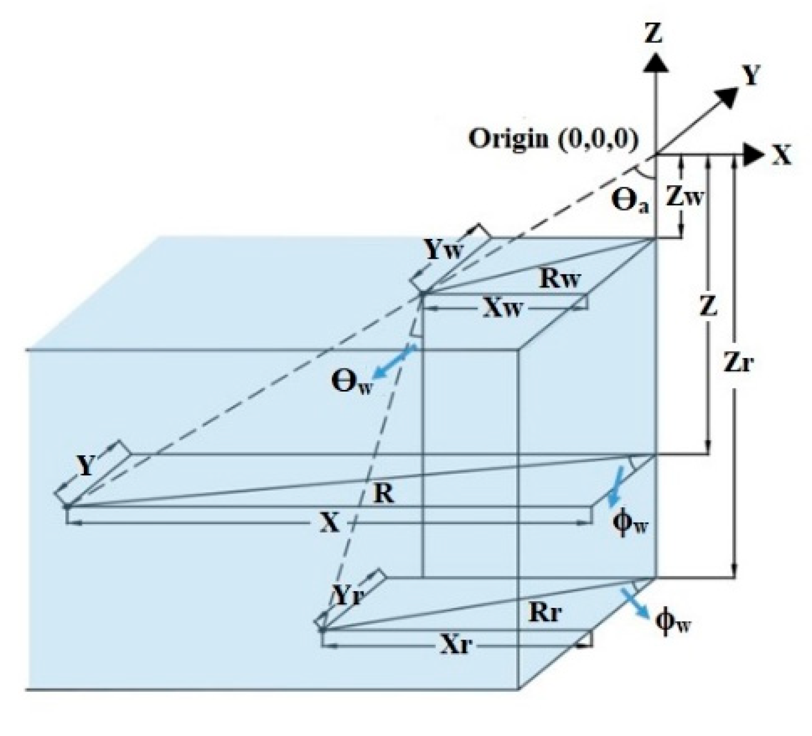


Figure 4.
Three-dimensional laser scan prior to refraction correction for turbidity 5.5 NTU [29] (used with permission).
Figure 4.
Three-dimensional laser scan prior to refraction correction for turbidity 5.5 NTU [29] (used with permission).

Figure 5.
Three-dimensional laser scan following the refraction correction for turbidity 5.5 NTU [29] (used with permission).
Figure 5.
Three-dimensional laser scan following the refraction correction for turbidity 5.5 NTU [29] (used with permission).
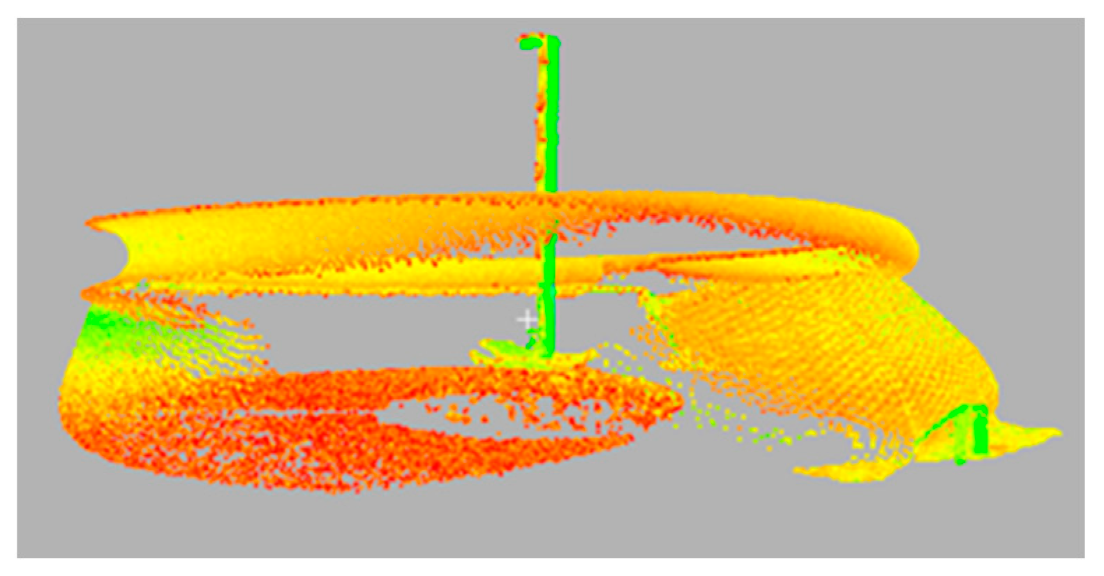
Figure 6.
Location of all the bridges considered for the study.
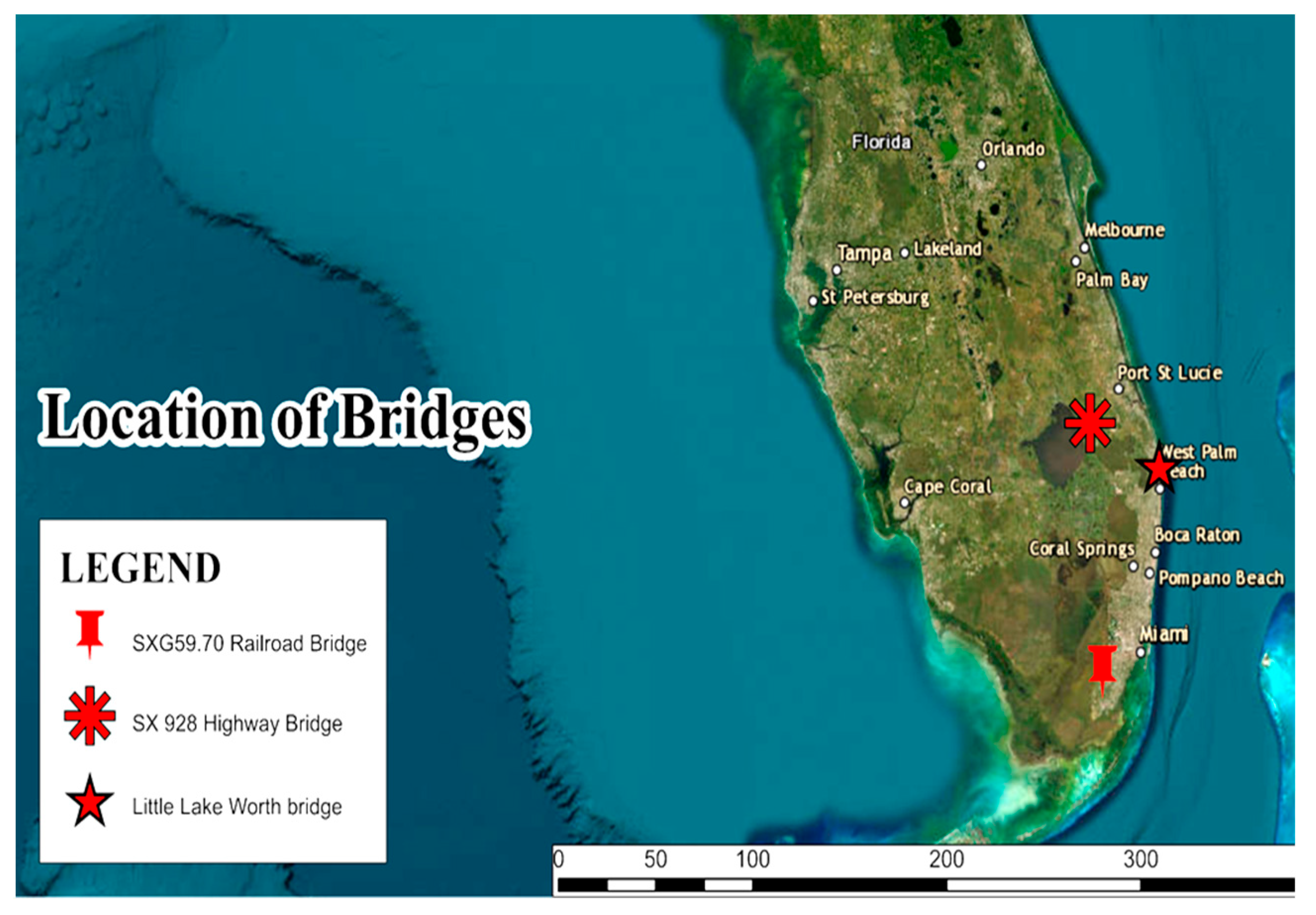
Figure 7.
Pictorial view of the railroad bridge—Miami, Florida.
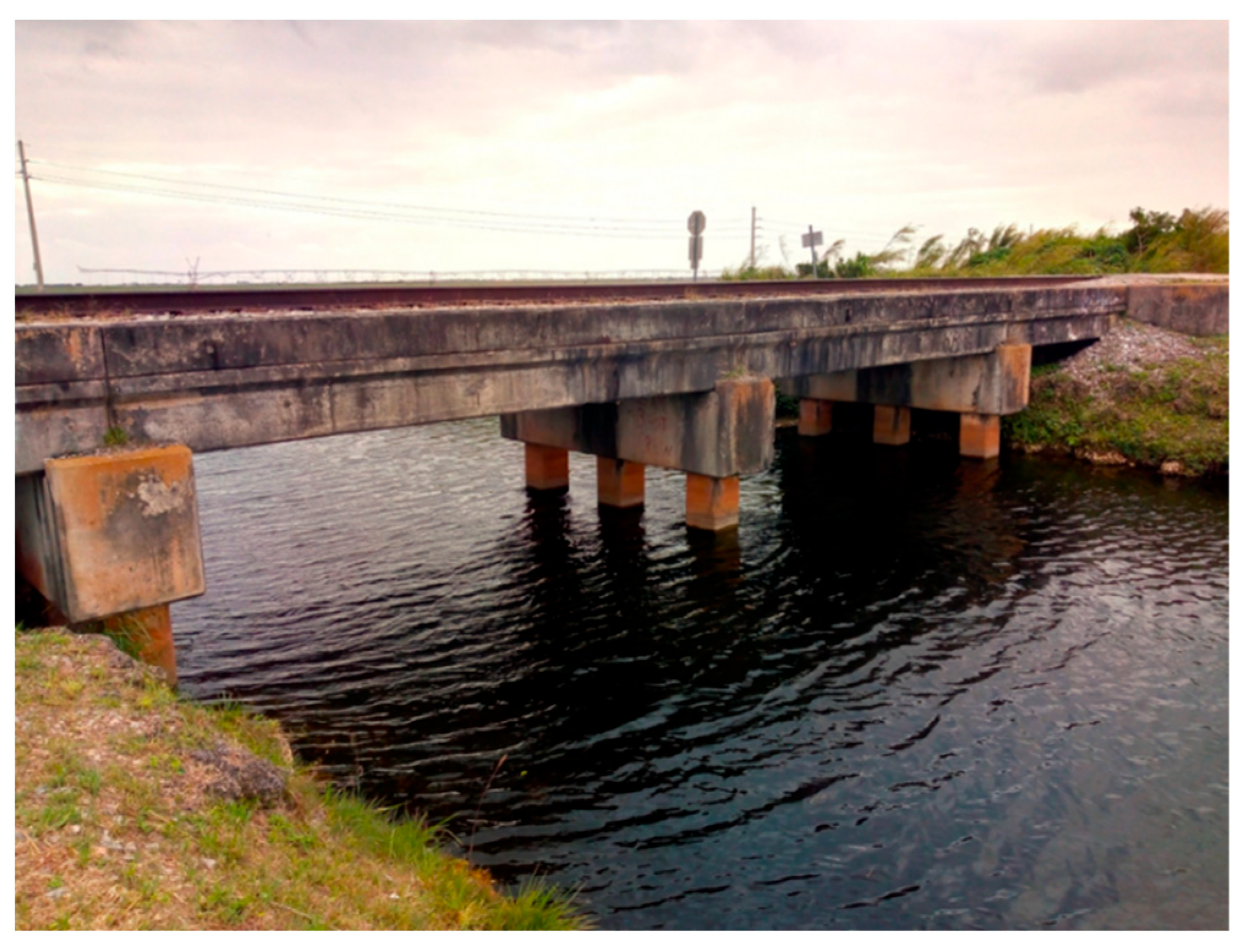
Figure 8.
Dimensions of the railroad bridge—Miami, Florida (approximate) [29,30] (used with permission).

Figure 9.
Scan station 1 set up on the right bank of the canal near the railroad bridge.
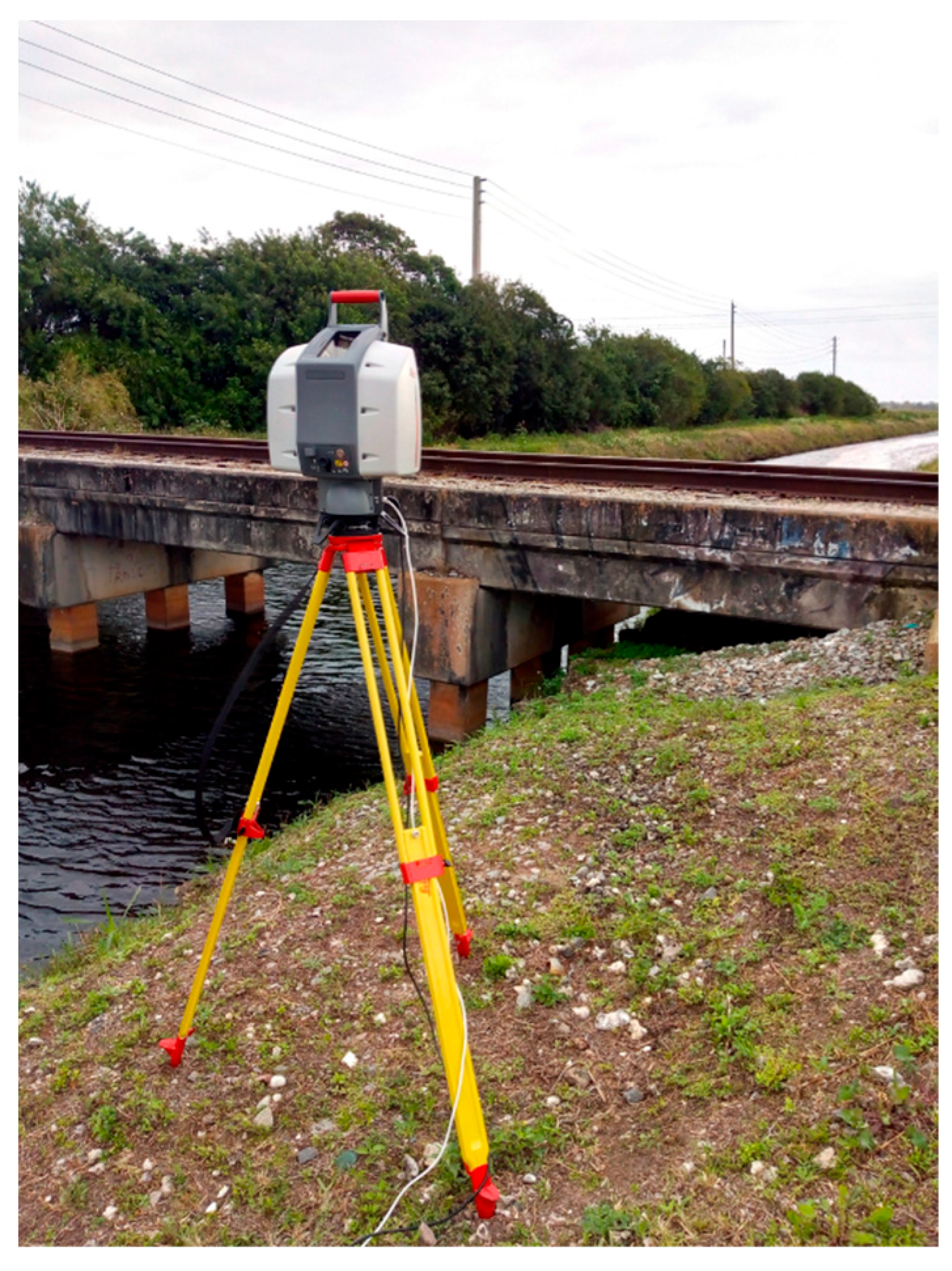
Figure 10.
Scan station 2 set up on the left bank of the canal near the railroad bridge.
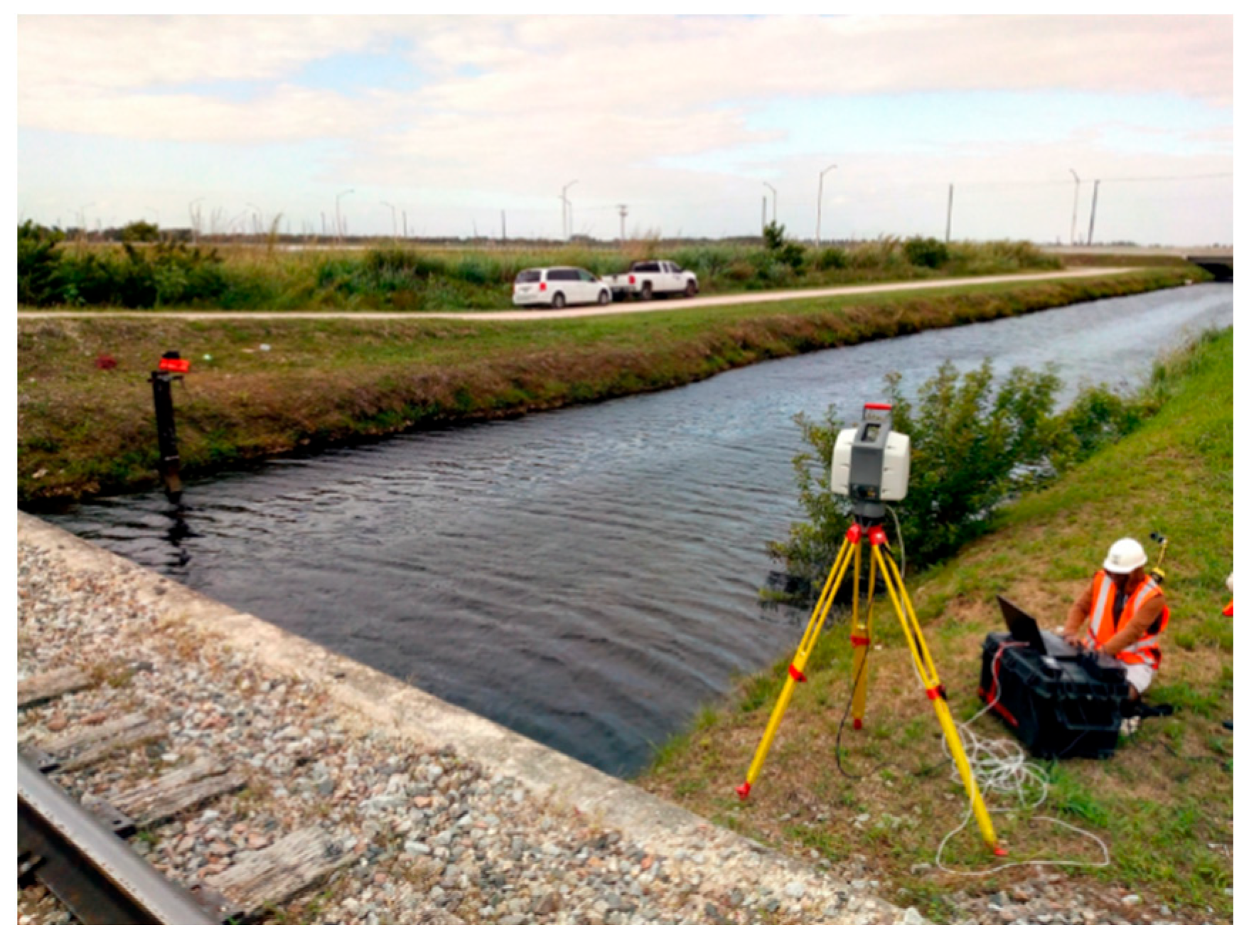
Figure 11.
Pictorial view of the highway bridge—Little Lake Worth bridge, Florida [29,30] (used with permission).
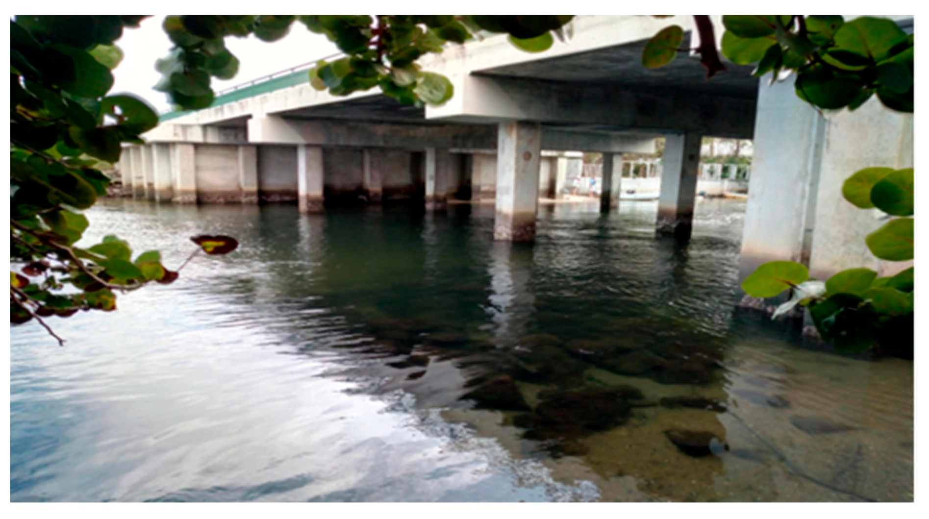
Figure 12.
Dimensions of the highway bridge (approximate)—Little Lake Worth Bridge, Florida [29,30] (used with permission).

Figure 13.
Snooper truck used for underwater scanning of highway bridge—Little Lake Worth Bridge, Florida.
Figure 13.
Snooper truck used for underwater scanning of highway bridge—Little Lake Worth Bridge, Florida.
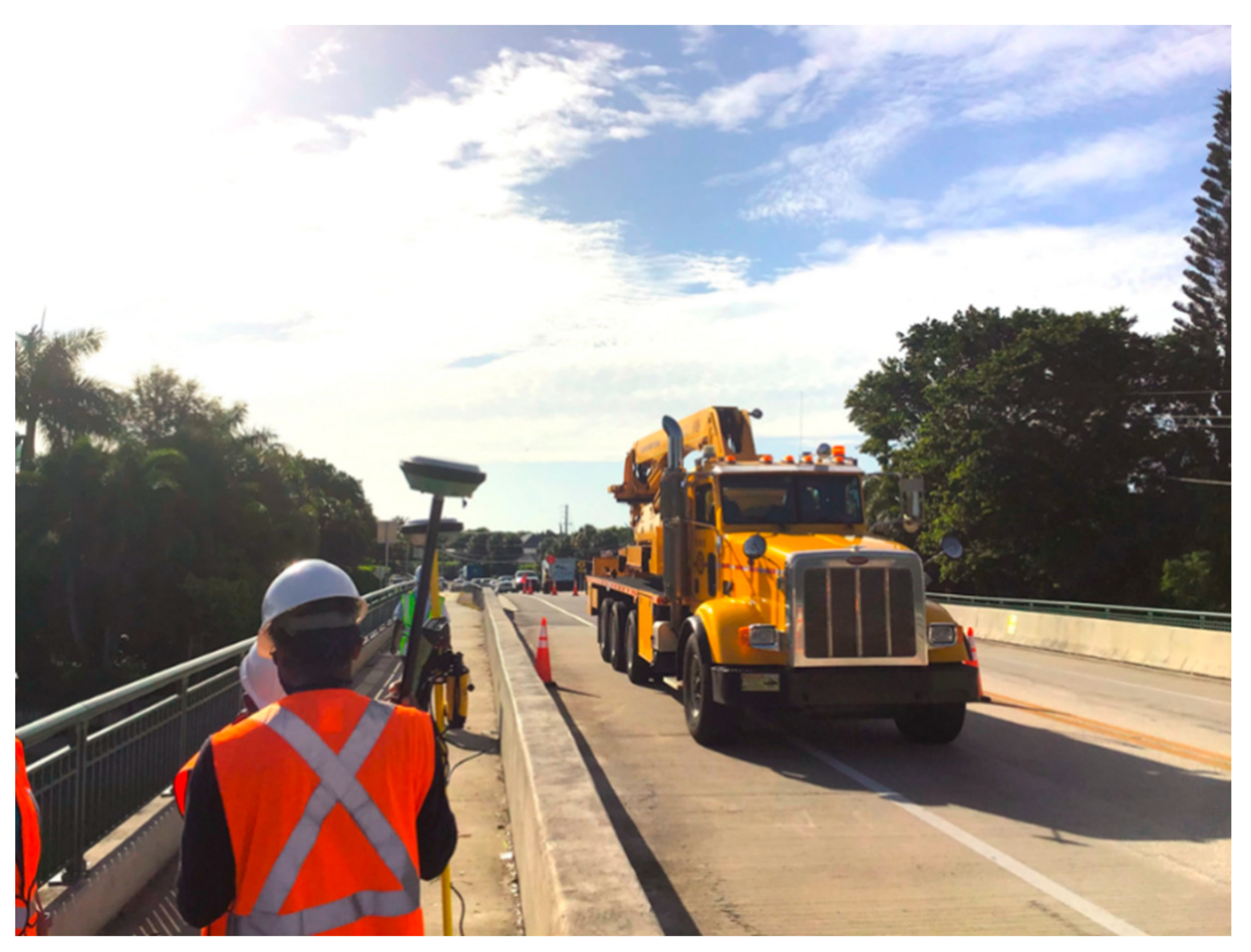
Figure 14.
Leica scan station II set up in man basket of snooper truck used for underwater scanning of highway bridge—Little Lake Worth Bridge, Florida.
Figure 14.
Leica scan station II set up in man basket of snooper truck used for underwater scanning of highway bridge—Little Lake Worth Bridge, Florida.
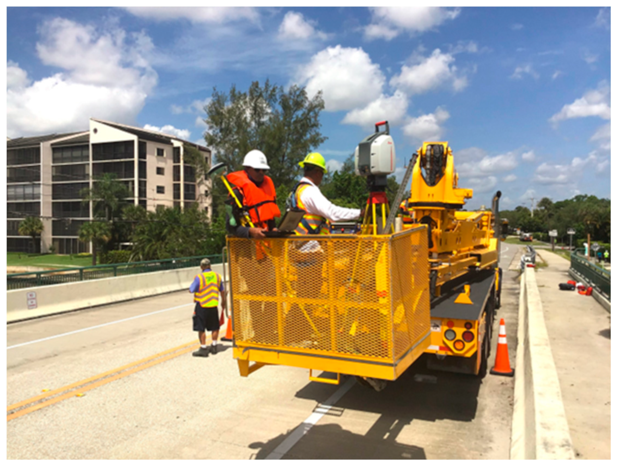
Figure 15.
Leica scan station II set up for underwater scanning of SX.928 highway bridge.
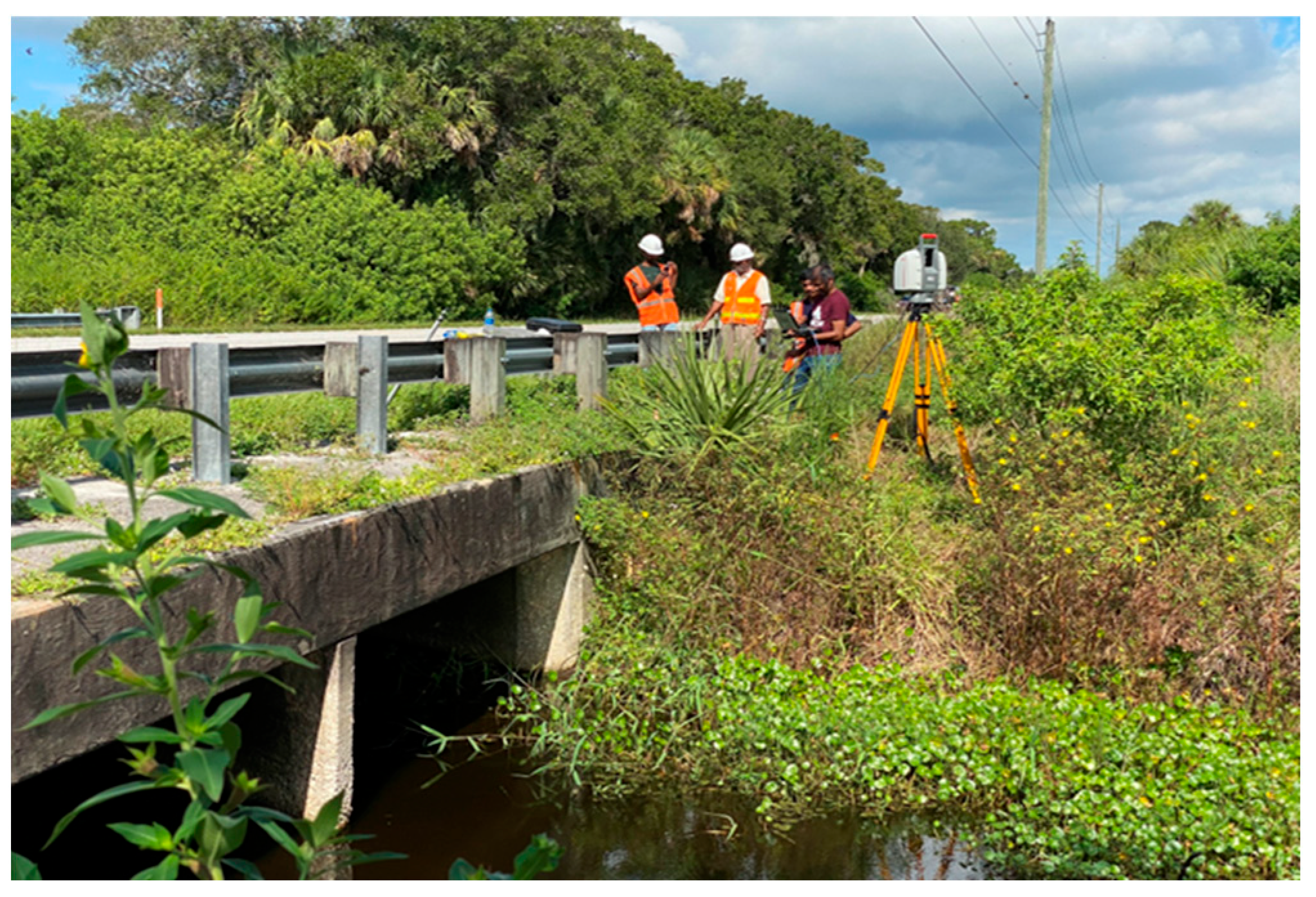
Figure 16.
Dimensions of the SX.928 highway bridge (approximate).

Figure 17.
Dimensions of the railroad bridge with targeted end pier in red circle—Miami, Florida [29,30] (used with permission).


Figure 20.
Railroad bridge green laser point cloud data before refraction correction [29,30] (used with permission).

Figure 21.
Railroad bridge green laser point cloud data from station 1 before (green) and after (white) refraction correction [29,30] (used with permission).
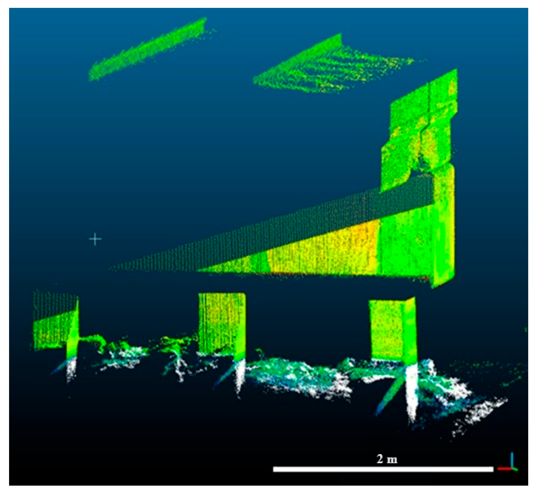
Figure 22.
Railroad bridge green laser point cloud data from station 2 before and after (white) refraction correction [29,30] (used with permission).

Figure 23.
Dimensions of the highway bridge with targeted end pier in red circle—Little Lake Worth, Florida [29,30] (used with permission).
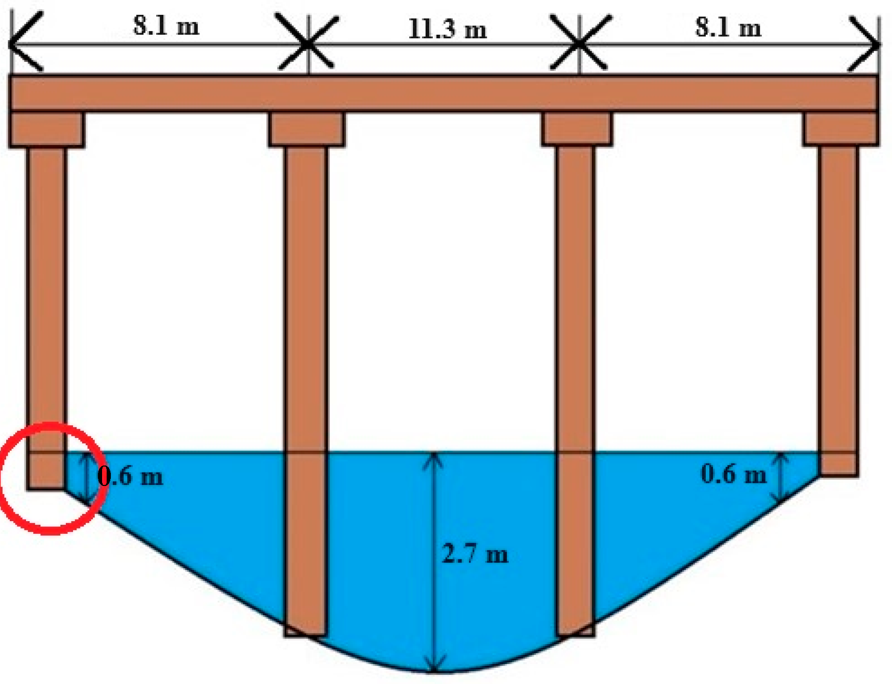
Figure 24.
Scan data of the end pier of the highway bridge, Little Lake Worth, Florida (display by hue intensity) [29,30] (used with permission).

Figure 25.
Scan data of the end pier of the highway bridge, Little Lake Worth, Florida (display by intensity) [29] (used with permission).
Figure 25.
Scan data of the end pier of the highway bridge, Little Lake Worth, Florida (display by intensity) [29] (used with permission).
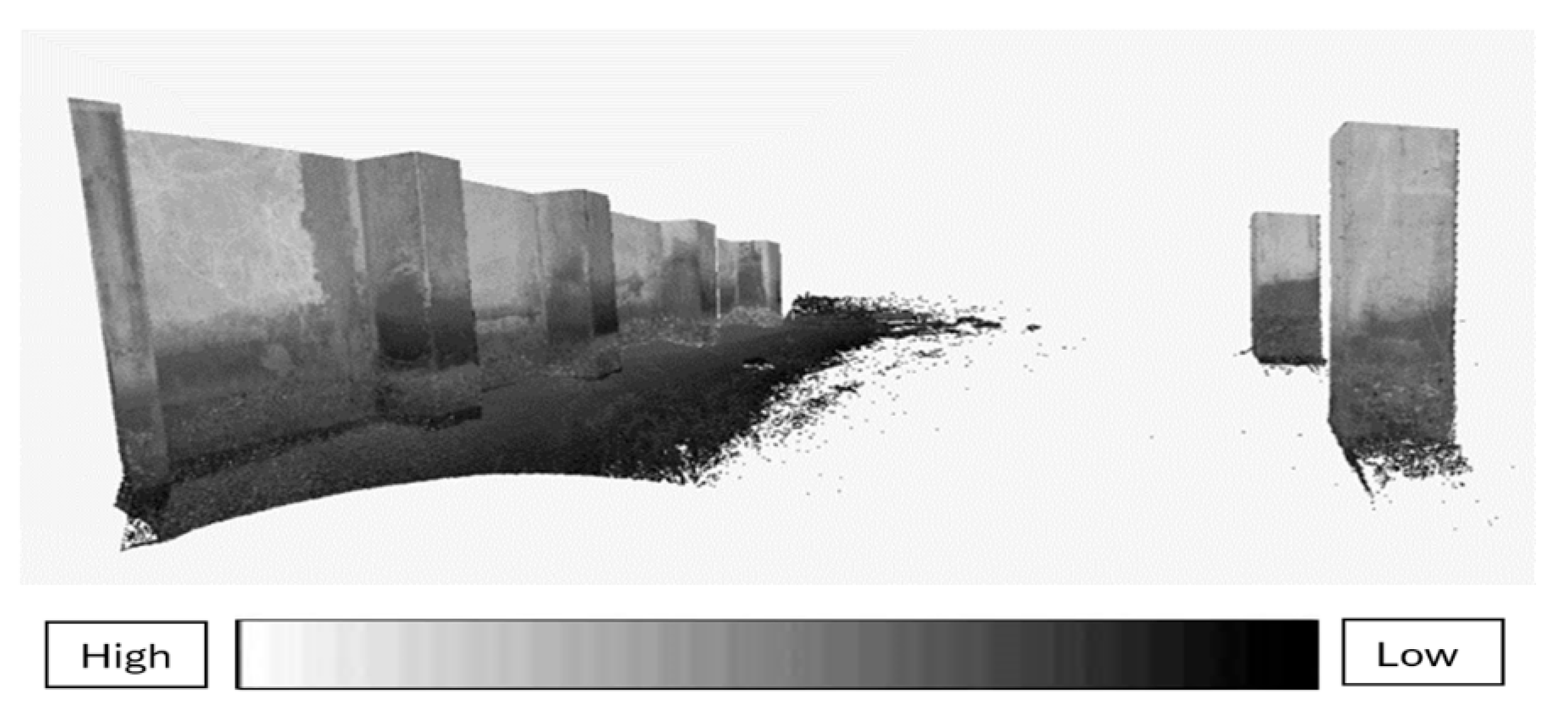
Figure 26.
Boat traffic under the highway bridge, Little Lake Worth, Florida.
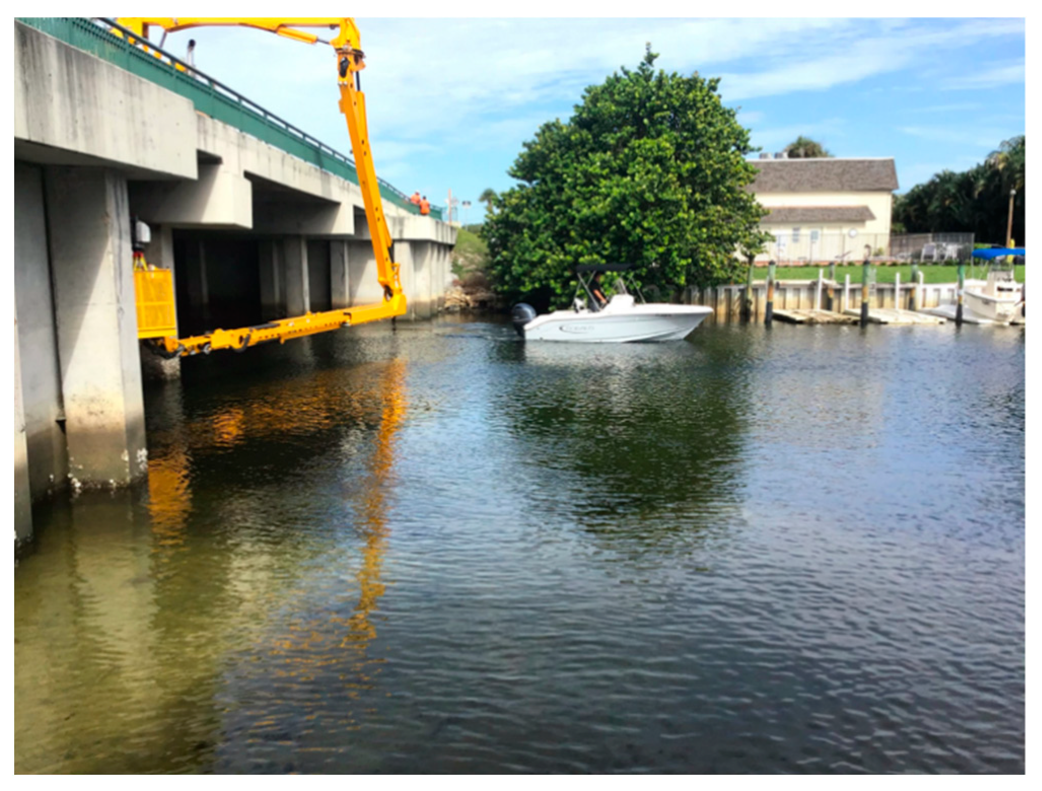
Figure 27.
Point cloud data before (green) and after (white) refraction correction of the left end pier—Little Lake Worth, Florida [29,30] (used with permission).
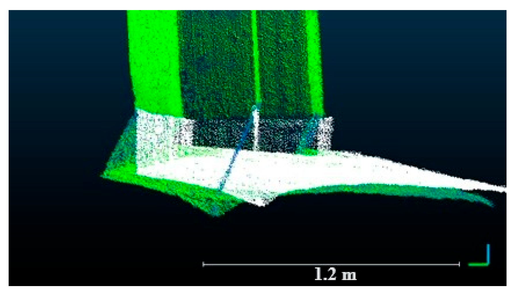
Figure 28.
Dimensions of the SX.928 highway bridge with targeted scan areas in red circle.
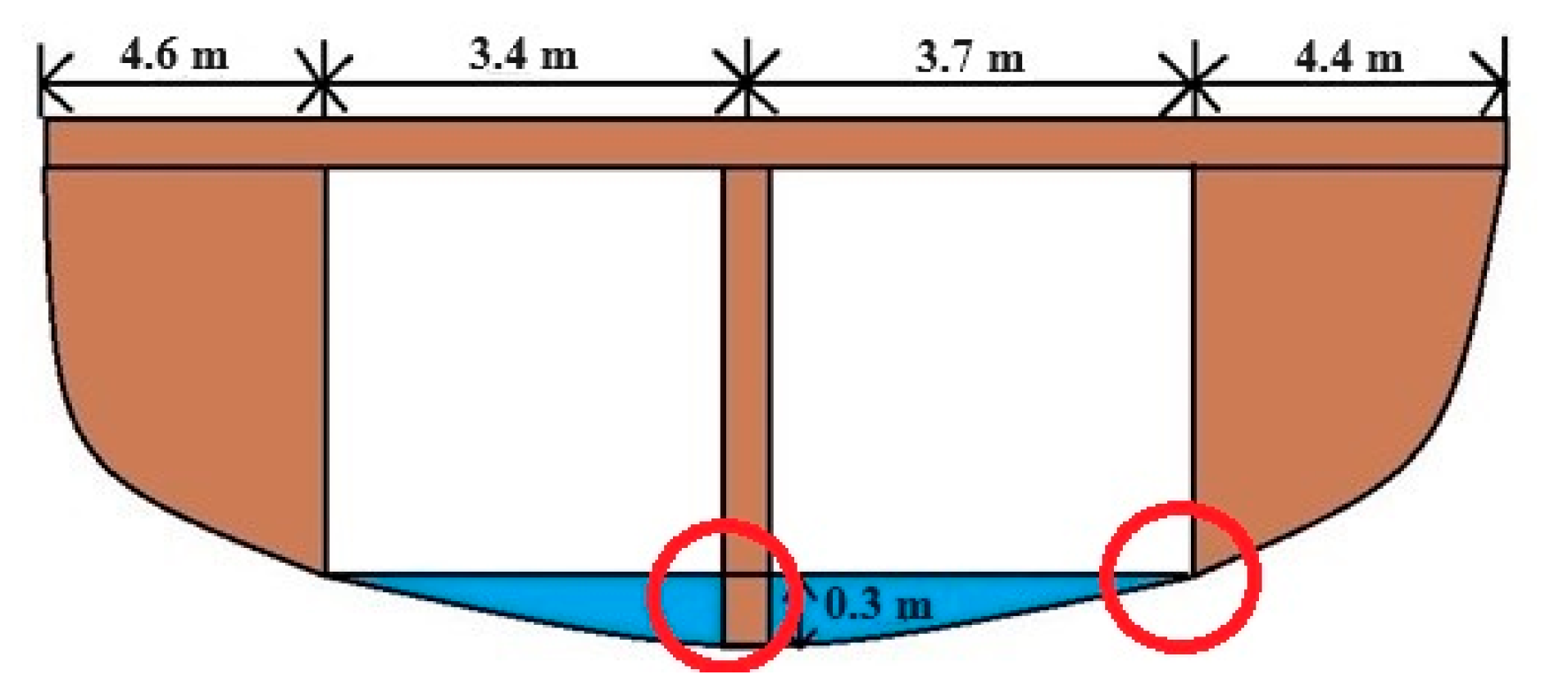
Figure 29.
Point cloud data from the laser scan for SX.928 highway bridge.
Disclaimer/Publisher’s Note: The statements, opinions and data contained in all publications are solely those of the individual author(s) and contributor(s) and not of MDPI and/or the editor(s). MDPI and/or the editor(s) disclaim responsibility for any injury to people or property resulting from any ideas, methods, instructions or products referred to in the content. |
© 2024 by the authors. Licensee MDPI, Basel, Switzerland. This article is an open access article distributed under the terms and conditions of the Creative Commons Attribution (CC BY) license (https://creativecommons.org/licenses/by/4.0/).
Share and Cite
MDPI and ACS Style
Raju, R.D.; Nagarajan, S.; Arockiasamy, M.; Castillo, S. Feasibility of Using Green Laser for Underwater Infrastructure Monitoring: Case Studies in South Florida. Geomatics 2024, 4, 173-188. https://doi.org/10.3390/geomatics4020010
AMA Style
Raju RD, Nagarajan S, Arockiasamy M, Castillo S. Feasibility of Using Green Laser for Underwater Infrastructure Monitoring: Case Studies in South Florida. Geomatics. 2024; 4(2):173-188. https://doi.org/10.3390/geomatics4020010
Chicago/Turabian StyleRaju, Rahul Dev, Sudhagar Nagarajan, Madasamy Arockiasamy, and Stephen Castillo. 2024. "Feasibility of Using Green Laser for Underwater Infrastructure Monitoring: Case Studies in South Florida" Geomatics 4, no. 2: 173-188. https://doi.org/10.3390/geomatics4020010