Article

Predictive Potential of Maize Yield in the Mesoregions of Northeast Brazil

by
Fabrício Daniel dos Santos Silva
1,
Ivens Coelho Peixoto
1,
Rafaela Lisboa Costa
1,
Helber Barros Gomes
1,
Heliofábio Barros Gomes
1,
Jório Bezerra Cabral Júnior
2,
Rodrigo Martins de Araújo
1 and
Dirceu Luís Herdies
3,*
1
Institute of Atmospheric Sciences, Federal University of Alagoas, Maceió 57072-900, Brazil
2
Institute of Geography, Development and Environment, Federal University of Alagoas, Maceió 57072-900, Brazil
3
National Institute for Space Research, Cachoeira Paulista, São Paulo 12630-000, Brazil
*
Author to whom correspondence should be addressed.
AgriEngineering 2024, 6(2), 881-907; https://doi.org/10.3390/agriengineering6020051
Submission received: 5 February 2024 / Revised: 15 March 2024 / Accepted: 25 March 2024 / Published: 2 April 2024

Abstract

:
Most of the northeastern region of Brazil (NEB) has a maize production system based on family farming, with no technological advances and totally dependent on the natural rainfall regime, which is concentrated in 4 to 5 months in most parts of the region. This means that the productivity of this crop is low in the NEB. In the northern mesoregions of the NEB, rainfall is concentrated between January and June, in the east of the NEB from April to September, and in the west of the NEB from October to March. The growing season takes place during these semesters. With this in mind, our objective was to develop a model based on canonical correlation analysis (CCA) to predict corn production in the mesoregions of the NEB between 1981 and 2010, using accumulated precipitation per semester as the predictor variable and predicting the observed production in kg/ha. Our results showed that the CCA model presented higher correlations between observed and simulated production than that obtained simply from the direct relationship between accumulated rainfall and production. The other two metrics used, RMSE and NRMSE, showed that, on average, in most mesoregions, the simulation error was around 200 kg/ha, but the accuracy was predominantly moderate, around 29% in most mesoregions, with values below 20% in six mesoregions, indicative of better model accuracy, and above 50% in two mesoregions, indicative of low accuracy. In addition, we investigated how the different combinations between two modes of climate variability with a direct influence on precipitation in the NEB impacted production in these 30 years, with the combination of El Niño and a positive Atlantic dipole being the most damaging to harvests, while years when La Niña and a negative Atlantic dipole acted together were the most favorable. Despite the satisfactory results and the practical applicability of the model developed, it should be noted that the use of only one predictor, rainfall, is a limiting factor for better model simulations since other meteorological variables and non-climatic factors have a significant impact on crops. However, the simplicity of the model and the promising results could help agricultural managers make decisions in all the states that make up the NEB.

1. Introduction

Every year, Brazil consolidates its position as one of the world’s leading grain producers, especially of soybeans and maize. According to CONAB (the national supply company responsible for monitoring and estimating Brazilian agricultural production), the grain harvest for the 2019/2020 season was 102.3 million tons [1], while for the 2023/2024 harvest, the estimate is 312.3 million tons of grain [2]. These figures show the average annual evolution of Brazilian grain production.
Maize stands out in this production scenario, giving Brazil third place in the world in the production of this grain, with approximately 12% of world production, behind only the United States (30% of world production) and China (24% of world production). Maize is essential in the production of biofuels [3], as well as being the staple food for billions of people around the world. It contains vitamins A and B, proteins, fats, carbohydrates, calcium, iron, phosphorus, and starch [4]. In Brazil, this cereal is also the main component used in the production of animal supplementation, destined for one of the main segments of Brazilian exports, which is the animal protein production chain [5,6].
Despite the high productivity of some Brazilian regions and their prominent role in world maize production, in the Northeast of Brazil (NEB), most mesoregions still grow maize through subsistence farming, with little or no mechanization and low technological potential. According to Garnett and Khandekar [7], the socio-economic impact on production is more intense in areas where there are major changes in climatic conditions, so it is understood that production varies considerably from year to year, which is the case in the NEB [8].
Water is a crucial factor in the development of the maize plant, the deficit of which is one of the main causes of a drop in productivity [9]. The need for water, temperature, and solar radiation are variables that directly affect the growth period, which reaches its maximum when these variables are optimally available, making it easier for the crop to reach its maximum yield capacity. In tropical conditions, according to the smaller variation in temperature and day length, the distribution of rainfall generally determines the best sowing time [10].
Maize consumes, on average, 400 to 700 mm of water in its complete cycle, depending on climatic conditions. Its period of maximum water demand occurs during the formation and filling of grains, that being the period in which water deficit causes the greatest reduction in its productivity [9]. Temperature is the main regulator of maize phenology, determining the emergence of seedlings and the rate of appearance of new leaves. Furthermore, the ideal soil temperature during the germination period is between 25 °C and 30 °C, with temperatures below 10 °C and above 40 °C being harmful to germination. Knowing that the ideal average environmental temperature for emergence and flowering is between 24 °C and 30 °C [11,12,13,14], in terms of this variable, the NEB as a whole contemplates the crop’s thermal needs, since its average annual temperature varies between 20 °C and 28 °C, with a variation from 24 °C to 26 °C in areas located above 200 m of altitude, and below 20 °C in elevated areas of Chapada Diamantina and Planalto da Borborema [15,16].
In the NEB, the high interannual variability of rainfall, climatically concentrated in a few months and marked by spatio-temporal variation, makes farming a high-risk activity, often doomed to total crop losses or low productivity [17]. Climate change scenarios for the region, with a decrease in accumulated rainfall and an increase in evapotranspiration, inspire even more concern for future yields [18]. Between 2012 and 2018, the NEB went through one of its longest droughts, both in terms of duration, magnitude, and intensity [19,20,21,22,23]. Medeiros et al. [24] showed that indices of climatic extremes indicate a reduction in rainfall in much of the Northeast in recent decades, and Pontes Filho et al. [25] showed that all areas of the NEB are highly susceptible to the return of droughts on different scales.
In regions, like the NEB, which are directly dependent on rainfall variability, the intensity of the loss associated with the harvest is greater, the greater is the shortage of rainfall. In this way, a useful tool for decision-making processes in agriculture would be a good crop forecast based on a prediction of the accumulated rainfall during the crop’s growing season. In this sense, the innovative nature of this research is to analyze the predictive potential of maize crop productivity in all the mesoregions of the NEB through the relationship between historical productivity and accumulated rainfall in the rainy semester, using the multivariate analysis technique Canonical Correlation Analysis (CCA). With this, we sought to correlate and identify the periods of greatest influence of rainfall on maize productivity in the mesoregions of the NEB, calibrate a crop forecasting model based on CCA, and also quantify the influence of the two main modes of climate variability that affect the distribution of rainfall in the mesoregions of the NEB, ENOS and the Atlantic dipole, and their respective impacts on maize productivity.

2. Materials and Methods

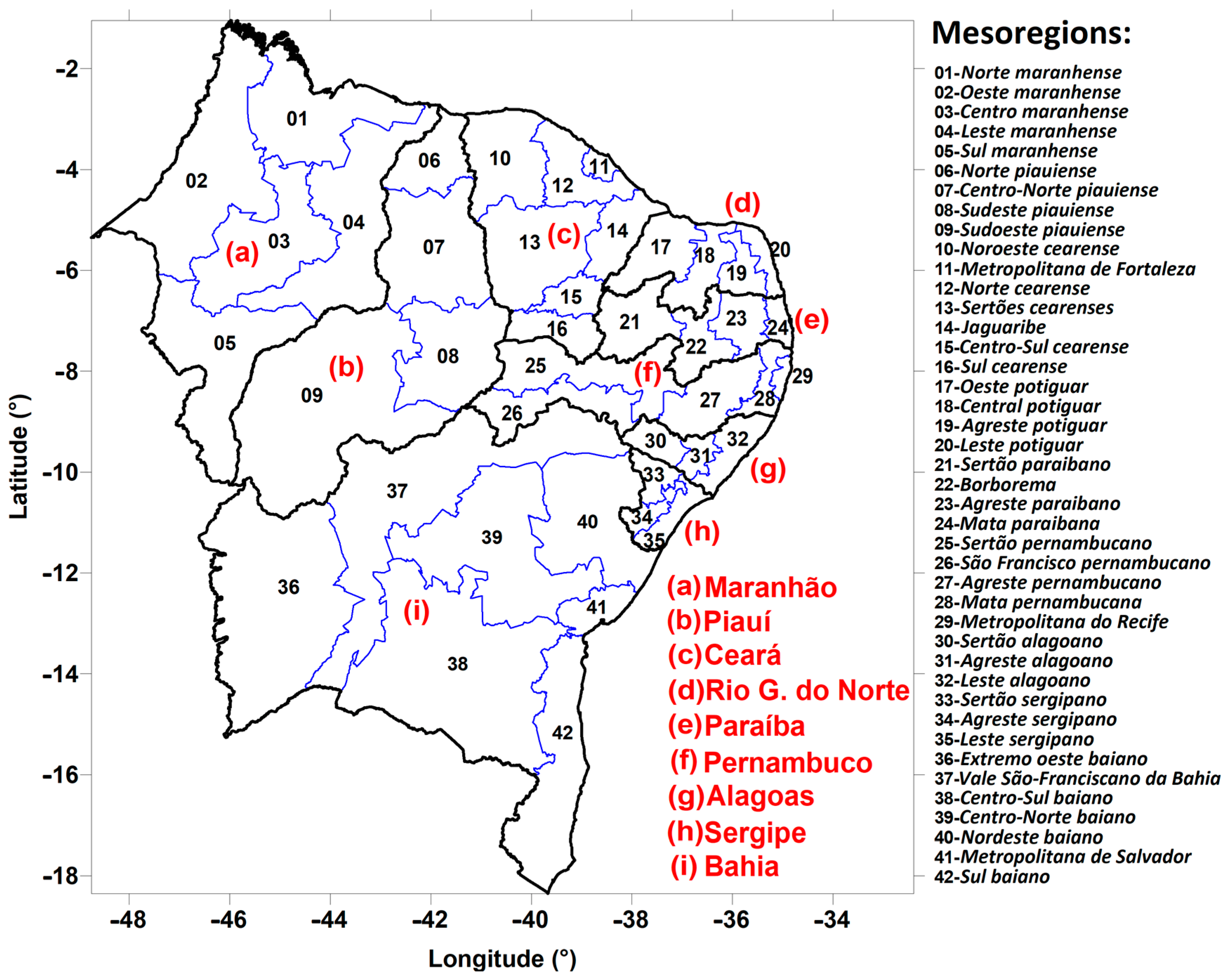
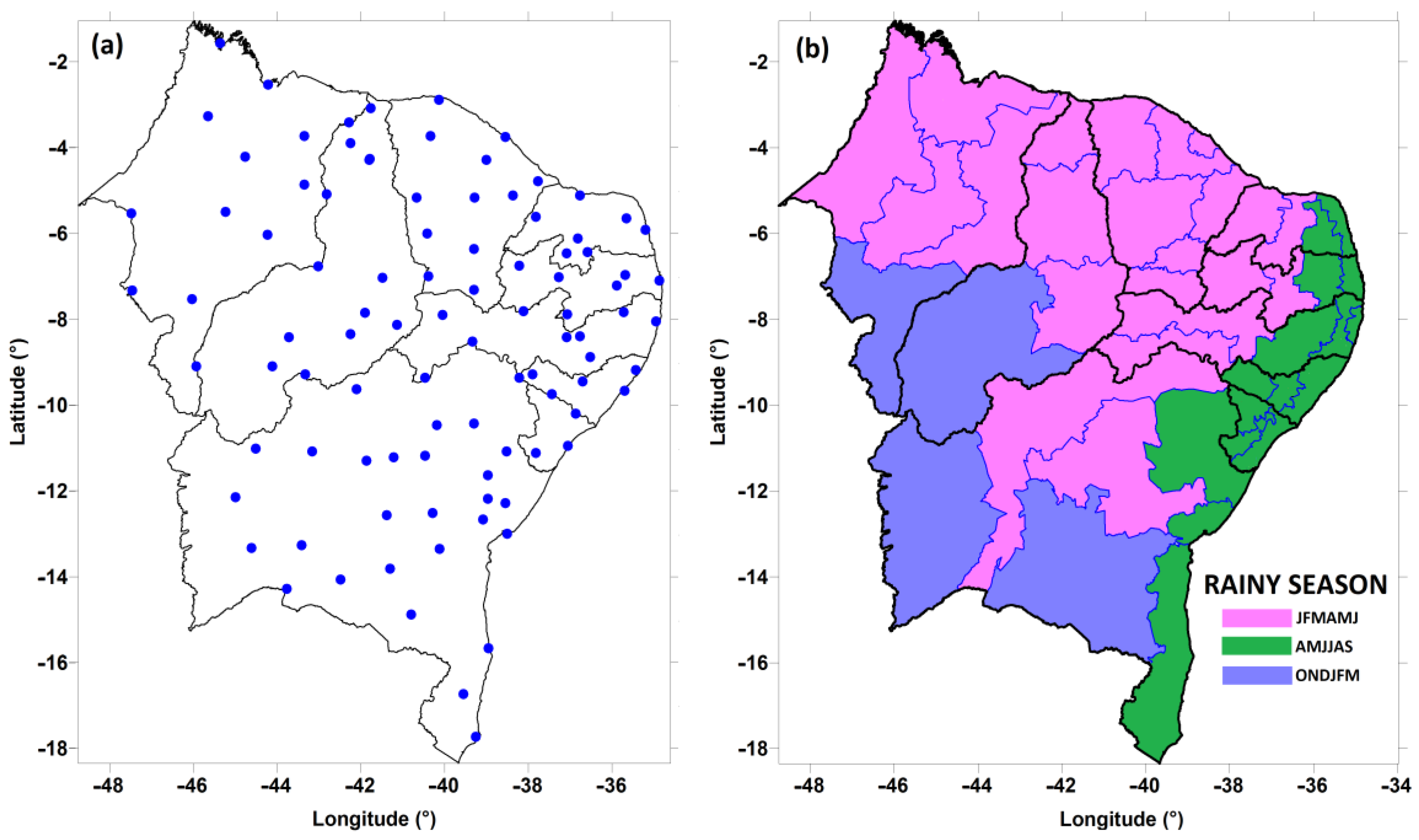
2.1. Data and Area of Study

The NEB is located between latitudes 1° and 21° S, and between longitudes 32° and 49° W, occupying around 18% of the Brazilian territory with 1.6 × 10⁶ km2 [26], divided into nine states: Maranhão (MA), Piauí (PI), Ceará (CE), Rio Grande do Norte (RN), Paraíba (PB), Pernambuco (PE), Alagoas (AL), Sergipe (SE) and Bahia (BA). These nine states are subdivided into 42 mesoregions, as shown in Figure 1. For each mesoregion, the wettest semester was identified. This task, simple but essential to the research, was carried out to simulate maize productivity in each mesoregion considering an average cycle of 120 days for the crop, so as not to risk making the mistake of not adjusting the rainy season to the planting period. As an example, for a given mesoregion where the wettest semester is January to June, the entire crop cycle, of four months on average, would fall within it. Table 1 shows the wettest semester in each mesoregion.
We used the monthly rainfall time series from 97 weather stations of the National Institute of Meteorology (INMET), from 1961 to the present, whose data underwent the quality control and gap filling described in [27]. The location of the stations can be seen in Figure 2a, while Figure 2b shows the distribution of the mesoregions by rainy semester.
The yield data were collected from the Statistical Database of the Automatic Retrieval System (SIDRA) of the Brazilian Institute of Geography and Statistics (IBGE), for the period from 1974 to 2018. However, the rainfall and yield database was worked on for a common period to eliminate continuity problems observed at the beginning of the maize yield series for each mesoregion, homogenizing them without the need to fill in gaps. The common period of data was from 1981 to 2010, 30 years, the same period used to generate the rainfall climatology for each mesoregion and identify the wettest semesters.

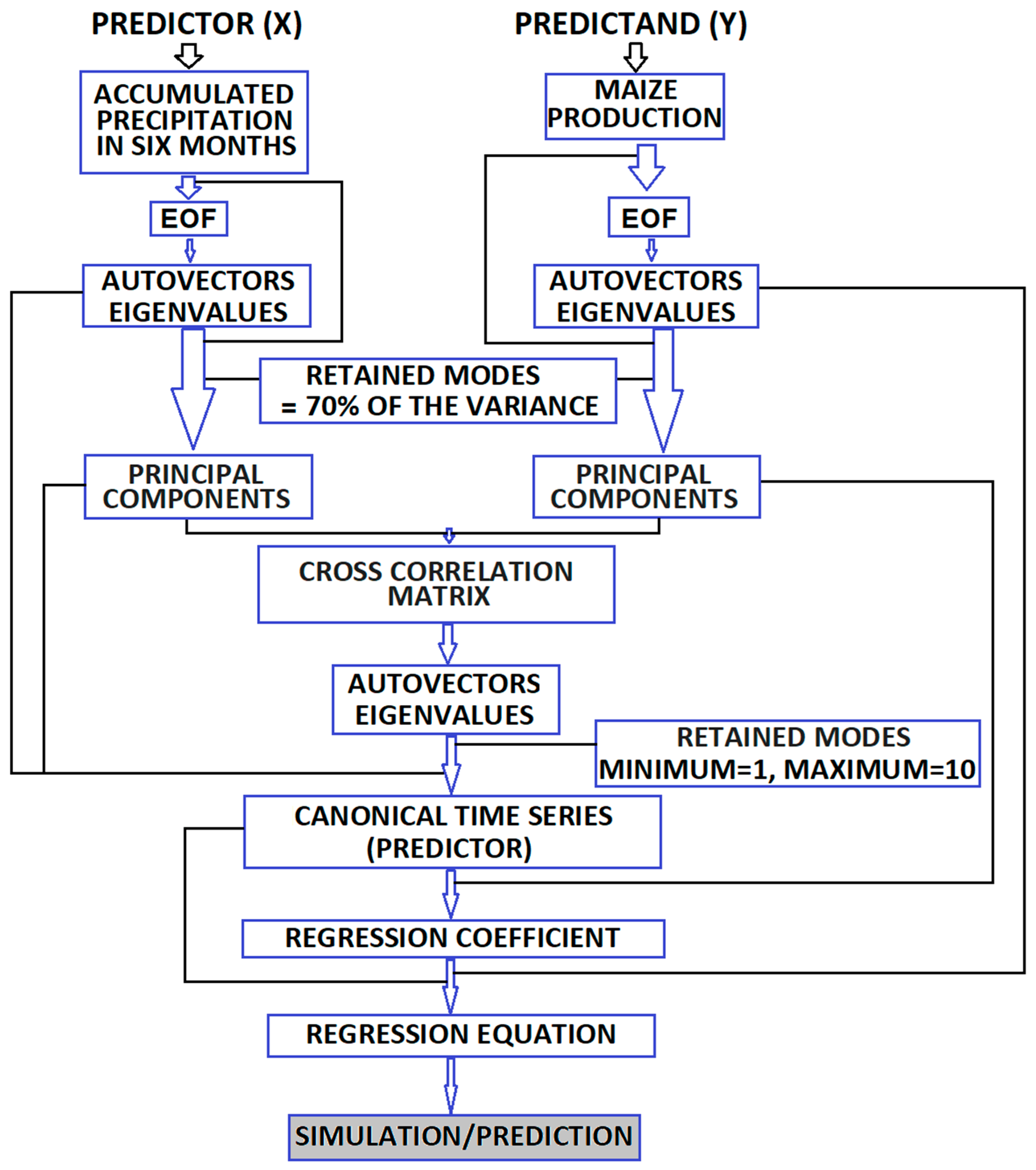
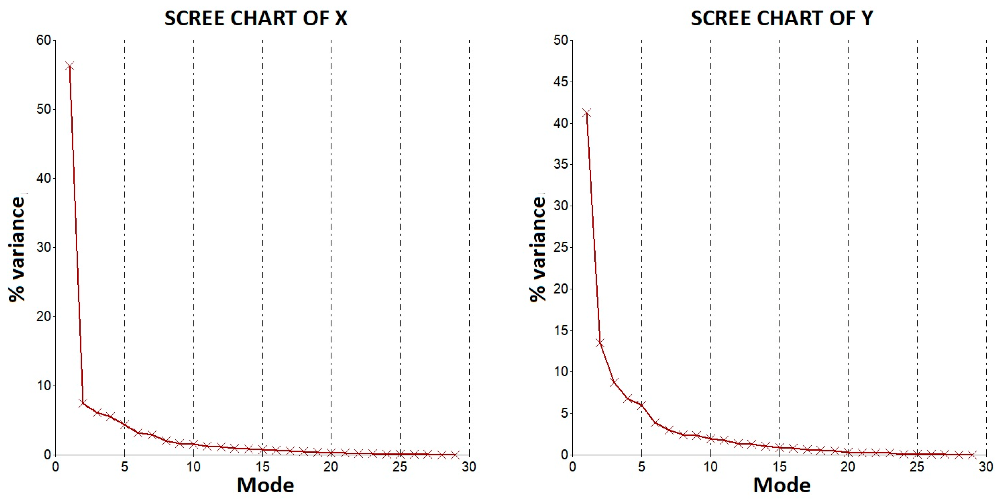
2.2. Canonical Correlation Analysis

CCA is a multivariate analysis technique widely used to generate operational climate forecasts [28,29,30]. It can be used in two ways (see Figure 1 of [31]): the first by relating raw outputs from dynamic models to observations—for example, relating predicted cumulative precipitation of a month/quarter relative to a past reference period (hindcast) with the actual observations of that period, and thus recalibrate and correct biases in these predictions, allowing this correction to be applied to future model predictions; the second way, and the method used in this research, is to build a purely statistical forecasting model, relating a predictor to a predictand; in our case, observed precipitation fields with maize production data in mesoregions of the NEB. This methodology is like seasonal forecasting with CCA, relating TSM (predictor) to precipitation (predictand).
Precipitation totals for the JFMAMJ, AMJJAS, and ONDJFM semesters were the predictors (X), and the average maize yield for each NEB mesoregion was the predictand (Y). Both fields are pre-filtered with Empirical Orthogonal Functions (EOF) to eliminate noise from the original data [32]. In this process, the EOFs of X and Y are calculated separately, establishing a model that retains around 70% to 80% of the original variance of each variable from several eigenvectors. This process forces the CCA to emphasize the dominant modes of variability of X and Y. Next, a cross-correlation matrix is constructed with the series of principal components of X and Y, whose dimensions are reduced to the number of modes retained by the predictor and the predictand, obtaining canonical eigenvectors and eigenvalues for X and Y from this transposed matrix.
The canonical function of the predictor is found from the linear combinations between the canonical eigenvectors and the series of principal components of the predictor for each mode. Although a limited number of modes can be used based on the analysis of variance explanation, it is recommended to set a minimum of 1 mode to a maximum of 10 modes as limits in the script developed in R software, version 4.0.3 (https://www.r-project.org/ (accessed on 5 August 2023)). This is recommended because it allows the software to automatically find the optimum number of modes based on a model goodness index, which adjusts the number of modes according to the correlation obtained from testing various models with different combinations of modes for X and Y, which generally limits the number of modes to between 3 and 6, respectively. The regression equation expressed by the canonical modes is derived from the original variables by converting the canonical temporal function of the predictor into the canonical temporal function of the predictand.
Finally, the predictive equation is obtained to relate the predictor to the predictand, or X to Y, and historical simulations and/or forecasts can be carried out. This research was limited to historical simulations, and it is recommended for subsequent research to test the model for forecasts based on outputs from models such as the NMME family [33] and ECMWF [34]. Figure 3 provides a schematic illustration of the steps required to simulate production (predictand Y) as a function of the six-month accumulated rainfall fields (predictor X).
To assess the relationship between accumulated rainfall and maize yield, before and after the application of CCA, we used Pearson’s correlation coefficient (r), given by Equation (1), which serves to measure the strength of the linear relationship between sets of data. We used the parametric Student’s t-test to verify the statistical significance of the correlations at a 95% confidence interval (p-value < 0.05), which according to the sample size, indicates a critical correlation coefficient of approximately 0.4, a value for which the statistical hypothesis that there is a correlation between the data sets can be accepted, in this case, between the cumulative six-month rainfall and maize production in each mesoregion of the NEB.
The other metrics used to evaluate the model were the root-mean-square error (RMSE) and the normalized root-mean-square error (NRMSE). The main advantage of the RMSE is that it penalizes errors of greater magnitude, in the same unit as the variable of interest, in our case, the production in kg/ha simulated in each mesoregion by the CCA model. Therefore, the greater the difference between simulations and observations, the greater the RMSE values [27]. However, the accuracy of the model is not well assessed with the RMSE, and it is necessary to assess it objectively. To fulfill this function, the NRMSE is a metric indicated by showing in percentage terms how much the model tends to estimate values that are closer or further away from the observation. The RMSE can be normalized by the mean of the observations, by the difference between the maximum and minimum values observed, by the standard deviation of the observation, and even by the interquartile range. In our case, we obtained the NRMSE by normalizing the RMSE with the mean of the observations, due to the high interannual variability of the observations over the 30 years analyzed. In general, NRMSE values < 20% indicate good model performance. The RMSE and NRMSE are obtained according to Equations (1) and (2) below.
R M S E ( s , o ) = 1 n i = 1 n ( s i o i ) 2
N R M S E = R M S E μ
where n is the total number of elements in the series, si = simulated value (s) by the model in each year i, oi = observed production in each year i, and µ is the average of the observations.

3. Results and Discussion

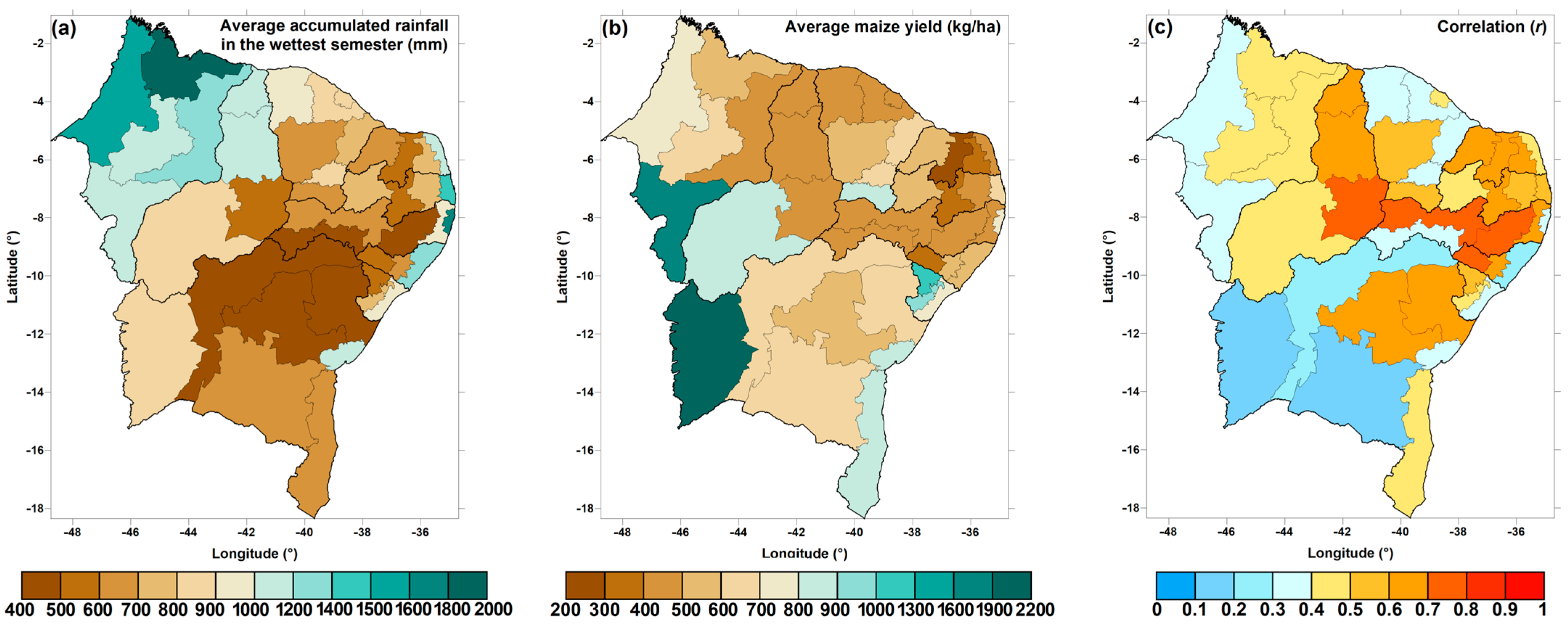
3.1. Relation between Rainfall and Production

Figure 4 shows the average accumulated rainfall in the wettest semester for each NEB mesoregion (Figure 4a), the average production for each mesoregion (Figure 4b), and the direct correlation between rainfall data and production in the 1981–2010 period (Figure 4c). Figure 4a shows that the highest accumulated rainfall is observed in all the mesoregions of the state of Maranhão, in the Norte and Centro-Norte mesoregions of Piauí, and in mesoregions of the eastern band of the NEB, between the states of Rio Grande do Norte and Bahia, with values that exceed, on average, 1000 mm of accumulated rainfall, with the maximum observed in the mesoregion Norte maranhense, at 1960 mm. In contrast, the lowest accumulated rainfall values occur in mesoregions of the central portion of the NEB, from Ceará to Bahia, with the lowest values belonging to the São Francisco and Agreste mesoregions in Pernambuco (407 mm and 458 mm), and in the Vale São-Franciscano, Centro-Norte and Nordeste mesoregions in Bahia (405 mm, 413 mm and 441 mm).
Figure 4b shows that the highest yields are concentrated in the Sul maranhense, Sudoeste piauiense and Extremo oeste baiano mesoregions (1710 kg/ha, 825 kg/ha, and 2158 kg/ha, respectively), within the region known as MATOPIBA, where cheap land prices, climate, and topography are favorable to extensive rainfed agriculture [35]. In most of the other central mesoregions of the NEB, the semi-arid climate makes them extremely vulnerable to adversities such as droughts, which are recurrent, raising the risks of loss of income for small farmers who depend on growing crops that are not well adapted to droughts, such as maize, whose production is generally less than 800 kg/ha, or less than a fifth of the average yield in other Brazilian regions [26].
The correlation (r) between accumulated rainfall in the wettest semester and observed production in the 1981–2010 period is shown in Figure 4c. Many mesoregions show r values of less than 0.4, i.e., without statistical significance according to the Student’s t-test used. However, for other mesoregions the correlation exceeds this value, showing that there is a significant relationship between accumulated rainfall in the growing season (wettest semester) and production. However, this relationship is not enough to reliably predict production values, especially in series that have some kind of trend, and it is necessary to apply some method that allows accumulated rainfall to be used as input data for predicting production.

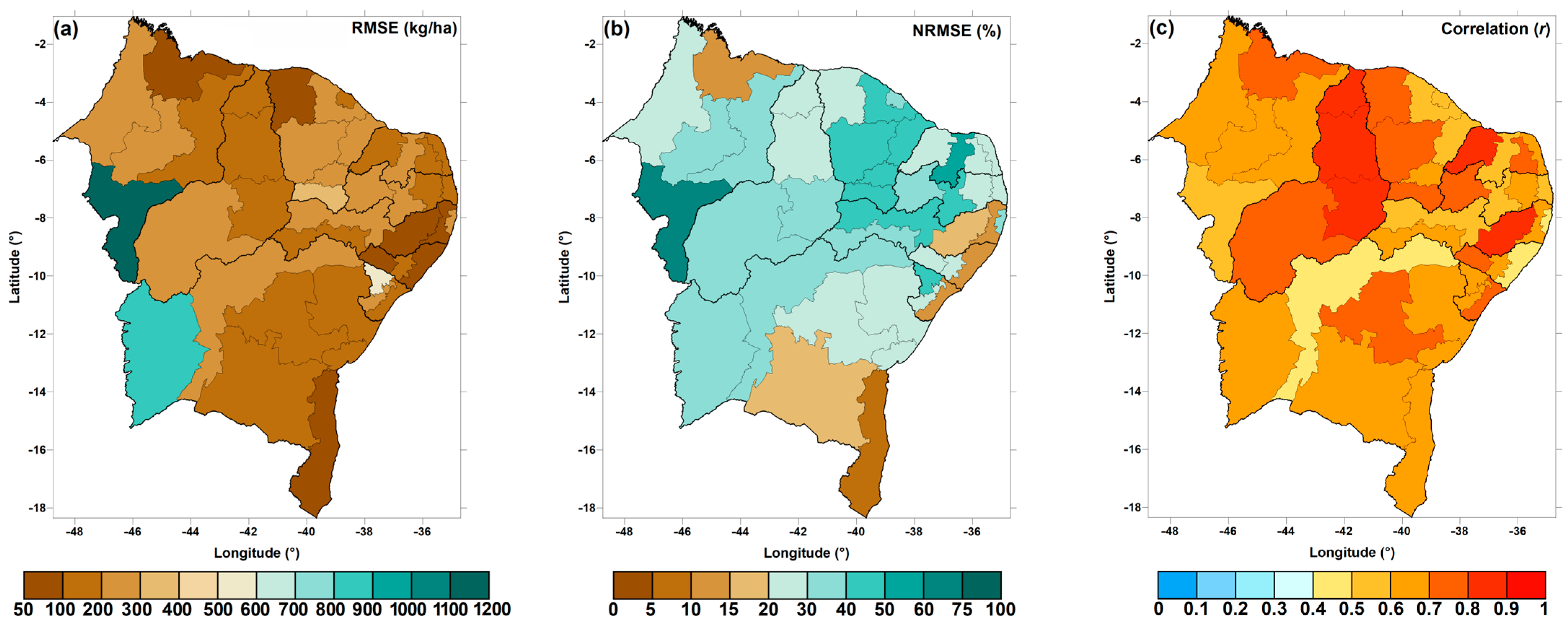
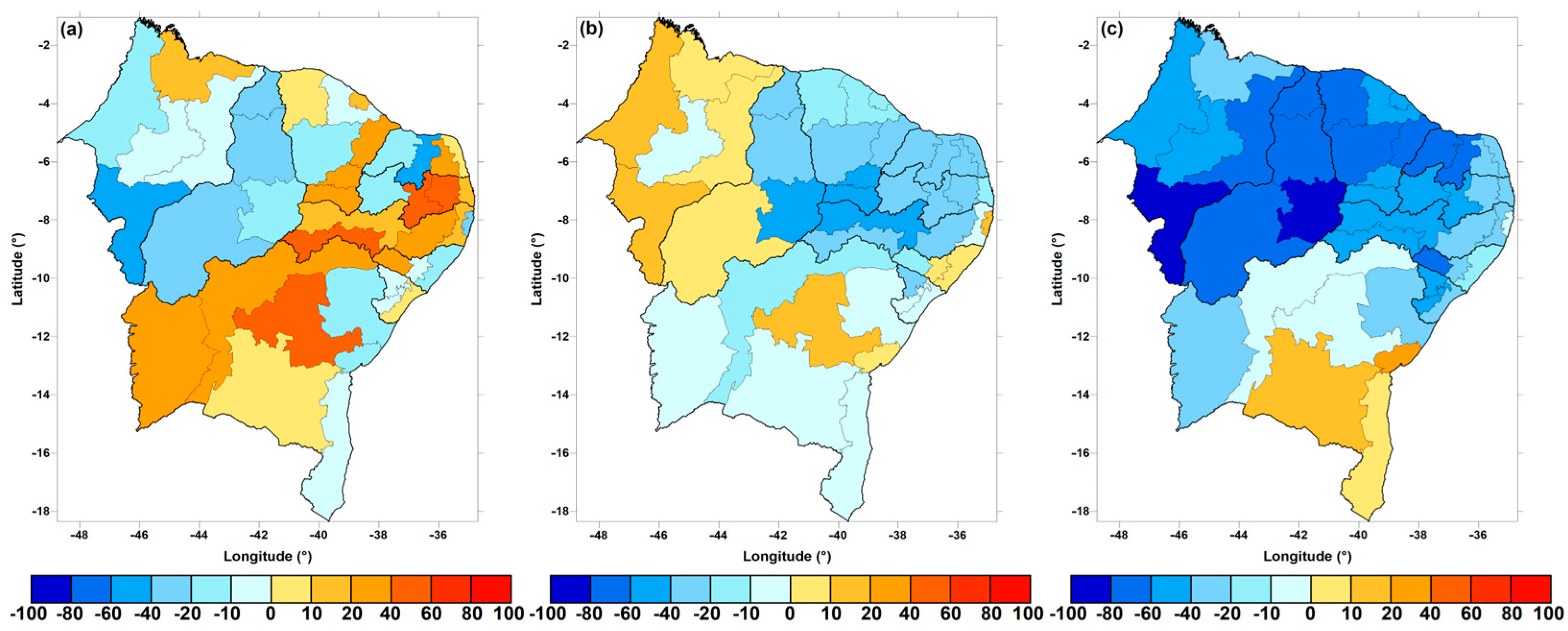
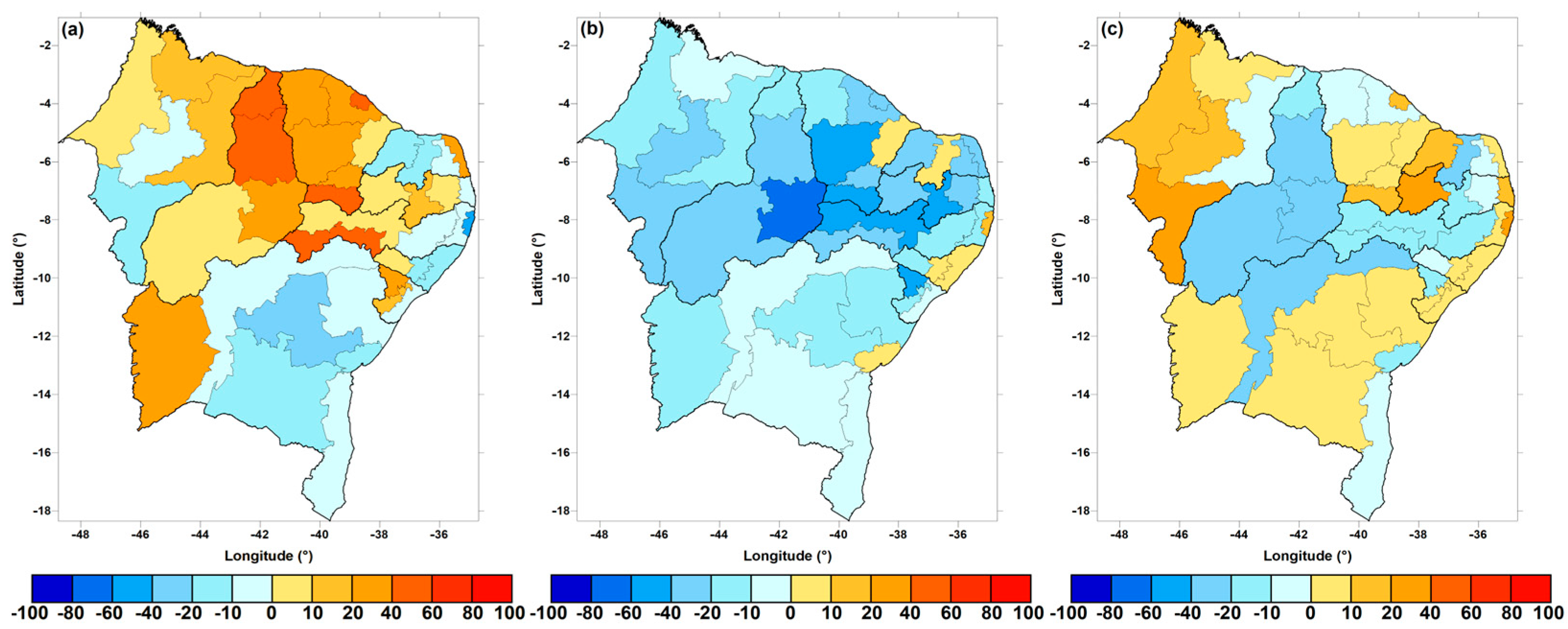
3.2. Results Obtained by the CCA Model

After checking the wettest semester in each mesoregion, shown in Figure 2, the CCA model was designed to operate with 1 to 10 modes of variability, following the flowchart shown in Figure 5. The explanatory variable, or predictor (X), was the accumulated rainfall, considering the wettest semester in each mesoregion and in which, according to the CONAB agricultural calendar, maize is grown. For each mesoregion, the variable to be explained, or predicted (Y), was obtained, which was the average production in kg/ha of the mesoregion obtained from IBGE. The model was built for 30 years from 1981 to 2010.
Figure 5 shows, for the centroid of each NEB mesoregion, the spatial loadings of the first mode of variability for predictor X and predictor Y. The first mode is the most dominant in the correlation between accumulated rainfall and production, showing that canonical loads associated with above-average rainfall are associated with above-average production. The canonical correlation for this pair of variables was 0.92 for the first mode, which explains more than 50% of the variance in the production data, directly proportional, as indicated in Figure 6. According to [36], retained modes of variability that explain more than 70% of the variance in the data are sufficient for building a predictive statistical model, since other modes can only add noise to the model without necessarily improving the predicted values.
In simpler terms, the association between the rainfall in the wettest half of the year and the production observed in each mesoregion is defined by the linear combination of the index values associated with each of the sets (EOFs), maximizing the correlation between the two indices and retaining as much information as possible contained in the original variables. Figure 5 shows scree plots for X and Y. The scree plot in multivariate statistics shows the line of factors or principal components of the analysis and is used to determine the number of factors retained or principal components maintained in an analysis, in this case, CCA. Figure 6 shows that for X, the first five factors explain 83% of the variance, and these were chosen to build the prediction model (57% for the first mode or principal component, 8% for the second mode, 7% for the third mode, 6% for the fourth mode and 5% for the fifth mode). The correspondence in Y for the first five modes is consistent with the X modes, only with percentages of explanation of the variance of the production data slightly below those observed in the X modes (accumulated rainfall).
Interpreting the RMSE as the average deviation of the forecasts from the observations, Figure 7a shows a strong predominance of deviations of less than 300 kg in most mesoregions, with seven of them having values of less than 100 kg/ha, in the Norte maranhense, Noroeste cearense, Agreste and Mata pernambucana, Sertão and Leste alagoano, and Sul baiano. The exception is the mesoregions of Sul maranhense and Extremo oeste baiano, with RMSE values of more than 800 kg/ha. This is because these mesoregions belong to the MATOPIBA area, whose agricultural activity is different from the others, being practiced extensively with a clear tendency for productivity to increase from the 2000s onwards. This upward trend in production throughout the series makes it difficult to simulate the model, which is unable to follow this behavior accurately, resulting in strong differences between the predicted and observed values, thus increasing the forecast errors, which are naturally reflected in the high RMSE values.
Taking as a reference that NRMSE values < 20% indicate good model performance, it can be seen that the model was highly accurate in the historical simulation of corn production in the mesoregions of Norte maranhense, Agreste pernambuco, Mata pernambucana, Leste alagoano, Leste sergipano, Centro-Sul baiano and Sul baiano. Moderate accuracies of between 20 and 40% were observed in 24 mesoregions in all states. NRMSE values of more than 40%, indicating low model accuracy, were observed in most of the mesoregions in the state of Ceará, with an average NRMSE of 43%, in Sertão pernambucano, Borborema and Sertão sergipano. In the Central potiguar mesoregion, the NRMSE was 52%, and the maximum value was observed in the Sul maranhense mesoregion, with NRMSE = 69%. Except for these two mesoregions with values exceeding 50%, the overall average NRMSE in all the other mesoregions was 29%, indicating a moderate prediction of the values simulated by the CCA model. It should be pointed out that a possible limiting factor in obtaining higher accuracies was the use of only one variable as a predictor of production—in this case, the cumulative six-month rainfall. Other factors are important for estimating production, such as other meteorological variables like temperature and solar radiation intensity, as well as other non-climatic factors that potentially influence production. The addition of meteorological variables other than rainfall in the construction of this model, for example, is a future objective of this research in the search for improvements in production estimates in the mesoregions of the NEB.
The map of correlations between observed and predicted production by the CCA model (Figure 7c) demonstrates its efficiency by raising all the r values obtained from the simple comparison between accumulated rainfall and production. There was an average increase of 27% in the r values. Of the 42 mesoregions among all the NEB states, in 39 the correlations between production simulated with CCA and observed, using the rainfall of the wettest semester as a predictor of production, were higher than the direct correlation between accumulated rainfall and production. The RMSE, NRMSE and r values are shown in detail in Table 2.

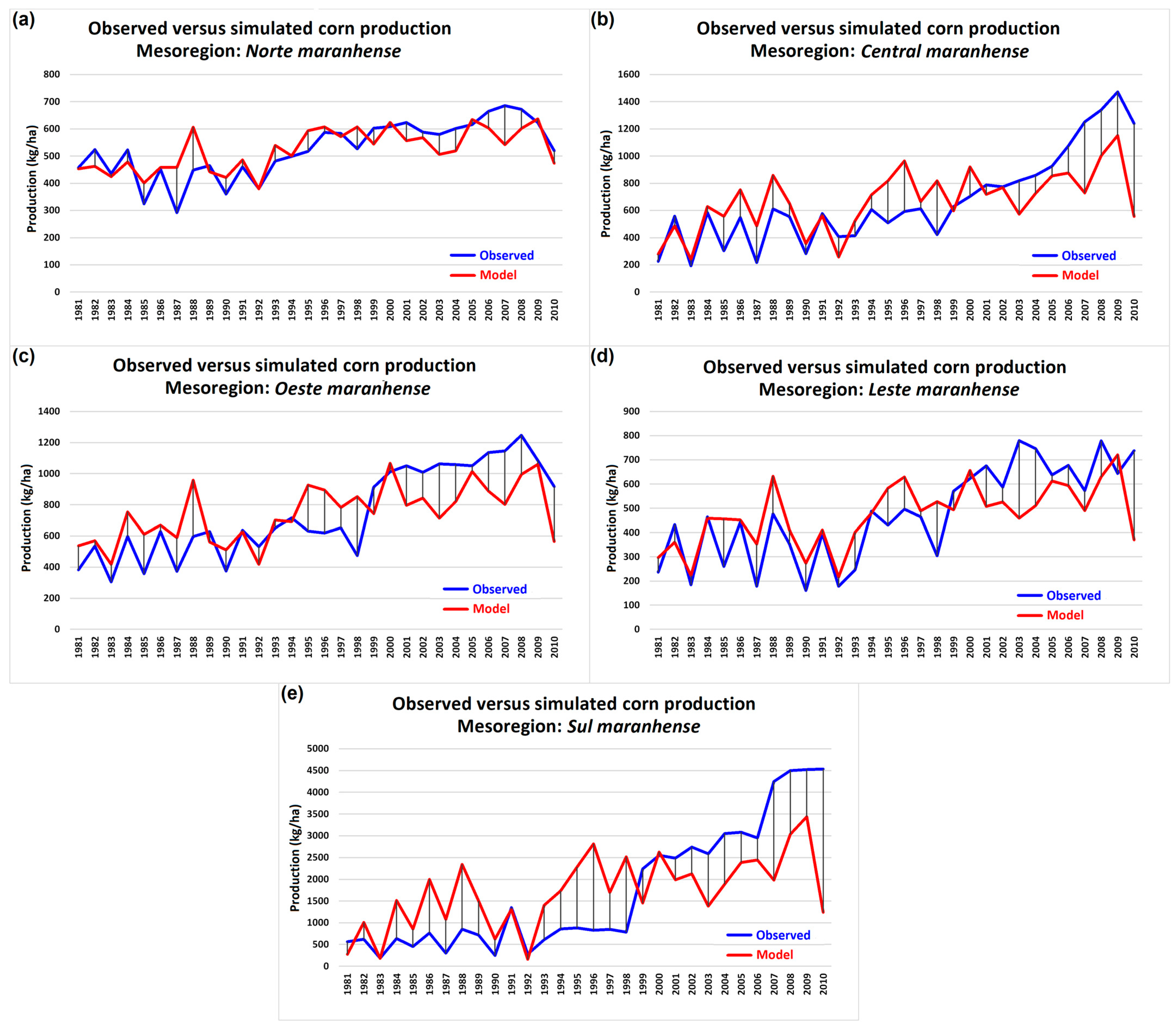
3.3. Results by State—Maranhão

The state of Maranhão has maize production in all mesoregions. In the period of analysis of this research, 1981–2010, the average produced in each mesoregion was 523 kg/ha in Norte maranhense, 746 kg/ha in Oeste maranhense, 670 kg/ha in Central maranhense, 474 kg/ha in Leste maranhense and 1710 kg/ha in Sul maranhense. The graphs in Figure 8 show the comparison between the production observed and simulated by the model in each mesoregion. There is good agreement between simulation and observation, especially in Norte maranhense (Figure 8a), with the model following the increase in observed production from 1995 onwards, although underestimating observations from 2000 onwards. This underestimation is also seen in Oeste maranhense (Figure 8b), which showed an upward trend in production from 2000 onwards. In Central maranhense, the upward trend begins in 1998 and the model underestimates from 2003 onwards (Figure 8c), with a similar situation seen in Leste maranhense (Figure 8d). Finally, this characteristic of increased production is more pronounced in Sul maranhense (Figure 8e), as a result of the advance of the agricultural frontier called MATOPIBA, which has one of its most productive areas in the south of the state [37,38]. It is important to note that, in each mesoregion, especially in the Sul maranhense, before the increase in production, the model shows a positive bias, overestimating the observed production.

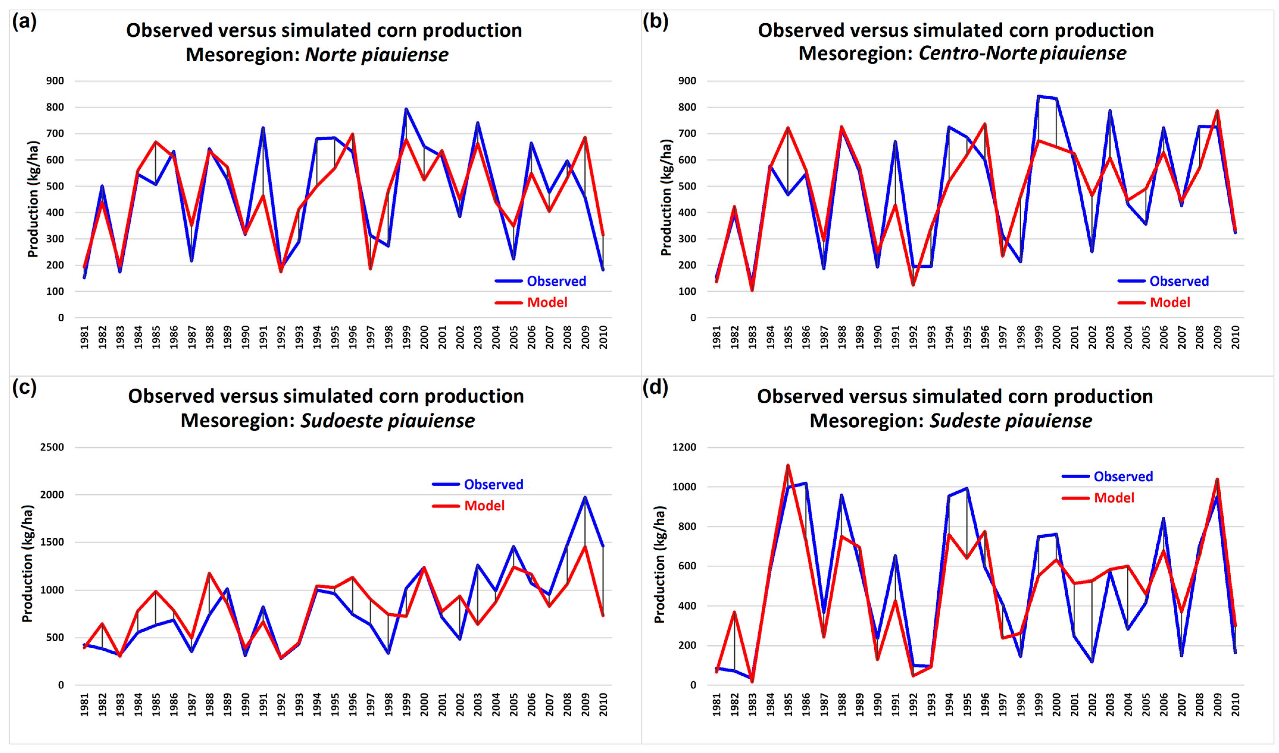
3.4. Results by State—Piauí

The results of the model simulations for Piauí showed an excellent fit with the observations. The correlation values obtained were high: 0.81 for the Norte piauíense (Figure 9a), 0.82 for the Centro-Norte piauíense (Figure 9b), 0.83 for the Sudoeste piauiense (Figure 9c) and 0.70 for the Sudeste piauiense (Figure 9d). Average production in the period is similar between the Norte piauíense, Centro-Norte piauíense, and Sudoeste piauiense mesoregions, at around 480 kg/ha. In the Sudeste piauiense, it is around 825 kg/ha, as is the case for the south of Maranhão, as a result of the MATOPIBA agricultural expansion [38], which has advanced in this mesoregion of Piauí; although soybeans are the mainstay of production [39,40], maize is also planted on a larger scale than in the other mesoregions of the state. Figure 8 shows that the model was able to simulate and capture most of the variation in production in all mesoregions. These results show that in Piauí, the response between the independent variable (accumulated rainfall) and the dependent variable (production) is more direct than in other mesoregions in other states. The rainfall regime in Piauí is associated with the southward shift of the ITCZ [41], with its interannual variations being decisive for the quality of the rainy season in the north of the NEB [42], being the main factor in the success or failure of crops. Furthermore, in the mesoregion of southwestern Piauí, rainfall events that occur from October to March [43] are equally important.

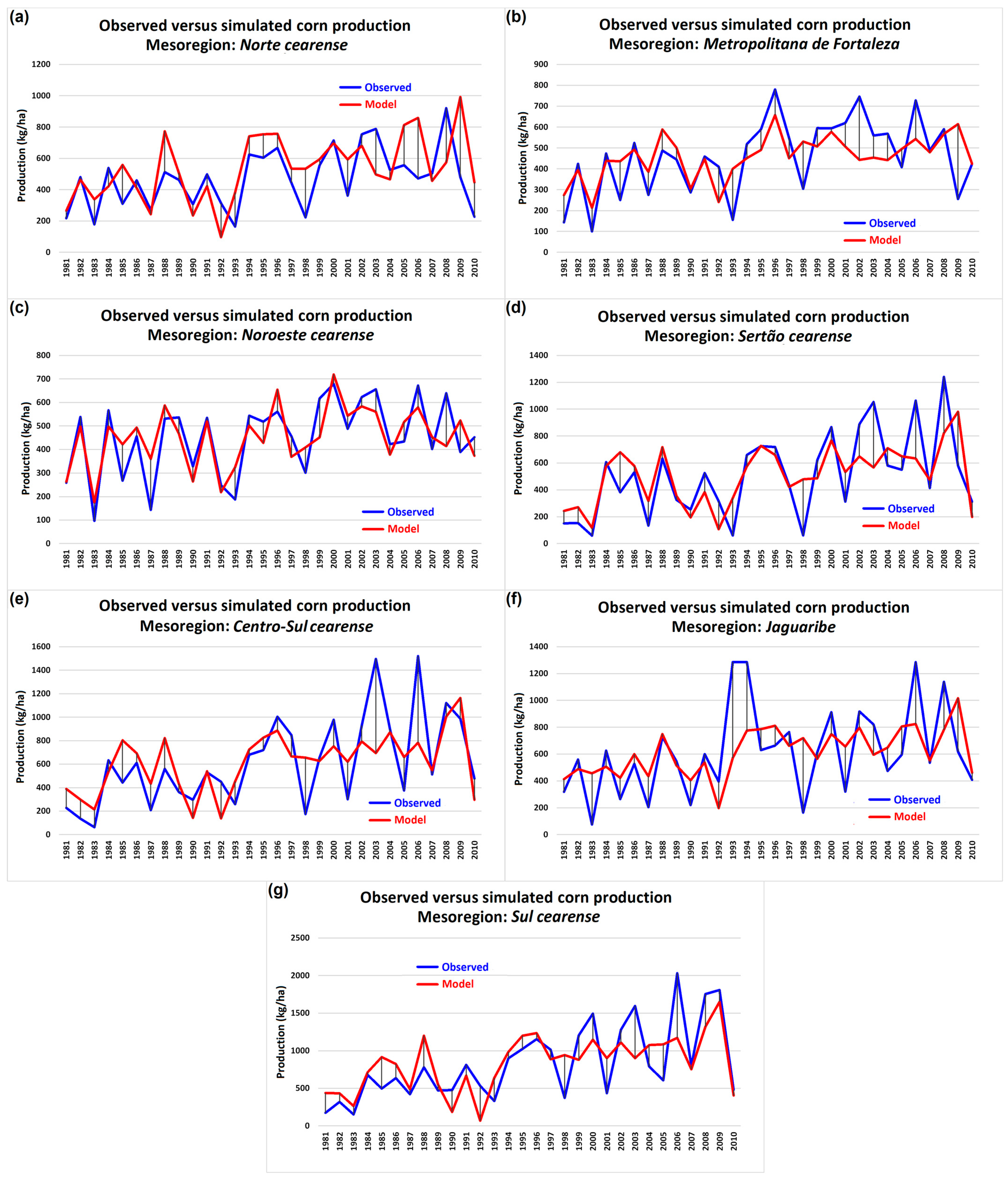
3.5. Results by State—Ceará

Ceará has seven mesoregions (Figure 10), due to the dismemberment of the municipalities bordering the capital, which formed the Metropolitana de Fortaleza mesoregion (Figure 10b). Throughout the state, the wettest period is the JFMAMJ semester, influenced by systems such as upper tropospheric cyclonic vortices (UTCV), which peak between January and February [44], ITCZ between February and April [45], remnants of easterly wave disturbances (EWD) in May and June [46], in addition to the interaction between larger-scale phenomena, such as frontal systems that induce the formation of mesoscale convective complexes [47,48]. However, as in the entire northern sector of the NEB, there is great interannual variability and poor spatial-temporal distribution of rainfall in the growing season, reflecting in years with higher and lower production.
This pattern of alternating more/less productive years (periods) was well captured by the model simulations in all mesoregions. Among these, the best performance based on correlations was seen in the Sul cearense (Figure 10g), followed by the Sertão cearense (Figure 10d), Centro-Sul cearense (Figure 10e), the Metropolitana de Fortaleza (Figure 10b), Jaguaribe (Figure 10f) and the Norte cearense (Figure 10a).

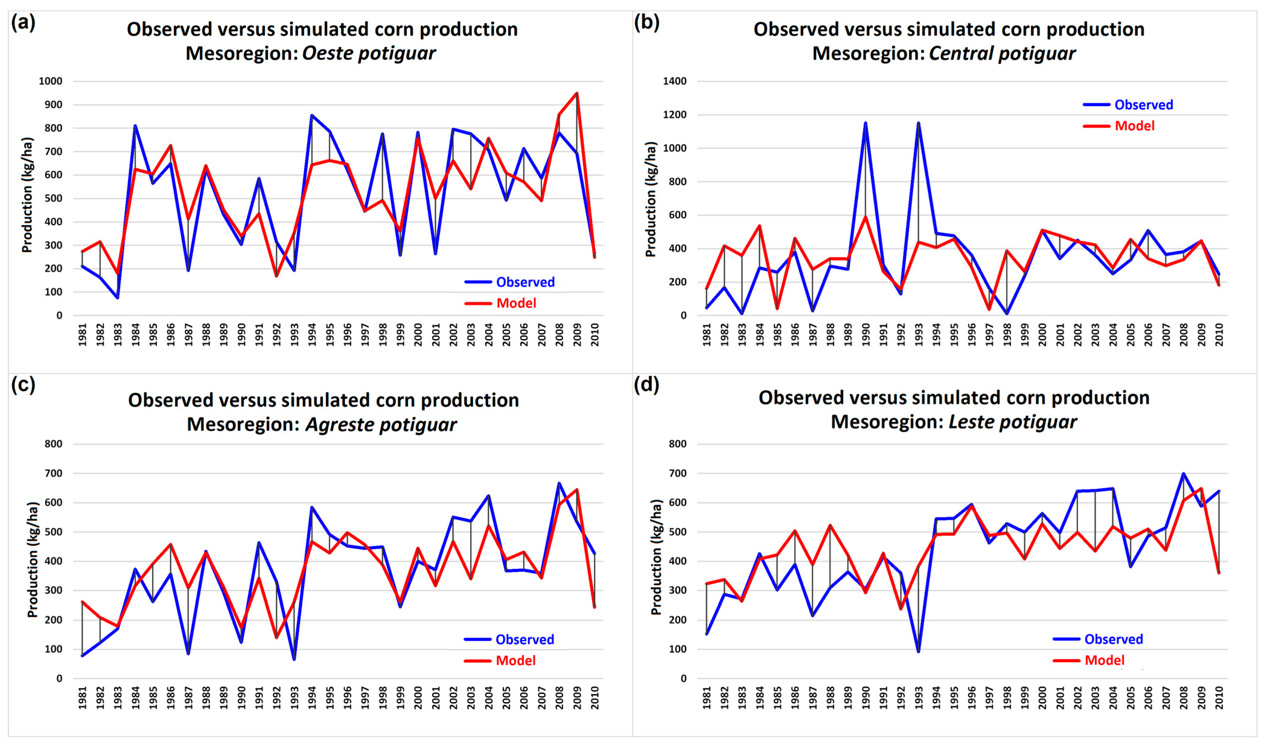
3.6. Results by State—Rio Grande do Norte

In Rio Grande do Norte, the best performance of the simulations was seen in the Oeste potiguar and Agreste potiguar mesoregions, with correlations of 0.80 and 0.74, respectively (Figure 11a and Figure 11c), following the trend of increased production from the mid-1990s onwards. The Central potiguar mesoregion (Figure 11b) showed the lowest correlation between simulations and observations, influenced by two positive peaks in the 1990 and 1993 observations not captured by the forecast model. The observed value estimated by the IBGE for 1993, in particular, is suspect due to all the other mesoregions showing low production values in that year, as can be seen most clearly in the Leste potiguar mesoregion (Figure 10d). The year 1993 was influenced by the continuation of a warm phase of ENOS (El Niño), classified as strong in the 1991–1992 biennium and weak in the 1992–1993 biennium, i.e., a sequence of three years under the influence of an extended El Niño, which on average reduces rainfall, especially in the states of the northern sector of the NEB [49].

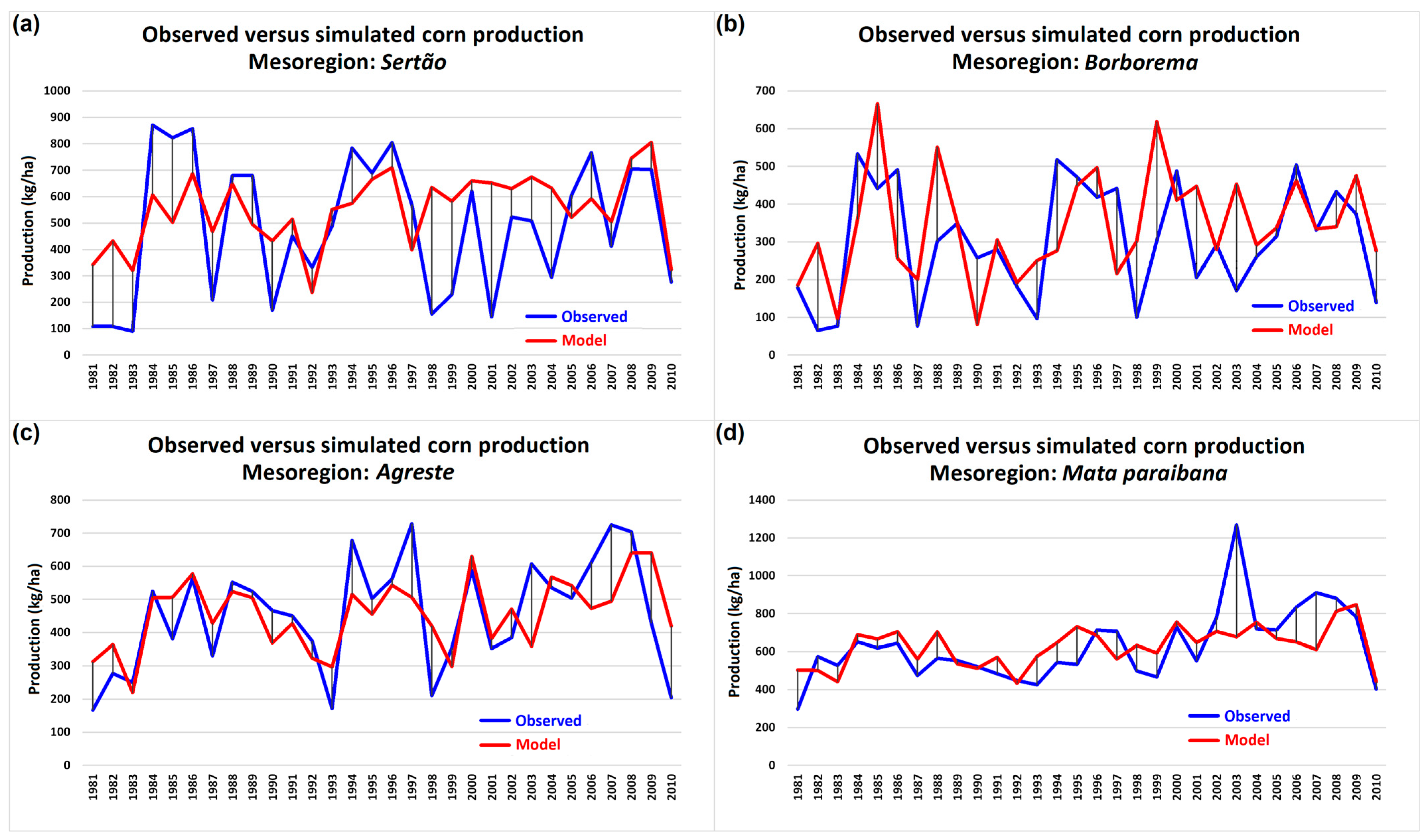
3.7. Results by State—Paraíba

As observed for Rio Grande do Norte, the western sector of Paraíba, in its Sertão paraibano mesoregion, showed the highest correlations between simulated and observed production (r = 0.71), followed by the Agreste paraibano, Mata paraibana and Borborema mesoregions, the latter of which is considered to be one of the areas with the lowest rainfall rates in Brazil [50]. The model’s ability to capture the observed behavior can be seen, although it has difficulty simulating some specific positive/negative peaks observed in the 1981–2010 period. Between 1994 and 1997, the model captured and simulated the above-average observations well, most clearly in the Sertão (Figure 12a), Borborema (Figure 12b) and Agreste (Figure 12c) mesoregions. The Mata paraibana mesoregion (Figure 12d) showed a peak in observed production in 2003 which was not captured by the model. Unlike the peak observed in 1993 in the central mesoregion of Rio Grande do Norte, this is not a suspicious value, as it was also a year of high production values observed in the Agreste mesoregion.

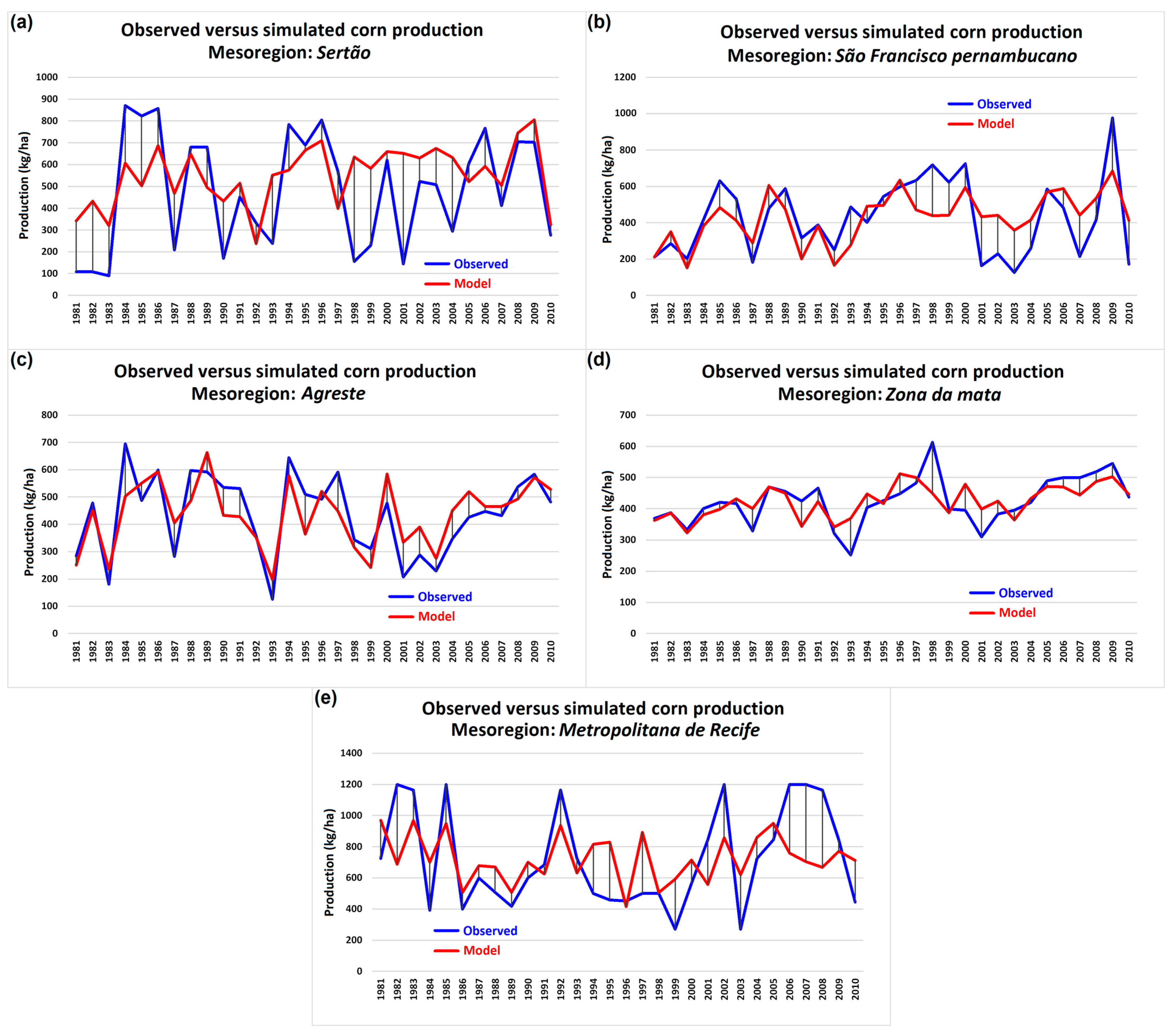
3.8. Results by State—Pernambuco

Maize production is very homogeneous in four of Pernambuco’s five mesoregions, with average values of 480 kg/ka in Pernambuco’s Sertão (Figure 13a), 428 kg/ha in the São-Francisco Pernambucano (Figure 13b), 437 kg/ha in the Agreste (Figure 13c) and 424 kg/ha in the Zona da Mata (Figure 13d), with only the Metropolitana de Recife mesoregion differing from this homogeneity with an average production of 725 kg/ha (Figure 13d).
The model simulated the observations well, without preferential bias, with the highest correlation with observations obtained for the Agreste (r = 0.81), and the lowest in the Metropolitana de Recife mesoregion (r = 0.48). The low maize yields in most of Pernambuco’s mesoregions reflect the practice of rainfed agriculture and the fact that this is one of the Northeastern states with the highest rate of return from moderate to severe droughts [25,51].

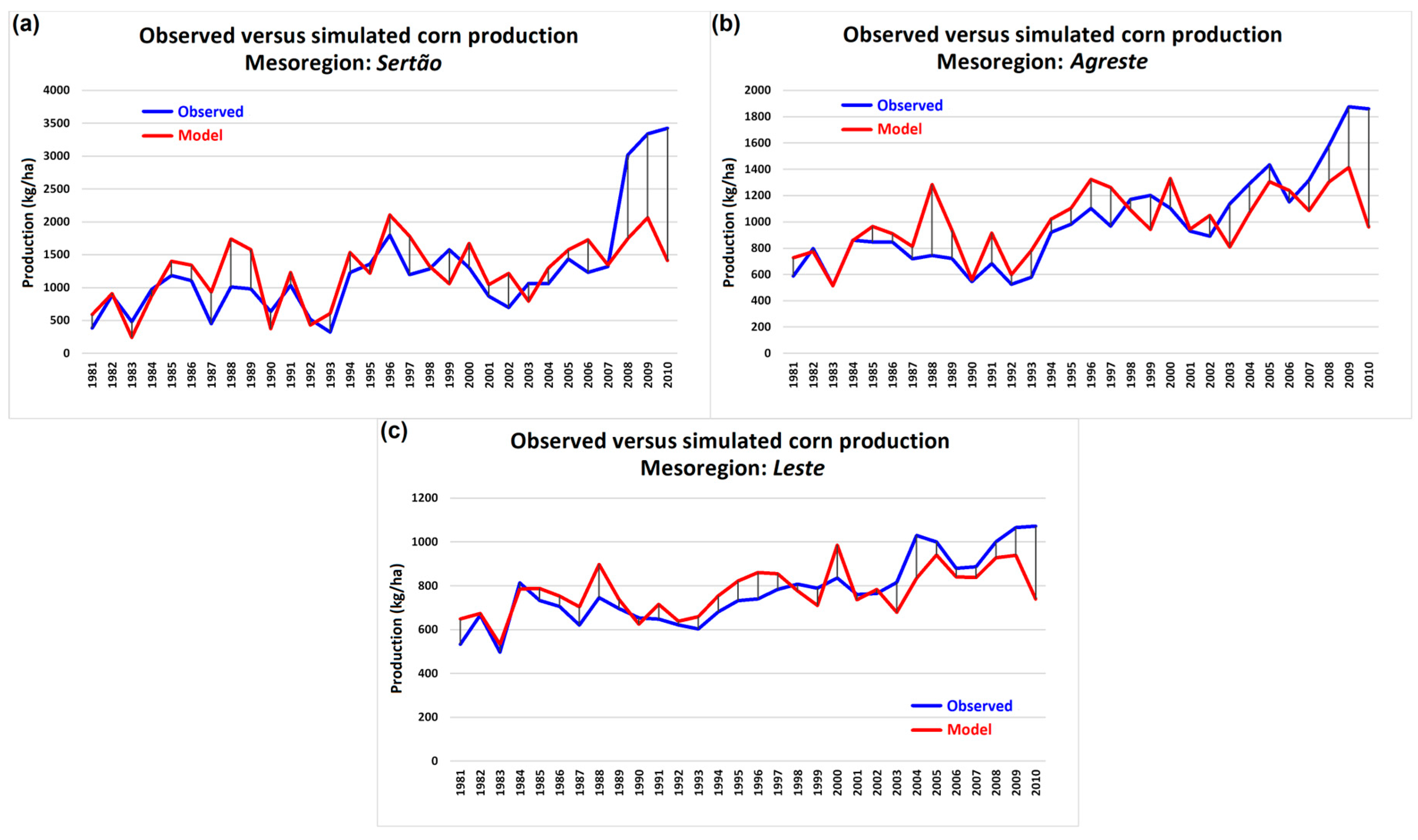
3.9. Results by State—Alagoas and Sergipe

Alagoas and Sergipe are two states in the east of the Northeast with similarities between them. Both have three mesoregions, Sertão, Agreste and Leste, and they have the same climate regime, with the wettest period, or growing season, from April to September, whose greatest influence on the precipitation regime is due to the transport of moisture from the Atlantic Ocean by the east/southeast trade winds, which are often associated with EWDs [46]. Kouadio et al. [52] evaluated extreme rainfall events in the eastern NEB and investigated their climatic causes, concluding that phenomena of different natures on different time scales are responsible for the rainfall dynamics in this region, such as ENOS, the Atlantic dipole and the Pacific decadal oscillation.
However, grain production, in this case maize, shows differences between the mesoregions of these states in the period analyzed. Alagoas has an average production of 359 kg/ha in the Sertão mesoregion (Figure 14a), 567 kg/ha in the Agreste mesoregion (Figure 14b), and 533 kg/ha in the Leste mesoregion (Figure 14c), which are lower than the values observed for Sergipe, with an average production of 1239 kg/ha in the Sertão (Figure 15a), 997 kg/ha in the Agreste (Figure 15b), and 773 kg/ha in the Leste (Figure 15c). The differences in the Leste and Agreste sectors can be explained by the greater predominance of sugar cane cultivation in these mesoregions of Alagoas than in Sergipe [53]. However, the large difference observed in production in the Sertão mesoregion of each state needs to be better investigated. In [54], da Silva et al. cite the incentives of agricultural credit and soil type as determining factors for the expansion of maize cultivation in Sergipe, and policies relating to the effect of Agricultural Climate Risk Zoning, a Brazilian agricultural policy that exerted a superior effect on maize productivity in the Sertão compared to neighboring municipalities in other mesoregions [55].
It is worth noting that the entire Agreste and Leste of these states, and the northeastern mesoregion of Bahia, have been experiencing strong growth in terms of agricultural expansion, in a new agricultural frontier called SEALBA [56], with high potential for mechanized agriculture. Such effects of grain production in SEALBA, such as maize, occurred after 2010, so this effect has not yet been detected in the analysis period of this research, 1981–2010.
The models best simulated the variability of maize production in the mesoregions of Sertão of Alagoas (r = 0.79) and Leste of Sergipe (r = 0.71). In the other mesoregions, it was efficient at following trends and some peaks in observed production.

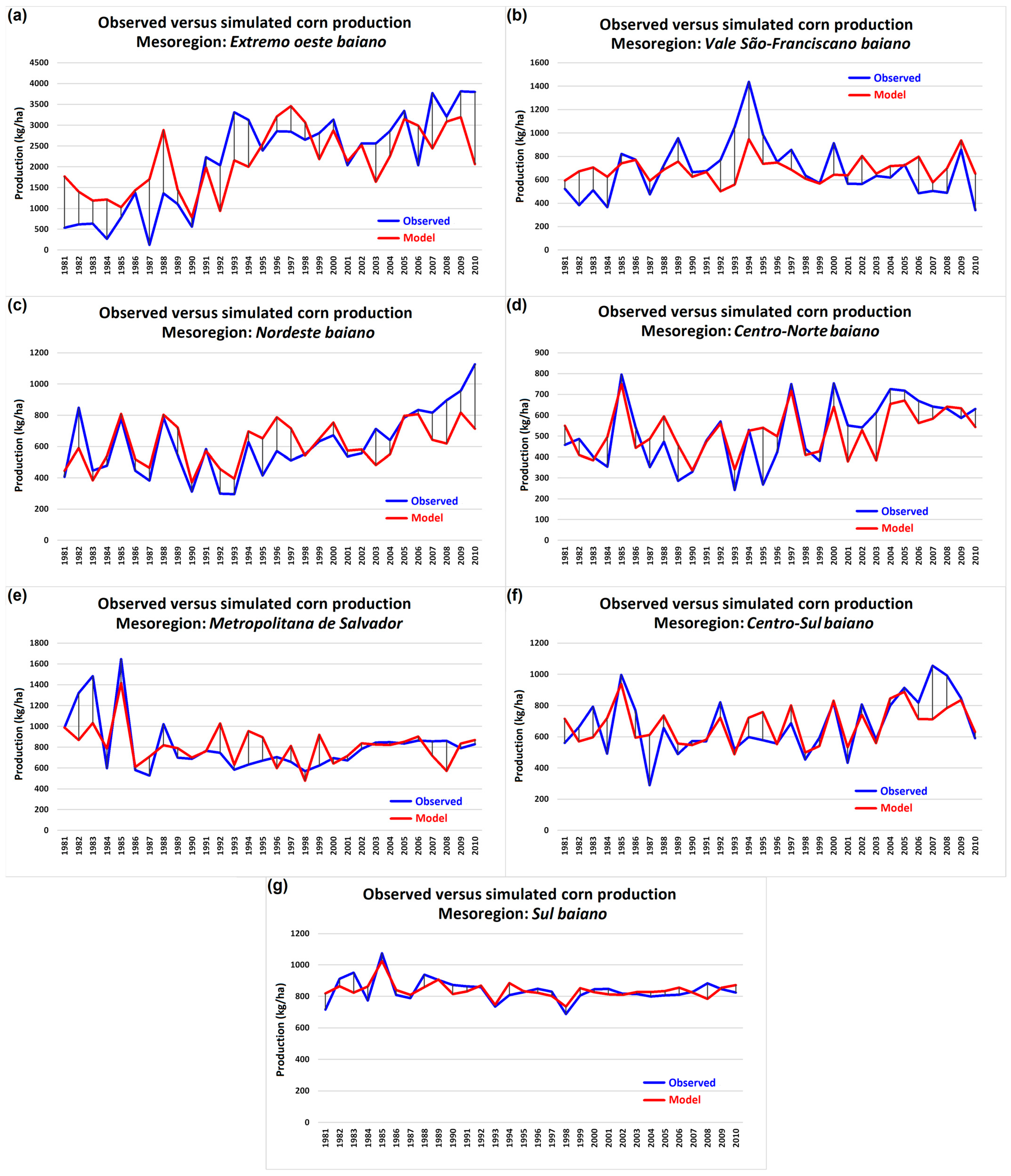
3.10. Results by State—Bahia

The largest state in the NEB, Bahia has seven mesoregions: Extremo oeste baiano, Vale são-franciscano baiano, Nordeste baiano, Centro-norte baiano, Metropolitana de Salvador, Centro-Sul baiano and Sul baiano. Average production from 1981 to 2010 ranged from 521 kg/ha in the Centro-Norte baiano to 2158 kg/ha in the Extremo oeste baiano, around 650 kg/ha in the Vale São-Franciscano baiano, the Centro-Sul baiano and the Nordeste baiano, and around 820 kg/ha in the Metropolitana de Salvador and the Sul baiano. Due to its size and different forms of cultivation, Bahia is a classic example of a state that has three distinct productivity classes: high productivity in the far west, related to the area of the state that is part of MATOPIBA [57], moderate productivity in the Sul baiano and the Metropolitana de Salvador, and low productivity in the other mesoregions.
The biggest challenge in developing any model is having it capture random peaks and trends in a time series. In this more specific case, the challenge would be for the model to capture the abrupt change in the level of productivity observed in Extremo oeste baiano from the 1990s onwards with the advance of the agricultural frontier in this sector of the state [58].
Figure 16a shows the simulation versus observation in the Extremo oeste baiano, and it is clear that the model has captured the new average production level, which jumped from an average of around 1000 kg/ha between 1981 and 1990 to an average of around 2700 kg/ha between 1991 and 2010, with a tendency to increase again towards the end of the series, with a correlation of 0.68 between simulated and observed values.
In the other mesoregions, as observed in the analyses for the other states, it can be seen that the model is capable and simulates the observed behavior well. The correlations between simulations and observations were 0.43 in the Vale São-Franciscano baiano, the lowest among the mesoregions (Figure 16b), 0.67 in the Nordeste baiano (Figure 16c), 0.72 in the Centro-Norte baiano (Figure 16d), 0.69 in the Metropolitana de Salvador (Figure 16e), 0.67 in the Centro-Sul baiano (Figure 16f), and 0.69 in the Sul baiano (Figure 16g).

3.11. Ocean-Atmosphere Interaction versus Production

Analysis of the performance of the CCA-based model showed that, in all the mesoregions of the NEB, the observed annual production of maize can be well simulated by this type of statistical modeling. It was also observed that there was a great deal of interannual variability in production, which was well captured by the model. However, the climate of the NEB is complex, and the distribution of rainfall is the response of various oceanic and atmospheric phenomena connected to each other. Classic studies have already demonstrated the relationship between the El Niño-Southern Oscillation (ENOS) and the intraseasonal and interannual variability of the ITCZ [59,60]. The dipole of sea surface temperature anomalies in the North and South Atlantic (DIP) also has a strong influence on the rainfall dynamics of the NEB [61,62]. As these phenomena in their different phases occur simultaneously, there are up to nine different combinations when relating the phases of ENOS and DIP: negative DIP + negative Pacific (La Niña), negative DIP + neutral Pacific, negative DIP + positive Pacific (El Niño), neutral DIP + negative Pacific, neutral DIP + neutral Pacific, neutral DIP + positive Pacific, positive DIP + negative Pacific, positive DIP + neutral Pacific and positive DIP + positive Pacific.
Each year between 1981 and 2010 was classified based on these combinations, as shown in Table 3. Then, the percentage deviations of the average production for each pair of combinations were obtained concerning the average production observed for each mesoregion in the 1981–2010 period. The classification of the Pacific phases was based on the Oceanic Niño Index (ONI, https://origin.cpc.ncep.noaa.gov/products/analysis_monitoring/ensostuff/ONI_v5.php (accessed on 5 August 2023)), described in [63], and of the DIP phases on the difference between SST anomalies in an area of the North Atlantic from 5.5° N to 23.5° N and from 15° W to 57.5° W, with SST anomalies in the South Atlantic from 0° to 20° S and from 10° E to 20° W (https://psl.noaa.gov/data/correlation/tna.data; https://psl.noaa.gov/data/correlation/tsa.data (accessed on 5 August 2023)) [64,65].
Figure 17 shows the average percentage yield deviations for the DipNeg/PacNeg (a), DipNeg/PacNeu (b) and DipNeg/PacPos (c) combinations. The mesoregions in the semi-arid interior between the states of Piauí, Ceará, Rio Grande do Norte, Paraíba and Pernambuco mostly showed yield gains, with the exception of the Norte, Oeste and Sul maranhense, and Extremo oeste baiano for the negative dipole and negative Pacific combination (Figure 17a), all the mesoregions of Maranhão, central-eastern Bahia, Sergipe and Alagoas (Agreste and Leste mesoregions) for the negative dipole and neutral Pacific combination (Figure 17b). The combination of years with a negative dipole and a positive Pacific was the one in which most of the mesoregions showed an average increase in production, especially the whole of the north of the NEB, Alagoas and Sergipe in the east of the NEB, and the mesoregions of western Bahia, the Vale São-Franciscano baiano, the Nordeste baiano, Metropolitana de Salvador and Sul baiano (Figure 17c), reaching more than 60% with the average in the Sertão mesoregion of Sergipe.
Under neutral DIP conditions, most of the mesoregions in the north of the NEB show positive deviations in production in relation to the average, while the opposite occurs in most of the mesoregions in the east of the NEB (Figure 18a). For the combination of neutral DIP and neutral Pacific, except for a few mesoregions which showed a low positive deviation in production, most mesoregions showed negative deviations, i.e., production below the average, of up to −60% in the Sudeste piauiense (Figure 18b). The combination of neutral DIP and positive Pacific does not show homogeneity, with mesoregions alternating positive and negative deviations, with the negative deviations more concentrated in the mesoregions of Piauí and Pernambuco, and the positive deviations in Centro-Oeste maranhense, Centro-Sul cearense, and the far east of the NEB (Figure 18c).
Finally, there is the analysis of the combinations for positive DIP and Pacific phases. For positive DIP and negative Pacific, the western portion of the NEB, which involves most of the mesoregions of Maranhão, Piauí, and some of Ceará, Rio Grande do Norte and Paraíba, showed on average a reduction in the percentage of production, a fact also observed in the mesoregions of the eastern NEB from Pernambuco to Bahia (Figure 19a). The combination of positive DIP and neutral Pacific (Figure 19b) already showed most of the central-eastern NEB with negative deviations in production, with the notable exception of mesoregions in Maranhão and the Sudoeste piauiense. The combination of positive DIP and positive Pacific represented the most damaging situation for maize production, exceeding −80% in Sul maranhense and Sudeste piauiense, with the exception of the Centro-Sul baiano, Metropolitana de Salvador and Sul baiano mesoregions (Figure 19c).
This fact has already been investigated, and the results for this last combination are in line with the results obtained by [66], when they investigated the influence of the different phases of the Pacific and Atlantic on maize and bean production in Ceará between 1952 and 2000.

4. Conclusions

The CCA-based model, relating predictor (accumulated rainfall in the wettest semester, or “growing season”) and predictand (maize production by NEB mesoregion), showed moderate to high correlations in most mesoregions, corroborating its effectiveness in capturing the behavior of the time series of observations. It was observed that there were already statistically significant correlations simply relating accumulated rainfall to production, but the CCA model presented simulations with behavior more consistent with that of the observed values, increasing the correlation when using accumulated rainfall as a predictor of observed production. The RMSE used to assess the magnitude of the model’s errors showed an average error across all mesoregions of around 200 kg/ha, with some more extreme values in specific mesoregions, such as Sul maranhense and Extremo oeste baiano. The NRMSE, used to assess the accuracy of the values simulated by the model, showed high accuracy in the simulations in six mesoregions (NRMSE < 20%) and low accuracy in two mesoregions (NRMSE > 50%), with moderate accuracy in general in the remaining mesoregions, with an average value of NRMSE = 29%.
There is a well-defined statistical relationship between the climate variability of the tropical oceans (Pacific and Atlantic) and maize production, which should be similar to that of other crops. For rainfed agriculture, as is the case with most family farming in the NEB, in general for years with the combination of a negative Atlantic dipole and a negative Pacific (La Niña), there were positive deviations in production concerning the average, which was repeated even in the combination of a negative dipole and a positive Pacific (El Niño). This shows that the TSM conditions in the Atlantic tend to have a greater impact on the NEB’s climate than those in the Pacific, possibly inhibiting the negative effects (reduced rainfall) associated with weak and/or moderate El Niño events, since studies have already shown that in exceptional cases of very strong El Niños, their influence on reducing rainfall in the NEB is greater than the influence of a negative dipole condition. For neutral Atlantic dipole conditions, the most significant results came from the combination with a negative Pacific, which resulted in positive deviations in production in the north of the NEB, and a surprising result came from the combination of a neutral dipole and neutral Pacific, with a reduction (negative percentage deviations) in production in most of the northeastern mesoregions.
Finally, analyzing the three combinations of the Pacific and the positive Atlantic dipole, the result of negative deviations in production for the positive dipole and positive Pacific (El Niño) was confirmed, with the greatest effect for the north of the NEB, with some mesoregions showing relative losses of over 90% concerning the observed average production for the period.

Author Contributions

Conceptualization, F.D.d.S.S., I.C.P. and R.L.C.; methodology, F.D.d.S.S., I.C.P. and R.L.C.; software, F.D.d.S.S., I.C.P., R.L.C., H.B.G. (Helber Barros Gomes) and D.L.H.; validation, F.D.d.S.S.; formal analysis, F.D.d.S.S., I.C.P., R.L.C., H.B.G. (Helber Barros Gomes), H.B.G. (Heliofábio Barros Gomes), J.B.C.J., R.M.d.A. and D.L.H.; data curation, F.D.d.S.S.; writing—original draft preparation, F.D.d.S.S., I.C.P. and R.L.C.; writing—review and editing, F.D.d.S.S., I.C.P., R.L.C., H.B.G. (Helber Barros Gomes), H.B.G. (Heliofábio Barros Gomes), J.B.C.J., R.M.d.A. and D.L.H.; visualization, H.B.G. (Helber Barros Gomes), H.B.G. (Heliofábio Barros Gomes), J.B.C.J., R.M.d.A. and D.L.H.; funding acquisition, D.L.H. All authors have read and agreed to the published version of the manuscript.

Funding

This research received no external funding.

Data Availability Statement

The data used in the manuscript are available by writing to the corresponding authors.

Acknowledgments

We would like to thank all the institutions that made the data used in this research available free of charge. The first author would like to thank the financial support provided by FAPEAL (Fundação de Amparo à Pesquisa de Alagoas), through Notice nº E:002/2022, Process: E:60030.0000002510/2022. The second author would like to thank CAPES, which provided financial support in the form of a scholarship.

Conflicts of Interest

The authors declare no conflicts of interest.

References

  1. CONAB—Companhia Nacional de Abastecimento. Acompanhamento da Safra Brasileira de Grãos, safra 1019/20 (Quinto levantamento). Brasília, DF, v. 7 (5), 1–112; 2020. Available online: https://www.conab.gov.br/info-agro/safras/graos/boletim-da-safra-de-graos/item/download/45055_d5c43cb0752e5b39bc31987286081f88 (accessed on 5 August 2023).
  2. CONAB—Companhia Nacional de Abastecimento. Acompanhamento da Safra Brasileira de Grãos, safra 2023/24 (Quarto levantamento). Brasília, DF, v. 11 (4), 1–111; 2024. Available online: https://www.conab.gov.br/info-agro/safras/graos/boletim-da-safra-de-graos/item/download/51274_e40f1bba791d27a4c67a29c5f29781ff (accessed on 1 February 2024).
  3. Bothast, R.J.; Schlicher, M.A. Biotechnological processes for conversion of corn into ethanol. Appl. Microbiol. Biotechnol. 2005, 67, 19–25. [Google Scholar] [CrossRef]
  4. ABIMILHO. Associação Brasileira das Indústrias de Milho. Milho. 2020. Available online: http://www.abimilho.com.br/milho/cereal (accessed on 25 November 2023).
  5. Devide, A.C.P.; Ribeiro, R.L.D.; Valle, T.L.; Almeida, D.L.; Castro, C.M.; Feltran, J.C. Produtividade de raízes de mandioca consorciada com milho e caupi em sistema orgânico. Bragantia 2009, 68, 145–153. [Google Scholar] [CrossRef]
  6. Souza, A.E.; Reis, J.G.M.; Raymundo, J.C.; Pinto, R.S. Estudo da produção do milho no Brasil. S. Am. Dev. Soc. J. 2018, 4, 182–194. [Google Scholar] [CrossRef]
  7. Garnett, E.R.; Khandekar, M.L. The impact of large-scale atmospheric circulations and anomalies on Indian monsoon droughts and floods and on world grain yields—A statistical analysis. Agric. For. Meteorol. 1992, 61, 113–128. [Google Scholar] [CrossRef]
  8. Silva, B.K.d.N.; Costa, R.L.; Silva, F.D.d.S.; Vanderlei, M.H.G.d.S.; da Silva, H.J.F.; Júnior, J.B.C.; Costa Júnior, D.S.d.; Pedra, G.U.; Pérez-Marin, A.M.; Silva, C.M.S.e. Proposal of an Agricultural Vulnerability Stochastic Model for the Rural Population of the Northeastern Region of Brazil. Climate 2023, 11, 211. [Google Scholar] [CrossRef]
  9. Cavalcante, E.S.; Lacerda, C.F.; Costa, R.N.T.; Gheyi, H.R.; Pinho, L.L.; Bezerra, F.M.S.; Oliveira, A.C.; Canjá, J.F. Supplemental irrigation using brackish water on maize in tropical semi-arid regions of Brazil: Yield and economic analysis. Sci. Agric. 2021, 78, e20200151. [Google Scholar] [CrossRef]
  10. Cruz, J.C.; Pereira Filho, I.A.; Alvarenga, R.C.; Gontijo Neto, M.M.; Viana, J.H.M.; de Oliveira, M.F.; Matrangolo, W.J.R.; de Albuquerque Filho, M.R. EMBRAPA Milho e Sorgo: Cultivo do Milho, Sistemas de Produção, v. 2 (6). 2010. Available online: https://ainfo.cnptia.embrapa.br/digital/bitstream/item/27037/1/Plantio.pdf (accessed on 5 January 2024).
  11. Coelho, D.T.; Dale, R.F. An energy-crop growth variable and temperature function for predicting corn growth and development: Planting to silking. Agron. J. 1980, 72, 503–510. [Google Scholar] [CrossRef]
  12. Bonhomme, R. Bases and limits to using “degree-day” units. Eur. J. Agron. 2000, 13, 1–10. [Google Scholar] [CrossRef]
  13. Guiscem, J.M.; Sans, L.M.A.; Nakagawa, J.; Cruz, J.C.; Pereira Filho, I.A.; Mateus, G.P. Crescimento e desenvolvimento da cultura do milho (Zea mays L.) em semeadura tardia e sua relação com graus-dia e radiação solar global. Rev. Bras. Agrometeorol. 2001, 9, 215–260. [Google Scholar]
  14. Streck, N.A.; Lago, I.; Gabriel, L.F.; Samboranha, F.K. Simulating maize phenology as a function of air temperature with a linear and a nonlinear model. Pesqui. Agropecuária Bras. 2008, 43, 449–455. [Google Scholar] [CrossRef]
  15. Lacerda, F.F.; Nobre, P.; Sobral, M.C.; Lopes, G.M.B.; Chou, S.C.; Assad, E.D.; Brito, E. Long-term temperature and rainfall trends over northeast Brazil and Cape Verde. Earth Sci. Clim. Chang. 2015, 6, 296. [Google Scholar]
  16. Oliveira, P.T.; Santos e Silva, C.M.; Lima, K.C. Climatology and trend analysis of extreme precipitation in subregions of Northeast Brazil. Theor. Appl. Climatol. 2016, 130, 77–90. [Google Scholar] [CrossRef]
  17. Martins, M.A.; Tomasella, J.; Rodriguez, D.A.; Alvalá, R.C.; Giarolla, A.; Garofolo, L.L.; Júnior, J.L.S.; Paolicchi, L.T.; Pinto, G.L. Improving drought management in the Brazilian semiarid through crop forecasting. Agric. Syst. 2018, 160, 21–30. [Google Scholar] [CrossRef]
  18. Martins, M.A.; Tomasella, J.; Dias, C.G. Maize yield under a changing climate in the Brazilian Northeast: Impacts and adaptation. Agric. Water Manag. 2019, 216, 339–350. [Google Scholar] [CrossRef]
  19. Marengo, J.A.; Torres, R.R.; Alves, L.M. Drought in Northeast Brazil-past, present, and future. Theor. Appl. Climatol. 2016, 129, 1189–1200. [Google Scholar] [CrossRef]
  20. Cunha, A.P.M.A.; Alvalá, R.C.S.; Nobre, C.A.; Carvalho, M.A. Monitoring vegetative drought dynamics in the Brazilian semiarid Region. Agric. For. Meteorol. 2015, 214, 494–505. [Google Scholar] [CrossRef]
  21. Cunha, A.P.M.A.; Tomasella, J.; Ribeiro-Neto, G.G.; Brown, M.; Garcia, S.R.; Brito, S.B.; Carvalho, M.A. Changes in the spatial-temporal patterns of droughts in the Brazilian Northeast. Atmos. Sci. Lett. 2018, 19, e855. [Google Scholar] [CrossRef]
  22. Cunha, A.P.M.A.; Zeri, M.; Leal, K.D.; Costa, L.; Cuartas, L.A.; Marengo, J.A.; Tomasella, J.; Vieira, R.M.; Barbosa, A.A.; Cunningham, C.; et al. Extreme Drought Events over Brazil from 2011 to 2019. Atmosphere 2019, 10, 642. [Google Scholar] [CrossRef]
  23. Alvala, R.C.S.; Cunha, A.P.M.A.; Brito, S.S.B.; Seluchi, M.E.; Marengo, J.A.; Moraes, O.L.L.; Carvalho, M.A. Drought monitoring in the Brazilian Semiarid region. An. Acad. Bras. Ciências 2017, 91, e20170209. [Google Scholar] [CrossRef]
  24. Medeiros, F.J.; Oliveira, C.P.; Avila-Diaz, A. Evaluation of extreme precipitation climate indices and their projected changes for Brazil: From CMIP3 to CMIP6. Weather Clim. Extrem. 2022, 38, 100511. [Google Scholar] [CrossRef]
  25. Pontes Filho, J.D.; Souza Filho, F.d.A.; Martins, E.S.P.R.; Studart, T.M.d.C. Copula-Based Multivariate Frequency Analysis of the 2012–2018 Drought in Northeast Brazil. Water 2020, 12, 834. [Google Scholar] [CrossRef]
  26. Marengo, J.A.; Galdos, M.V.; Challinor, A.; Cunha, A.P.; Marin, F.R.; Vianna, M.S.; Alvala, R.C.S.; Alves, L.M.; Moraes, O.L.; Bender, F. Drought in Northeast Brazil: A review of agricultural andpolicy adaptation options for food security. Clim. Resil. Sustain. 2021, 1, e17. [Google Scholar] [CrossRef]
  27. Costa, R.L.; Barros Gomes, H.; Cavalcante Pinto, D.D.; da Rocha Júnior, R.L.; dos Santos Silva, F.D.; Barros Gomes, H.; Lemos da Silva, M.C.; Luís Herdies, D. Gap Filling and Quality Control Applied to Meteorological Variables Measured in the Northeast Region of Brazil. Atmosphere 2021, 12, 1278. [Google Scholar] [CrossRef]
  28. Mason, S.J.; Tippett, M.K. (Eds.) Climate Predictability Tool Version 15.5.10; Columbia University Academic Commons: New York, NY, USA, 2017. [Google Scholar]
  29. Esquivel, A.; Llanos-Herrera, L.; Agudelo, D.; Prager, S.D.; Fernandes, K.; Rojas, A.; Valencia, J.J.; Ramirez-Villegas, J. Predictability of seasonal precipitation across major crop growing areas in Colombia. Clim. Serv. 2018, 12, 36–47. [Google Scholar] [CrossRef]
  30. Hossain, M.Z.; Azad, M.A.K.; Karmakar, S.; Mondal, M.N.I.; Das, M.; Rahman, M.M.; Haque, M.A. Assessment of Better Prediction of Seasonal Rainfall by Climate Predictability Tool Using Global Sea Surface Temperature in Bangladesh. Asian J. Adv. Res. Rep. 2019, 4, 1–13. [Google Scholar] [CrossRef]
  31. Barnston, A.G.; Tippett, M.K. Do Statistical Pattern Corrections Improve Seasonal Climate Predictions in the North American Multimodel Ensemble Models? J. Clim. 2017, 30, 8335–8355. [Google Scholar] [CrossRef]
  32. Horel, J.D. A Rotated Principal Component Analysis of the Interannual Variability of the Northern Hemisphere 500 mb Height Field. Mon. Weather Rev. 1981, 109, 2080–2092. [Google Scholar] [CrossRef]
  33. Kirtman, B.P.; Min, D.; Infanti, J.M.; Kinter, J.L.; Paolino, D.A.; Zhang, Q.; Van Den Dool, H.; Saha, S.; Mendez, M.P.; Becker, E.; et al. The North American multimodel ensemble: Phase-1 seasonal-to-interannual prediction; phase-2 toward developing intraseasonal prediction. Bull. Am. Meteorol. Soc. 2014, 95, 585–601. [Google Scholar] [CrossRef]
  34. Wang, Q.J.; Shao, Y.; Song, Y.; Schepen, A.; Robertson, D.E.; Ryu, D.; Pappenberger, F. An evaluation of ECMWF SEAS5 seasonal climate forecasts for Australia using a new forecast calibration algorithm. Environ. Model. Softw. 2019, 122, 104550. [Google Scholar] [CrossRef]
  35. Araújo, M.L.S.; Sano, E.E.; Bolfe, E.L.; Santos, J.R.N.; dos Santos, J.S.; Silva, F.B. Spatiotemporal dynamics of soybean crop inthe Matopiba region, Brazil (1990–2015). Land Use Policy 2019, 80, 57–67. [Google Scholar] [CrossRef]
  36. Lima, C.H.R.; Kwon, H.-H.; Kim, H.J. Sparse Canonical Correlation Analysis Postprocessing Algorithms for GCM Daily Rainfall Forecasts. J. Hydrometeorol. 2022, 23, 1705–1718. [Google Scholar] [CrossRef]
  37. Salvador, M.A.; Brito, J.I.B. Trend of annual temperature and frequency of extreme events in the MATOPIBA region of Brazil. Theor. Appl. Climatol. 2018, 133, 253–261. [Google Scholar] [CrossRef]
  38. dos Reis, L.C.; Silva, C.M.S.; Bezerra, B.G.; Mutti, P.R.; Spyrides, M.H.C.; da Silva, P.E. Analysis of Climate Extreme Indices in the MATOPIBA Region, Brazil. Pure Appl. Geophys. 2020, 177, 1. [Google Scholar] [CrossRef]
  39. Assad, E.D.; Marin, F.R.; Pinto, H.S.; Zullo Júnior, J. Mudanças climáticas e agricultura: Uma abordagem agroclimatológica. Ciência Ambiente 2007, 34, 169–182. [Google Scholar]
  40. Pereira, C.N.; Castro, C.N.D.; Porcionato, G.L. Expansão da agricultura no MATOPIBA e impactos na infraestrutura regional. Rev. Econ. Agrícola 2018, 65, 15–33. [Google Scholar] [CrossRef]
  41. Utida, G.; Cruz, F.W.; Etourneau, J.; Bouloubassi, J.; Schefuß, E.; Vuille, M.; Novello, V.F.; Prado, L.F.; Sifeddine, A.; Klein, V.; et al. Tropical South Atlantic influence on Northeastern Brazil precipitation and ITCZ displacement during the past 2300 years. Sci. Rep. 2019, 9, 1698. [Google Scholar] [CrossRef] [PubMed]
  42. Marengo, J.A.; Alves, L.M.; Alvala, R.C.C.; Cunha, A.P.M.A.; Brito, S.B.; Moraes, O.L.L. Climatic characteristics of the 2010–2016 drought in the semiarid Northeast Brazil region. An. Acad. Bras. Ciências 2018, 90, 1973–1985. [Google Scholar] [CrossRef]
  43. Pezzi, L.P.; Quadro, M.F.L.; Souza, E.B.; Miller, A.J.; Rao, V.B.; Rosa, E.B.; Santini, M.F.; Bender, A.; Souza, R.B.; Cabrera, M.J.; et al. Oceanic SACZ produces an abnormally wet 2021/2022 rainy season in South America. Sci. Rep. 2023, 13, 1455. [Google Scholar] [CrossRef] [PubMed]
  44. de Morais, M.D.C.; Gan, M.A.G.; Yoshida, M.C. Features of the upper tropospheric cyclonic vortices of Northeast Brazil in life cycle stages. Int. J. Climatol. 2021, 41, E39–E58. [Google Scholar] [CrossRef]
  45. Carvalho, M.A.V.; Oyama, M.D. Variabilidade da largura e intensidade da Zona de Convergência Intertropical Atlântica: Aspectos observacionais. Rev. Bras. Meteorol. 2013, 28, 305–316. [Google Scholar] [CrossRef]
  46. Gomes, H.B.; Ambrizzi, T.; Da Silva, B.F.P.; Hodges, K.; Dias, P.L.S.; Herdies, D.; Silva, M.C.L.; Gomes, H.B. Climatology of easterly wave disturbances over the tropical South Atlantic. Clim. Dyn. 2019, 53, 1393–1411. [Google Scholar] [CrossRef]
  47. Veber, M.E.; Fedorova, N.; Levit, V. Desenvolvimento de Atividades Convectivas Sobre a Região Nordeste do Brasil, Organizada Pela Extremidade Frontal. Rev. Bras. Meteorol. 2020, 35, 995–1003. [Google Scholar] [CrossRef]
  48. Lyra, M.J.A.; Fedorova, N.; Levit, V. Mesoscale convective complexes over northeastern Brazil. J. S. Am. Earth Sci. 2022, 118, 103911. [Google Scholar] [CrossRef]
  49. Gonzalez, R.A.; Andreoli, R.V.; Candido, L.A.; Kayano, M.T.; Souza, R.A.F. A influência do evento El Niño—Oscilação Sul e Atlântico Equatorial na precipitação sobre as regiões norte e nordeste da América do Sul. Acta Amaz. 2013, 43, 469–480. [Google Scholar]
  50. Alves, J.M.; Repelli, C.A. A variabilidade pluviométrica no setor norte do nordeste e os eventos El Nino-Oscilação Sul (ENOS). Rev. Bras. Meteorol. 1992, 7, 583–592. [Google Scholar]
  51. Martins, E.S.P.R.; Coelho, C.A.S.; Haarsma, R.; Otto, F.E.L.; King, A.D.; Van Oldenborgh, G.J.; Kew, S.; Philip, S.; Júnior, F.C.V.; Cullen, H. A multimethod attribution analysis of the prolonged northeast Brazil hydrometeorological drought (2012–16). Bull. Am. Meteorol. Soc. 2018, 99, 65–69. [Google Scholar] [CrossRef]
  52. Kouadio, Y.K.; Servain, J.; Machado, L.A.T.; Lentini, C.A.D. Heavy Rainfall Episodes in the Eastern Northeast Brazil Linked to Large-Scale Ocean-Atmosphere Conditions in the Tropical Atlantic. Adv. Meteorol. 2012, 2012, 369567. [Google Scholar] [CrossRef]
  53. Marin, F.; Nassif, D.S.P. Mudanças climáticas e a cana-de-açúcar no Brasil: Fisiologia, conjuntura e cenário futuro. Rev. Bras. Eng. Agrícola E Ambient. 2013, 17, 232–239. [Google Scholar] [CrossRef]
  54. da Silva, D.S.; de Moura, F.R.; Santos e Silva, M.A.; da Silva, A.A.G. Spatial Effect Assessment on Maize Production in the Sergipe’s Backwoods. Braz. J. Dev. 2019, 5, 20677–20701. [Google Scholar]
  55. Barros, G.V.P.; Gomes, H.B.; Nascimento, P.S.R.; Pinto, D.D.C.; Silva, F.D.S.; Costa, R.L. Comparative Analysis of Potential Soil Degradation in the State of Sergipe. GEO UERJ 2023, 42, e65942. [Google Scholar]
  56. Silva, E.H.d.L.; Silva, F.D.d.S.; Junior, R.S.d.S.; Pinto, D.D.C.; Costa, R.L.; Gomes, H.B.; Júnior, J.B.C.; de Freitas, I.G.F.; Herdies, D.L. Performance Assessment of Different Precipitation Databases (Gridded Analyses and Reanalyses) for the New Brazilian Agricultural Frontier: SEALBA. Water 2022, 14, 1473. [Google Scholar] [CrossRef]
  57. Santiago, D.B.; Barbosa, H.A.; Correia Filho, W.L.F.; Oliveira-Júnior, J.F. Interactions of Environmental Variables and Water Use Efficiency in the Matopiba Region via Multivariate Analysis. Sustainability 2022, 14, 8758. [Google Scholar] [CrossRef]
  58. Matsunaga, W.K.; Sales, E.S.G.; Assis Júnior, G.C.; Silva, M.T.; Lacerda, F.F.; de Paiva Lima, E.; dos Santos, C.A.C.; de Brito, J.I.B. Application of ERA5-Land reanalysis data in zoning of climate risk for corn in the state of Bahia-Brazil. Theor. Appl. Climatol. 2024, 155, 945–963. [Google Scholar] [CrossRef]
  59. Philander, S.G.H.; Gu, D.; Halpern, D.; Lambert, G.; Lau, N.C.; Li, T.; Pacanowski, R.C. Why the ITCZ is mostly North of the Equator. J. Clim. 1996, 9, 2958–2972. [Google Scholar] [CrossRef]
  60. Trenberth, K.E. The Definition of El Niño. Bull. Am. Meteorol. Soc. 1997, 78, 2771–2777. [Google Scholar] [CrossRef]
  61. Moura, A.D.; Shukla, J. On the dynamics of droughts in northeast Brazil: Observations, theory and numerical experiments with a general circulation model. J. Atmos. Sci. 1981, 38, 2653–2675. [Google Scholar] [CrossRef]
  62. Nobre, P.; Shukla, J. Variations of Sea Surface Temperature, Wind Stress, and Rainfall over the Tropical Atlantic and South American. J. Clim. 1996, 9, 2464–2479. [Google Scholar] [CrossRef]
  63. Huang, B.; Thorne, P.T.; Banzon, V.F.; Boyer, T.; Chepurin, G.; Lawrimore, J.H.; Menne, M.J.; Smith, T.M.; Vose, R.S.; Zhang, H.-M. Extended Reconstructed Sea Surface Temperature, Version 5 (ERSSTv5): Upgrades, Validations, and Intercomparisons. J. Clim. 2017, 30, 8179–8205. [Google Scholar] [CrossRef]
  64. Enfield, D.B.; Alfaro, E.J. The Dependence of Caribbean Rainfall on the Interaction of the Tropical Atlantic and Pacific Oceans. J. Clim. 1999, 12, 2093–2103. [Google Scholar] [CrossRef]
  65. Servain, J.; Clauzet, G.; Wainer, I.C. Modes of tropical Atlantic climate variability observed by PIRATA. Geophys. Res. Lett. 2003, 30, 8003. [Google Scholar] [CrossRef]
  66. Alves, J.M.B.; Servain, J.; Campos, J.N.B. Relationship between ocean climatic variability and rain-fed agriculture in northeast Brazil. Clim. Res. 2009, 38, 225–236. [Google Scholar] [CrossRef]
Figure 1. Map of the Northeast region of Brazil identifying the nine states, (a) Maranhão, (b) Piauí, (c) Ceará, (d) Rio Grande do Norte, (e) Paraíba, (f) Pernambuco, (g) Alagoas, (h) Sergipe and (i) Bahia, and identifying the 42 mesoregions, numbered between the states.
Agriengineering 06 00051 g001
Figure 2. (a) Geographical distribution of the 97 conventional weather stations in the NEB states; (b) rainy semester for each NEB mesoregion.
Agriengineering 06 00051 g002
Figure 3. Illustrative diagram of the steps used to simulate maize production in the NEB mesoregions based on semi-annual accumulated precipitation, using CCA.
Agriengineering 06 00051 g003
Figure 4. (a) Average rainfall for the wettest semester in each NEB mesoregion, in millimeters, (b) average maize production in kg/ha, and (c) correlation between accumulated rainfall in the growing season in each mesoregion and observed production. For the sample size of 30 years, all correlations above 0.4 are statistically significant according to the Student’s t-test. Obtained for the period 1981–2010.
Agriengineering 06 00051 g004
Figure 5. Spatial loads of X and Y (mode 1) show the most dominant pattern in the correlation of rainfall associated with above-normal production. The canonical correlation for this pair of variables was over 0.92. From the time points (mode 1), rainfall patterns, above or below normal, tend to coincide with above-normal production and vice versa. They were obtained for the period 1981–2010.
Agriengineering 06 00051 g005
Figure 6. Scree plot of the number of modes retained in the principal component analysis.
Agriengineering 06 00051 g006
Figure 7. (a) RMSE in kg/ha between observed and simulated production, (b) NRMSE in % between observed and simulated production, and (c) correlation between observed and simulated production with CCA. For the sample size of 30 years, all correlations above 0.4 are statistically significant according to the Student’s t-test. Obtained for the period 1981–2010.
Agriengineering 06 00051 g007
Figure 8. Production observed (blue line) and simulated with the CCA model (red line), for the period 1981–2010, for the mesoregions of Maranhão: (a) Norte maranhense, (b) Oeste maranhense, (c) Central maranhense, (d) Leste maranhense and (e) Sul maranhense.
Agriengineering 06 00051 g008
Figure 9. The same as Figure 8, but for the mesoregions of Piauí: (a) Norte piauiense, (b) Centro-Norte piauiense, (c) Sudoeste piauiense and (d) Sudeste piauiense.
Agriengineering 06 00051 g009
Figure 10. The same as in Figure 8, but for the mesoregions of Ceará: (a) Norte cearense (b) Metropolitana de Fortaleza, (c) Noroeste cearense, (d) Sertão cearense, (e) Centro-Sul cearense, (f) Jaguaribe and (g) Sul cearense.
Agriengineering 06 00051 g010
Figure 11. The same as in Figure 8, but for the mesoregions of Rio Grande do Norte: (a) Oeste potiguar (b) Central potiguar, (c) Agreste potiguar, and (d) Leste potiguar.
Agriengineering 06 00051 g011
Figure 12. The same as in Figure 8, but for the mesoregions of Paraíba: (a) Sertão, (b) Borborema, (c) Agreste and (d) Mata paraibana.
Agriengineering 06 00051 g012
Figure 13. The same as in Figure 8, but for the mesoregions of Pernambuco: (a) Sertão, (b) São Francisco pernambucano, (c) Agreste, (d) Zona da Mata and (e) Metropolitana de Recife.
Agriengineering 06 00051 g013
Figure 14. The same as in Figure 8, but for the mesoregions of Alagoas: (a) Sertão, (b) Agreste, and (c) Leste.
Agriengineering 06 00051 g014
Figure 15. The same as in Figure 8, but for the mesoregions of Sergipe: (a) Sertão, (b) Agreste, and (c) Leste.
Agriengineering 06 00051 g015
Figure 16. The same as in Figure 8, but for the mesoregions of Bahia: (a) Extremo oeste baiano, (b) Vale São-Franciscano baiano, (c) Nordeste baiano, (d) Centro-Norte baiano, (e) Metropolitana de Salvador, (f) Centro-Sul baiano and (g) Sul baiano.
Agriengineering 06 00051 g016
Figure 17. Average deviation of production from the 1981–2010 average for years classified under the influence of the negative Atlantic dipole and (a) negative Pacific, (b) neutral Pacific and (c) positive Pacific.
Agriengineering 06 00051 g017
Figure 18. Average deviation of production from the 1981–2010 average for years classified under the influence of the neutral Atlantic dipole and (a) negative Pacific, (b) neutral Pacific and (c) positive Pacific.
Agriengineering 06 00051 g018
Figure 19. Average deviation of production from the 1981–2010 average for years classified under the influence of a positive Atlantic dipole and (a) negative Pacific, (b) neutral Pacific and (c) positive Pacific.
Agriengineering 06 00051 g019
Table 1. Mesoregions of the NEB and respective rainy semester.
MesoregionRainy Season
Norte maranhense
Oeste maranhense
Central maranhense
Leste maranhense
Norte piauiense
Centro Norte piauiense
Sudeste piauiense
Noroeste cearense
Metropolitana de Fortaleza
Norte cearense
Sertões cearensesJanuary to June
Jaguaribe(JFMAMJ)
Centro-Sul cearense
Sul cearense
Oeste potiguar
Central potiguar
Sertão paraibano
Borborema
Sertão pernambucano
São-Francisco pernambucano
Vale São Franciscano da Bahia
Centro-Norte baiano
Sul maranhense
Sudoeste piauienseOctober to March
Extremo oeste baiano(ONDJFM)
Centro-Sul baiano
Agreste potiguar
Leste potiguar
Agreste paraibano
Mata paraibana
Agreste pernambucano
Mata pernambucana
Metropolitana do Recife
Sertão alagoanoApril to September
Agreste alagoano(AMJJAS)
Leste alagoano
Sertão sergipano
Agreste sergipano
Leste sergipano
Sul baiano
Nordeste baiano
Metropolitana de Salvador
Table 2. For each mesoregion, correlation values (r) were obtained from the direct comparison of accumulated rainfall × observed production, and the production simulated by the CCA model and observed. Values in bold highlight the highest r obtained.
Mesoregionr—Accumulated Rainfall × Productionr—CCA Model × ProductionRMSE (kg/ha)NRMSE (%)
Norte maranhense0.450.746813
Oeste maranhense0.380.6521128
Central maranhense0.470.6624737
Leste maranhense0.440.6614330
Sul maranhense0.370.56117569
Norte piauiense0.620.8111524
Centro Norte piauiense0.660.8212927
Sudeste piauiense0.710.8318838
Sudoeste piauiense0.450.729736
Noroeste cearense0.330.789922
Norte cearense0.310.5120243
Metropolitana de Fortaleza0.440.5913930
Sertões cearenses0.50.721843
Jaguaribe0.370.5327444
Centro-Sul cearense0.350.6627845
Sul cearense0.50.7334341
Oeste potiguar0.690.814127
Central potiguar0.640.5215352
Agreste potiguar0.630.7421039
Leste potiguar0.420.6215149
Sertão paraibano0.430.7623148
Borborema0.60.5415637
Agreste paraibano0.630.6520830
Mata paraibana0.50.5610520
Sertão pernambucano0.760.5383239
São-Francisco pernambucano0.390.6513420
Agreste pernambucano0.750.8110930
Mata pernambucana0.640.6912227
Metropolitana do Recife0.350.4812327
Sertão alagoano0.770.7915625
Agreste alagoano0.620.638620
Leste alagoano0.20.425413
Sertão sergipano0.530.6327638
Agreste sergipano0.430.6759148
Leste sergipano0.340.7126627
Extremo oeste Baiano0.170.6810313
Vale São Franciscano da Bahia0.280.438925
Centro-Sul baiano0.160.6712422
Centro-Norte baiano0.650.727013
Nordeste baiano0.620.67526
Metropolitana de Salvador0.360.6815024
Sul baiano0.420.6918823
Table 3. Composite years are classified according to the definitions of the climatic events observed in the Pacific and Atlantic oceans. DIP: Atlantic dipole; Pac: Pacific; Neg: negative; Neu: neutral; Pos: positive.
Climate CombinationsYears
DipNeg/PacNeg1984, 1985, 1986, 1989, 2000, 2008
DipNeg/PacNeu1991, 1994
DipNeg/PacPos1988, 1995, 2003, 2009, 2010
DipNeu/PacNeg1996, 1999
DipNeu/PacNeu1982, 1990, 1993, 2004
DipNeu/PacPos1987, 1998, 2002, 2006, 2007
DipPos/PacNeg1997
DipPos/PacNeu1980, 1981, 2001, 2005
DipPos/PacPos1983, 1992
Disclaimer/Publisher’s Note: The statements, opinions and data contained in all publications are solely those of the individual author(s) and contributor(s) and not of MDPI and/or the editor(s). MDPI and/or the editor(s) disclaim responsibility for any injury to people or property resulting from any ideas, methods, instructions or products referred to in the content.

