

Signal to Noise Ratio of a Coded Slit Hyperspectral Sensor

1
Defence Science and Technology Laboratory, Porton Down, Salisbury SP4 0JQ, UK
2
Centre for Defence Engineering, Cranfield University, Defence Academy of the United Kingdom, Swindon SN6 8LA, UK
*
Author to whom correspondence should be addressed.
Signals 2022, 3(4), 752-764; https://doi.org/10.3390/signals3040045
Submission received: 1 May 2022
/
Revised: 11 August 2022
/
Accepted: 14 October 2022
/
Published: 26 October 2022
(This article belongs to the Special Issue Advances in Image Processing and Pattern Recognition)
Abstract
:In recent years, a wide range of hyperspectral imaging systems using coded apertures have been proposed. Many implement compressive sensing to achieve faster acquisition of a hyperspectral data cube, but it is also potentially beneficial to use coded aperture imaging in sensors that capture full-rank (non-compressive) measurements. In this paper we analyse the signal-to-noise ratio for such a sensor, which uses a Hadamard code pattern of slits instead of the single slit of a typical pushbroom imaging spectrometer. We show that the coded slit sensor may have performance advantages in situations where the dominant noise sources do not depend on the signal level; but that where Shot noise dominates a conventional single-slit sensor would be more effective. These results may also have implications for the utility of compressive sensing systems.
1. Introduction
The developments of the “coded aperture snapshot spectral imager” (CASSI) [1] concept and other snapshot imaging systems [2,3,4,5,6], have stimulated great interest in sensors that combine coded apertures with conventional spectrographs to enhance the throughput of conventional hyperspectral imaging systems (HSI). Such sensors make use of the compressive theory which brings their performances well beyond that of conventional imaging system for the given imaging characteristics such as frame rate and spatial resolutions. Such systems are attractive due to their reduced size, weight and power requirements, which could therefore make them easier to deploy even on smaller platforms such as uninhabited vehicles. Other advantages, such as the ease of optimising imaging characteristics (e.g., spectral, spatial or temporal resolution) through spatial light modulators and their embedded software, can be readily achieved. However, the nature of the measurement process inevitably imposes certain constraints on other aspects of performance, particularly in the signal-to-noise ratio (SNR) of the resulting images. The quality of the reconstructed data may dependent on the complexity of the input signal too [7]. These trade-offs are known to have significant impacts on the utility of the resulting image data for practical remote sensing applications [8,9].
This paper investigate the circumstances under which a particular sensor with a coded aperture may provide better imaging throughput over conventional systems, for example, how the SNR of the system is enhanced under various imaging circumstances. Similar to the CASSI system, which was originally designed for achieving multispectral imaging in a snapshot through the compressive sensing theory, the sensor that has been analysed here also collects multiplexed measurements, in which each measurement by the sensor is a linear combination of numerous elements of the signal from different wavebands or spatial locations. Unlike the CASSI systems, it is assumed here that the sensor in this study is operated in a pushbroom mode and multiple frames of data are collected, allowing reconstruction of the hyperspectral data cube without use of compressive sensing. This imaging approach has been shown to be practically advantageous, especially for applications such as the acquisition of hyperspectral video [10]. In this work, an analytical expression for the SNR has been derived and it is then used for examining trends of the imaging performance, in comparison with conventional non-multiplexed pushbroom hyperspectral sensors. The SNR is then assessed for various model parameters which are commonly employed in realistic systems. The results indicate that conventional non-multiplexed sensors exhibit advantage when the signal levels are high, such as under bright light illumination or when large image integration time is used, but that the coded-aperture multiplexed sensor is more advantageous in low-signal conditions. This result has been shown to be consistent with the common knowledge of the multiplexing advantage: i.e., the multiplexed sensors is expected to be superior when the dominant noise source is not correlated with (i.e., is independent of) the signal level, such as in the low-light illumination condition; but that multiplexing suffers in conditions in which photon noise is dominant, which is commonly found when the imaging is under strong illumination [11].
2. Materials and Methods: The Signal to Noise (SNR) Model
2.1. The Configuration of the Coded Aperture Sensor
The code aperture (CA) sensor configuration that is considered in this paper utilizes a conventional spectrograph for spectral dispersion, but to replace the entrance slit which originally to facilitate the line-by-line scanning, by a 2-dimensional coded aperture. The configuration is very similar to that of the “single-disperser coded aperture snapshot spectral imager” (SD-CASSI) [12], and the schematic layout of the system is illustrated in Figure 1. Unlike the conventional dispersive push-broom hyperspectral imaging system which gives only a single direction of spatial and spectral content, the coded aperture sensing system in here produces images with significant spatial and spectral contents of the scene in a snap-shot. There is no assumption about the particular type of spectrograph in this work: it can be a prism as illustrated in Figure 1, or it could also be a grating type or a combination of both. This coded aperture (CA) sensing arrangement produces the type of measurement as illustrated in Figure 2. It is assumed in here that the resolution of the monochromatic image in the plane of the detector array, is about twice as that of the detector array in the direction of the spectral dispersion. This imposes a constraint on the spatial content of the imaging dimension as defined by field stop in the coded aperture plane. This configuration will ensure the complete spectrum of each pixel could be registered by the detector sensor.
The coded aperture (CA) that utilizes in this work is based on a binary Hadamard matrix [11], which has been shown to produce optimal SNR under certain assumptions of noise models for the system [11]. In the next section, the extent to which these conditions to be fulfilled will be considered. Note that the coded aperture modulates the amplitude (not phase) of the optical signal, and the elements of the CA are assumed to be either entirely opaque or entirely transparent; and each of them is imaged by one detector element in the 2D-plane of the detector array. Every column of the aperture conforms to the same code; that is, the pattern is kept constant in the direction perpendicular to that in which light is dispersed by the spectrograph. This work does not consider the effects of diffraction by small apertures, i.e., the diffraction limited condition. The CA is formulated through the binary Hadamard matrix by replacing the 1′s with 0′s and −1′s with 1′s; subsequently the row and column that contain only 1′s are removed as shown in Figure 3. The Hadamard matrix is chosen in the way that, the columns of the resulting binary matrix are cyclic shifts of the adjacent columns when its columns are ordered appropriately. The CA is then constrained to a binary matrix of size equal to the dimensions of the detector array in the direction of spectral dispersion. This requirement also defines the number of wavebands that can be detected by the sensor. Note that Hadamard matrices are available only for certain dimensions, thus the choice of the number of wavebands in the present configuration is limited. If N is the number of wavebands, this CA code contains 2N−1 elements and it is created from the row of the matrix by repeating elements in the same sequence up to that length [2].
Similar to that of the pushbroom imager, the field of view of the CA multiplexed sensing is scanned in the direction parallel to the spectral dispersion of the image. This scene scanning method has been shown to improve image quality over a single snapshot, as demonstrated by the CASSI system which exploits compressive sensing for signal recovery [13]. In the present work it is assumed that there are N image frames such that the signal recovery is completely determined. It is assumed in the present work that the scanning is performed such that it advances one pixel for each frame. This is different from the practical system which requires the registration of consecutive frames in order to aggregate information that they contain. Although image frame registration may induce additional errors, it has not been considered in the present work. Figure 4 illustrates a scene imaged through an appropriately chosen coded aperture.
2.2. The SNR Model for Assessing the Utility of CA Multiplexed Sensing
The hyperspectral data cube F of L spatial samples, M lines and N bands, is represented as the signal model in this work, i.e., it could be represented as . Note that the multiplexing between elements of the signal from different spatial samples is not considered in the present CA sensor architecture, thus the signal recovery will not involve information of other spatial samples. Thus, one can restrict the analysis to the M×N matrix without loss of generality.
Given a spatial sample, let be a random variable that represents the photoelectrons which are collected by detector element j in frame i. As described previously, assume that there are pixels in each spatial sample, i.e., ; and N frames of data are required for reconstruction so . Additionally, let the spectral dispersion of the spectrograph be such that spatial sample in band is coincident with sample in band (i.e., a polychromatic point source would be imaged on the detector array as a line at an angle of 45 degrees to the rows and columns of the array). Let which denotes the transparency (or opacity) of the kth element of the CA code and . Hence:
To illustrate this, consider the simplified example in Figure 5, which illustrates a single frame of data (single value of ):
We consider reconstructing elements on the diagonal of using elements on the diagonal of . Although this only allows reconstruction of a portion of , further elements of can be reconstructed using a different set of frames to form . So, we form the vector ; then:
The CA code above can be represented by the matrix H which is in the form of a cyclic binary Hadamard matrix as shown in Equation (1). N.B. Equation (1) defines which is the diagonal of .
Due to the presence of dark current (d) and various other noise sources (r) which are independent of the signal level, the total number of electrons counted for any individual measurement can be written as:
Let the notation ⟨⟩ denote the expectation value of a random variable. The dark current term, , and the noise term, , which are both scalar, are added to every individual element of the vector y. The noise variable r could be understood as the collective effects of a variety of noise sources such as readout and quantization noises, etc. Note that typically may be equal to 0.
Let which represents the estimation of f from the measurement ytot. According to (1) and (2) it can be seen that . Furthermore, it can be demonstrated that . Let denote the element of of row i and column j; let the asterisk symbolise the row or column of a matrix, i.e., represents the element of H for the jth row in H; and denotes the nth element of φ. Then,
, which represents the inverse of the binary Hadamard Matrix, has the property [6] of having the same absolute value for all its element of: which implies that thus Equation (3) can be written:
Note that the sum of any row (also for any column) of the binary Hadamard matrix of size N can be given by (that is ). Thus:
Thus the SNR of the sensor (i.e., can be computed according to Equation (4) and the definition of . If the sensor views a target that is uniform across its field of view, n denotes the waveband for which the SNR is estimated. Note that Equation (4) does not depend on n, hence it is seen that the noise is wavelength independent, although the signal source varies with wavelength. This observation is very different from that of a typical dispersive sensor. Additionally, since exhibits an approximately linear behaviour relative to the signal level (in the form of ), the SNR seems not to increase with increasing signal strength, unlike that of the conventional dispersive sensor where the SNR is often approximately dependent on the square-root of signal strength (assuming that photon noise is significantly larger than readout noise and other noise sources, which is common for practical applications).
For the conventional dispersive pushbroom hyperspectral imager the SNR term is given by , which is seem to be different from that shown in Equation (4). However, it is necessary to consider how signal levels would differ in the CA multiplexed and the conventional pushbroom sensing, before their SNR characteristics could be compared under practical situations. Due to the finite well depth of the focal plane array of detectors, it is necessary to employ different integration times for each of these two systems to avoid pixel saturation. The signal for each case (in terms of number of photoelectrons) can be related to a common rate in both cases: and where the superscript c denotes for the case of the conventional sensor, and the superscript m denotes the same for the multiplexed sensor, represents the integration time. Since the coded aperture sensing effectively has times as many slits (openings) as that of the conventional sensor, we may assume that the optical input (i.e., light levels) at the detector of the multiplexed sensing will be greater by this factor as the first approximation. Thus when the illumination is intense it may assume that . However, in situations where constraints on integration time which limits the frame rate are required, the integration times of both sensing methods can be the same as the detectors in both cases will not be saturated. Under this situation the noise source may be dominated by the signal-independent term. Assume and it is seen that:
It can be seen that the SNR of the conventional sensor may be better than that of the multiplexed version by at least a factor of , when the illumination is strong. However, it is also observed that the SNR of the multiplexed sensor may be better by the same factor when the illumination is weak. This observation is consistent with the expectation that the multiplexed sensing has the advantage when the noise level is independent of the signal source, but it is not when under abundant signals scenarios where shot noise are dominant [6].
The integration time of the CA sensing can be made by using the approximation which is reasonably not accurate enough for many, if not all wavebands, i.e., for all values of n. To help the data analysis further, we can make use of the following observations: (1). The total number of non-zero elements in any row of the CA sensing matrix is about . (2). Thus the maximum of any element in y is approximately the sum of all elements of f that are greater than the median of f. Furthermore, it is also noted that the SNR can be further improved by averaging the results of multiple exposures of the scene, even when the illumination of the scene is strong and light is abundant.
3. Results and Data Analysis
In this section the SNR of hypothetical CA multiplexed sensors is estimated by using the results that have been derived previously. Realistic system components and parameters have been employed, and the scenario of a pushbroom system for an air-borne remote sensing application is envisaged here. Three sensor configurations have been considered: (a). Separate visible–near infrared (NIR) and shortwave infrared (SWIR) sensors components as representative of systems that have been widely marketed for commercial use; (b). An integrated (i.e., combined) visible and SWIR sensor using a single focal plane array (FPA) and dual-angled blazed grating, which are more representative of systems that have been widely utilized by large organisations such as government and research laboratories (such as AVIRIS-NG or MaRS, etc.).
According to the analysis in the previous sections, it is realised that the SNR of the sensing system is dependent on the levels of input signals, hence a reference radiance curve must be used here for assessing the SNR of the 3 different configuration of the sensing systems. The sensing condition is assumed a spatially uniform lambertian surface with a constant spectral reflectance when the scene is illuminated under solar irradiance. The “direct normal spectral irradiance” specified in ASTM G-173-03 [14] has been adopted as the solar irradiance spectrum here, and negligible absorption and scattering in the atmosphere between the surface and the sensor have been assumed. Typical characteristics and parameters for the modelled sensors in this work are listed in Table 1.
3.1. The Visualisation of SNR
From the above analysis it is seen that the SNR of both the conventional spectrograph and the CA multiplexed sensors is a function of both wavelength and integration time. The relationship between these two SNRs can be expressed in the form of , where a and b are wavelength independent. It is found that they are somewhat linearly dependent in the low SNR regime, but it becomes less linear when the SNR is large, as illustrated in Figure 6. To study how the SNRs are scaled to integration time, one specific wavelength at 650 nm and 1700 nm have been chosen for the VNIR and VNIR-SWIR sensors, respectively. The variation of the SNR with the wavelength dependence will be presented in the forthcoming paper. The relationship of the SNRs in the two sensor types have also been studied for frame rates ranging from 15 Hz to a maximum of 340 Hz, and typical results at frame rates of 35 Hz and 200 Hz have been shown in Figure 6. This range of frame rate is sufficient enough to study the sensors with platform speeds for approximately a small fixed-wing commercial UAV and up to the sound speed at sea level.
3.2. The Trends of the SNR Performance
Figure 7a–d illustrate the SNR as a function of frame rate for both the conventional spectrograph and the CA multiplexed sensing, under various sensor parameters. It is seen that the SNR of the conventional sensor declines continuously with increasing frame rate, especially when the well depth is high (Figure 7a) and the number of bands are small (Figure 7d). At lower frame rates when the sensor is under photon-noise limited condition, the SNR is approximately conformed to the inverse square root of the frame rate. However, when the sensors are at higher frame rates at which the noise floor dominates, the SNR is inversely scaled with frame rate. The data (Figure 7a) also shows that an inverse square root dependence has been seen from the multiplex sensor when the frame rate is above approximately 280 Hz. Below ~60 Hz of the frame rate, the multiplexed sensing exhibits improvements in SNR due to aggregation of progressively more frames. Note that the integration time has been kept constant for the multiplexed sensing situation, so as to avoid signal saturation throughout this experiment. Figure 7b–d depict the behaviours of the SNR as function of various model parameters, such as the changes of well depth, illumination level and number of wavebands. It is seen that the performances of the multiplexed sensing are weaker relative to the conventional spectrograph sensing in almost all cases.
3.3. The SNR for the Integrated Visible-SWIR Sensor System
This section concerns with the imaging performance of an integrated (i.e., combined) visible and SWIR sensor system which employs a single focal plane array (FPA) as detector, together with the optics which involves a dual-angled blazed grating for spectral dispersion. The sensor for this integrated system was based on the Teledyne Chroma detector array [15] and to incorporate a dual-angle blaze grating, similar to that described by Mouroulis et al. [16]. The efficiency of the optics in the system had been adjusted to account for the broad-band losses which was originally designed by using a 3-mirror anastigmatic optics for the telescopic applications.
Figure 8 shows the performances of the conventional and the multiplexed sensing HSI in terms of SNR, when the ground reflectance (albedo) are at 50% and 10% under the same irradiance geometry of 60° from zenith in these two scenarios. It is seen that the performances of the multiplexed sensing is independent of the target reflectance, i.e., the SNR is not dependent on the signal level at all! Although the conventional spectrograph sensing has better SNR when the signal level is high (i.e., at 50% ground albedo), the multiplexed sensing is more advantageous when the signal is weak (i.e., at 10% ground albedo) and especially at high required frame rate. It is also worth to mention that the sensing of low albedo targets at high frame rate by the multiplexed sensing, can be further enhanced by other means such as to increase the perceived radiance at the sensor, such as to increase the angle of illumination, etc., would be able to further improve the relative performance of the multiplexed sensing system.
3.4. The SNR of the SWIR Imaging System
This section concerns with the imaging performance of the SWIR sensor system and it is implemented by an AIM’s 384 × 288 pixel CMT array as detector [17]. The dark current of the sensor is estimated using the Tennant’s Rule 07 [18], by assuming the operating temperature of 150 K. Similar to that of the Teledyne detector, this is considered as a lower limit of the dark current and that it can be exceeded as according to the Tennant’s rule. The efficiency of the gratings is approximated as according to Mouroulis et al.’s work [19]. The peak efficiency of the gratings is set at 0.9, and a blazing wavelength of 1700 nm is set for the first order diffraction operation. This gratings is capable to achieve a diffraction efficiency of 15% at 1000 nm, and reasonable efficiency (~10%) even at the long-wavelength end of the spectrum (>2000 nm). The transmission characteristics of the objective lens has been estimated from the manufacturer’s data sheet (SWIR lens of Optec S.p.A.).
Figure 9 shows the performances of the conventional and the multiplexed HSI sensing in terms of SNR, when the ground reflectance (albedo) are at 50% and 10% under the same irradiance geometry of 60° from zenith in these two scenarios. Similar to that of the integrated system presented in the last section, it is seen that the conventional HSI sensing outperforms the multiplexed one for all frame rates regardless of reflectance levels. However, it is noted that the multiplexed SWIR sensor here exhibits slightly better performance than that of the Teledyne detector (see Figure 8) which has much higher well depth than that of the AIM’s CMT detector, especially at low frame rates regions. This may be due to the higher maximum frame rate in the AIM’s CMT detector, which, allows it to aggregate more frames during the image requisition process. This may also suggest that detector arrays that with fast readout capability may favour the multiplexed operations further. It is seen from Figure 7 that increasing the number of spectral bands favours the relative performance of multiplexing, however, the effect of changing the number of bands is not intuitively obvious at the moment.
3.5. The SNR of the Visible-NIR Sensing
This section concerns with the imaging performance of the VNIR sensor system but a representative detector array for the VNIR imaging system is not that obvious, due to the wide variety of detectors in this spectral range. In here, the Photonfocus MV1-D1312IE-240-CL FPL which has been widely utilized for most of the mid-range commercial off-the-shelve hyperspectral systems, has been selected in this experiment. The efficiency of the spectral grating has been configured to approximately the same as that of the SWIR imager, but a different blazing wavelength at 600 nm has been utilized here. The objective lens has been configured a wavelength-independent transmission of 98% in this VNIR system.
It is seen from Figure 10 that the multiplexed sensing performs better than that of the conventional one for the frame rates above ~60 Hz when the signal level is low (i.e., the 10% albedo plot in Figure 10). When the signal level is high (i.e., the 50% albedo case) the conventional system still performs much better than the multiplexed one. It is noted that the SNRs of the VNIR are a lot worse than the two systems (i.e., the SWIR and the integrated systems) presented in the previous two sections.
3.6. The Requirements of SNR for Successful Target Detections Based on Second Order Statistical Detector
Research at Dstl has indicated that a peak SNR of 75 in the imagery is sufficient enough for the detection of full-pixel, spectrally distinctive targets by an integrated visible-SWIR imaging system. In the case of sub-pixel targets with 12% fill-factor (i.e., abundancy), they could only be detected by the visible-SWIR imager unless the signal of the imagery have peak SNRs of 250 and above. However, the detection of sub-pixel targets with 6% of fill-factor will require peak SNRs of 400 and above in the imagery for them to be detected successfully. The figures that have been presented here are based on the imageries which have been pre-processed by atmospheric corrections such as the QUAC [20], and a second order statistical distance measure algorithm such as the ACE [21] has been utilised for target detection.
3.7. Implication of the Present Results in the Context of Compressive Sensing Schemes
It is intuitively interesting to consider how the above results could be generalised for using the multiplexed architecture but with an incomplete measurement of the signal and use of compressive sensing to recover the signal. It is known that the integrity of signal recovery under compressive sensing can be improved with increasing the number of measurements in general, and this has been validated for hyperspectral data [13] experimentally. Furthermore, any prior information, such as the expectations about the sparsity of signal, is expected to enhance the quality of reconstruction beyond what has been presented here. This principle can be exploited to improve the quality of a reconstructed measurement, for example by de-noising the reconstructed signal [22]. Improvements based on use of prior information can be achieved even when considering a non-compressive measurement system, such as that considered in this paper. Compressive sensing is often seen as a way to trade-off data fidelity for higher frame rate, such as in the case for producing a spectral video. However, it is possible that compressive sensing techniques may be able to provide higher fidelity measurements than the results presented here under certain conditions.
4. Summary and Conclusions
The contribution of the this paper is firstly the derivation of a detailed calculations for the noise performance of a coded aperture (CA) multiplexing imaging spectrometers, based on the characteristics and capabilities of real imaging components, and including factors that may affect the performance of these systems. Secondly, direct comparisons of the performance of the coded-aperture multiplexed systems with similar estimates for conventional dispersive sensors under 3 configurations of imaging system hardware have been made. It is shown that the CA multiplexed systems provide an advantage in SNR when it is operated in low light conditions, as well as when there are constraints that require high frame rates for imaging the scene (e.g., for spectral video applications). In terms of the remote sensing context, this means that CA multiplexed system may be more suitable to be deployed for the surveillance of a small area within a specified limited period of time.
However, when the input light level is high, the performance of the CA multiplexed systems in general is poorer than that of the conventional spectrograph forms. Even in circumstances where they are better, the SNR that they could achieve is poor in comparison with that of the conventional sensors when they are deployed under optimal conditions. This drawback may limit the usefulness of CA multiplexed systems for sub-pixel target detection applications, although they may still be useful for the detection of full-pixel targets. The present results are found consistent with expectations that the “multiplex advantage” may be a real advantage only if the dominant noise source is independent of the input signal level. This means that the CA multiplexed systems may be potentially useful for the cases of low light level or when fast frame rates are required, i.e., when the input signal is low and the shot noise is correspondingly low.
Author Contributions
Conceptualization, J.P. and P.W.T.Y.; methodology, J.P.; formal analysis, J.P. and P.W.T.Y.; resources, J.P.; writing—original draft preparation, J.P.; writing—review and editing, J.P. and P.W.T.Y.; visualization, J.P. and P.W.T.Y.; supervision, P.W.T.Y. and D.J. All authors have read and agreed to the published version of the manuscript.
Funding
This research received no external funding.
Institutional Review Board Statement
Not applicable.
Informed Consent Statement
Not applicable.
Data Availability Statement
Not applicable.
Acknowledgments
This work was supported by the DSTL UK.
Conflicts of Interest
Authors declare no conflict of interest.
References
- Arce, G.R.; Brady, D.J.; Carin, L.; Arguello, H.; Kittle, D.S. Compressive coded aperture spectral imaging: An introduction. IEEE Signal Process. Mag. 2014, 31, 105–115. [Google Scholar] [CrossRef]
- Goldstein, N.; Vujkovic-Cvijin, P.; Fox, M.; Gregor, B.; Lee, J.; Cline, J.; Adler-Golden, S. DMD-based adaptive spectral imagers for hyperspectral imagery & direct detection of spectral signatures. Proc. SPIE 2009, 7210, 721008. [Google Scholar]
- Graff, D.L.; Love, S.P. Real-time matched-filter imaging for chemical detection using a DMD-based programmable filter. In Proceedings of the Emerging Digital Micromirror Device Based Systems & Applications V, San Francisco, CA, USA, 5–6 February 2013; Volume 86180F, p. SPIE 8618. [Google Scholar]
- Correa, C.V.; Arguello, H.; Arce, G.R. Spatiotemporal blue noise coded aperture design for multi-shot compressive spectral imaging. J. Opt. Soc. Am. A 2016, 33, 2312–2322. [Google Scholar] [CrossRef] [PubMed]
- Zhang, H.; Ma, X.; Lau, D.L.; Zhu, J.; Arce, G.R. Compressive Spectral Imaging Based on Hexagonal Blue Noise Coded Apertures. IEEE Trans. Comput. Imaging 2020, 6, 749–763. [Google Scholar] [CrossRef] [Green Version]
- Wang, L.; Xiong, Z.; Gao, D.; Shi, G.; Wu, F. Dual-camera design for coded aperture snapshot spectral imaging. Appl. Opt. 2015, 54, 848–858. [Google Scholar] [CrossRef] [PubMed] [Green Version]
- Wang, J.; Zhao, Y. SNR of the coded aperture imaging system. Opt. Rev. 2021, 28, 106–112. [Google Scholar] [CrossRef]
- Deloye, C.J.; Flake, J.C.; Kittle, D.; Bosch, E.H.; Rand, R.S.; Brady, D.J. Exploitation Performance & Characterization of a Prototype Compressive Sensing Imaging Spectrometer. In Excursions in Harmonic Analysis, Volume 1: The February Fourier Talks at the Norbert Wiener Center; Andrews, D.T., Balan, R., Benedetto, J.J., Czaja, W., Okoudjou, A.K., Eds.; Birkhäuser Boston: Boston, MA, USA, 2013; pp. 151–171. [Google Scholar]
- Busuioceanu, M.; Messinger, D.W.; Greer, J.B.; Flake, J.C. Evaluation of the CASSI-DD hyperspectral compressive sensing imaging system. Proc. SPIE 2013, 8743, 87431V. [Google Scholar] [CrossRef]
- Tang, G.; Wang, Z.; Liu, S.; Li, C.; Wang, J. Real-Time Hyperspectral Video Acquisition with Coded Slits. Sensors 2022, 22, 822. [Google Scholar] [CrossRef] [PubMed]
- Harwit, M.; Sloane, N.J. Hadamard Transform Optics; Academic Press: New York, NY, USA, 1979. [Google Scholar]
- Wagadarikar, A.; John, R.; Willett, R.; Brady, D. Single disperser design for coded aperture snapshot spectral imaging. Appl. Opt. 2008, 47, B44–B51. [Google Scholar] [CrossRef] [PubMed] [Green Version]
- Kittle, D.; Choi, K.; Wagadarikar, A.; Brady, D.J. Multiframe image estimation for coded aperture snapshot spectral imagers. Appl. Opt. 2010, 49, 6824–6833. [Google Scholar] [CrossRef] [PubMed]
- ASTM G173; Standard Tables for Reference Solar Spectral Irradiances: Direct Normal & Hemispherical on 37° Tilted Surface. ASTM: West Conshohocken, PA, USA, 2012.
- Demers, R.T.; Bailey, R.; Beletic, J.W.; Bernd, S.; Bhargava, S.; Herring, J.; Kobrin, P.; Lee, D.; Pan, J.; Petersen, A.; et al. The CHROMA focal plane array: A large-format, low-noise detector optimized for imaging spectroscopy. Proc. SPIE 2013, 8870, 88700J. [Google Scholar]
- Mouroulis, P.; Green, R.O.; Van Gorp, B.; Moore, L.B.; Wilson, D.W.; Bender, H.A. Landsat swath imaging spectrometer design. Optice 2016, 55, 015104. [Google Scholar] [CrossRef]
- Figgemeier, H.; Benecke, M.; Hofmann, K.; Oelmaier, R.; Sieck, A.; Wendler, J.; Ziegler, J. SWIR detectors for night vision at AIM. Proc. SPIE 2014, 9070, 907008. [Google Scholar]
- Tennant, W.E. Rule 07 Revisited: Still a Good Heuristic Predictor of p/n HgCdTe Photodiode Performance? J. Electron. Mater. 2010, 39, 1030–1035. [Google Scholar] [CrossRef]
- Mouroulis, P.; Wilson, D.W.; Maker, P.D.; Muller, R.E. Convex grating types for concentric imaging spectrometers. Appl. Opt. 1998, 37, 7200–7208. [Google Scholar] [CrossRef] [PubMed]
- Bernstein, L.S.; Adler-Golden, S.M.; Sundberg, R.L.; Levine, R.Y.; Perkins, T.C.; Berk, A.; Ratkowski, A.J.; Felde, G.; Hoke, M.L. A New Method for Atmospheric Correction & Aerosol optical Property Retrieval for VIS-SWIR Multi-& Hyperspectral Imaging Sensors: QUAC (QUick Atmospheric Correction); Spectral Sciences Inc.: Burlington, MA, USA, 2005. [Google Scholar]
- Manolakis, D.; Marden, D.; Shaw, G.A. Hyperspectral image processing for automatic target detection applications. Linc. Lab. J. 2003, 14, 79–116. [Google Scholar]
- Mahdaoui, A.E.; Ouahabi, A.; Moulay, M.S. Image Denoising Using a Compressive Sensing Approach Based on Regularization Constraints. Sensors 2022, 22, 2199. [Google Scholar] [CrossRef] [PubMed]
Figure 1.
Shows the schematic illustration of the proposed coded aperture (CA) multiplexed sensor architecture which replaces the slit of the conventional push-broom HSI by a 2-D coded aperture [1].
Figure 1.
Shows the schematic illustration of the proposed coded aperture (CA) multiplexed sensor architecture which replaces the slit of the conventional push-broom HSI by a 2-D coded aperture [1].
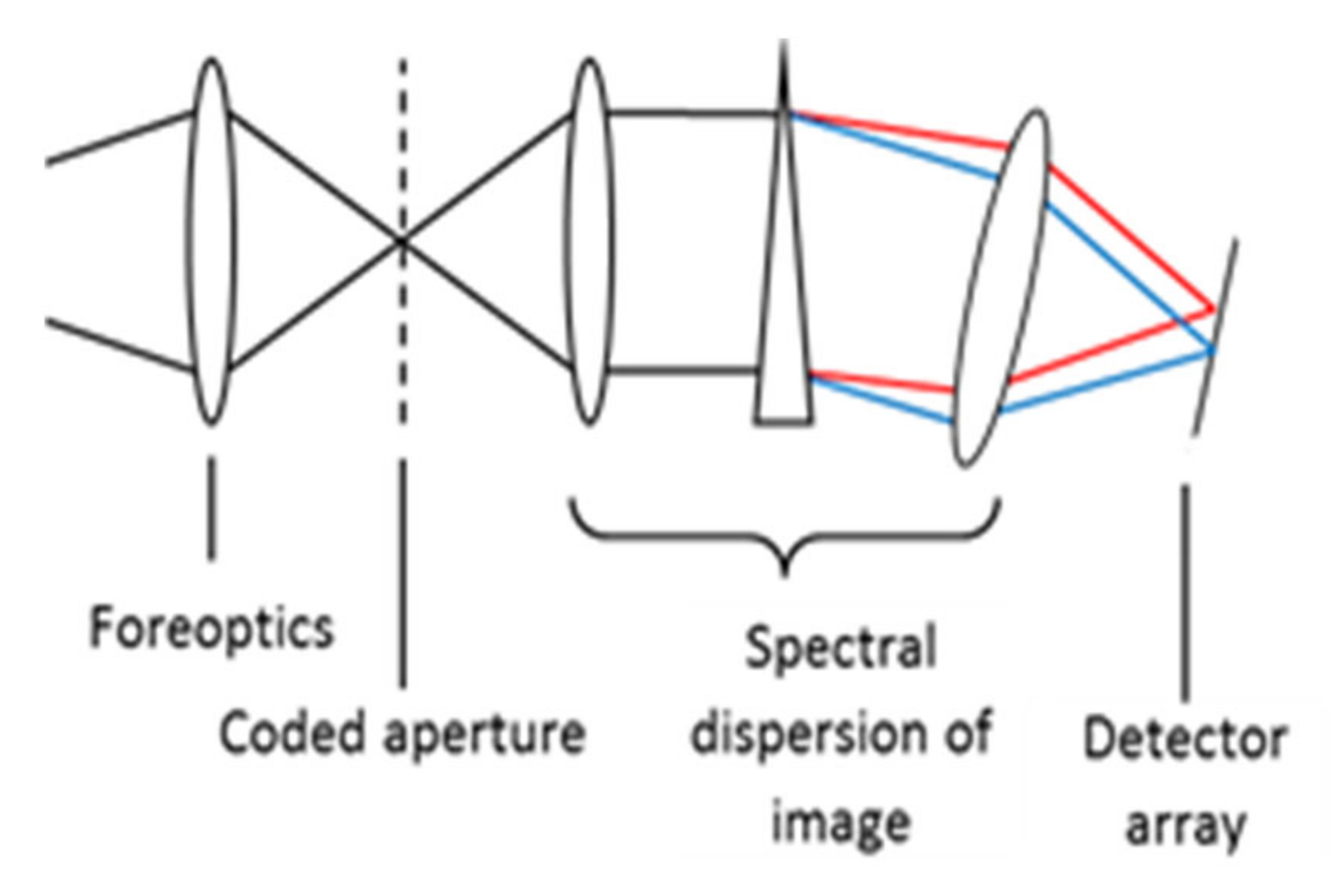
Figure 2.
Illustration of the content of the image as seen by CA multiplexed sensor as depicted in Figure 1. (a) The hyperspectral data cube which consists of two spatial dimensions of x and y, and one spectral dimension, λ. (b) It is then filtered by a code in the undispersed plane such that selected signals at particular spatial locations are allowed to pass through. (c) The optical signal is then dispersed and (d) reimaged onto a detector, which senses the sum of all optical signals of voxels across the wavelength dimension [2].
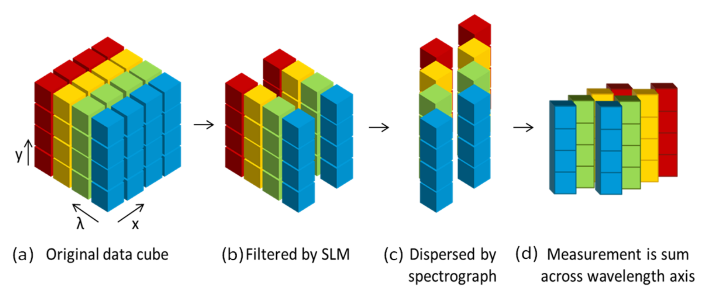
Figure 3.
(a) Examples of the Hadamard matrices of size 8 derived from the quadratic residue construction is adopted here. (b) illustrates the corresponding cyclic binary of the Hadamard matrix. (c) shows an example aperture code that has been utilized in this work. Note that each column of the CA follows the pattern of a column (or row) of a cyclic binary Hadamard matrix. In a practical implementation, this pattern would replace the slit of a conventional pushbroom spectrometer; its width would be a few millimeters and the narrowest feature (transparent row surrounded by opaque rows or opaque row surrounded by transparent rows) would be the same size as a detector pixel (a few microns up to a few tens of microns).
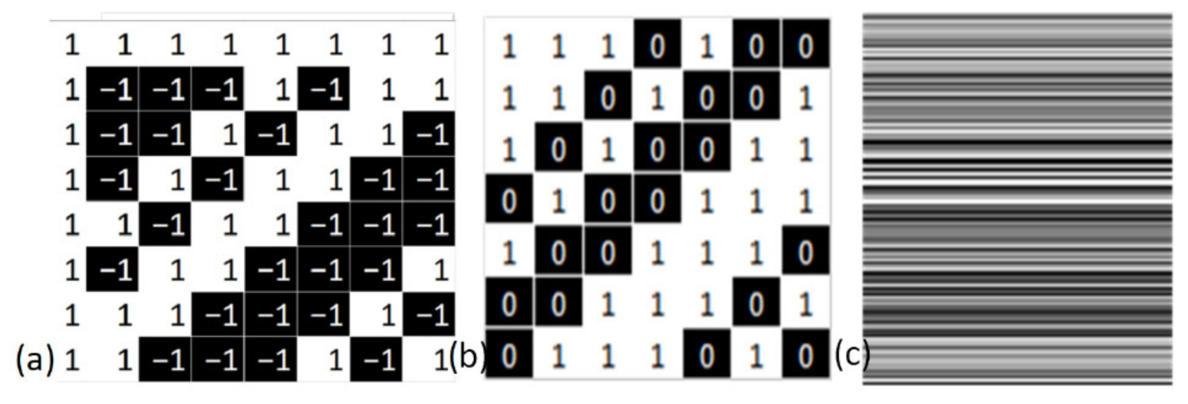
Figure 4.
(a) an example of a 31-band, visible light, airborne hyperspectral image, showing vehicles parked on a concrete pad. (b) Simulation of the central portion of the same image viewed through a sensor of the type considered in this paper. The “blurring” is due to multiple wavelengths overlapping at the focal plane, while some faint horizontal stripes are visible due to the aperture code. Note that multiple frames of this type are required to reconstruct the full hyperspectral image. (c) The aperture code used to simulate (b).

Figure 5.
(a) table illustrating a portion of , showing the indices of each element, with shading to represent an aperture code. The same element of the aperture code is applied to every band from a particular spatial location. (b) table illustrating the spatial arrangement of different elements of after spectral dispersion. Again, shading indicates the pattern of aperture coding applied. The sum of each column (with the value of multiplied by the aperture code) gives the signal at detector element . (c) illustrates which element of the aperture code is applicable to each element in (b).
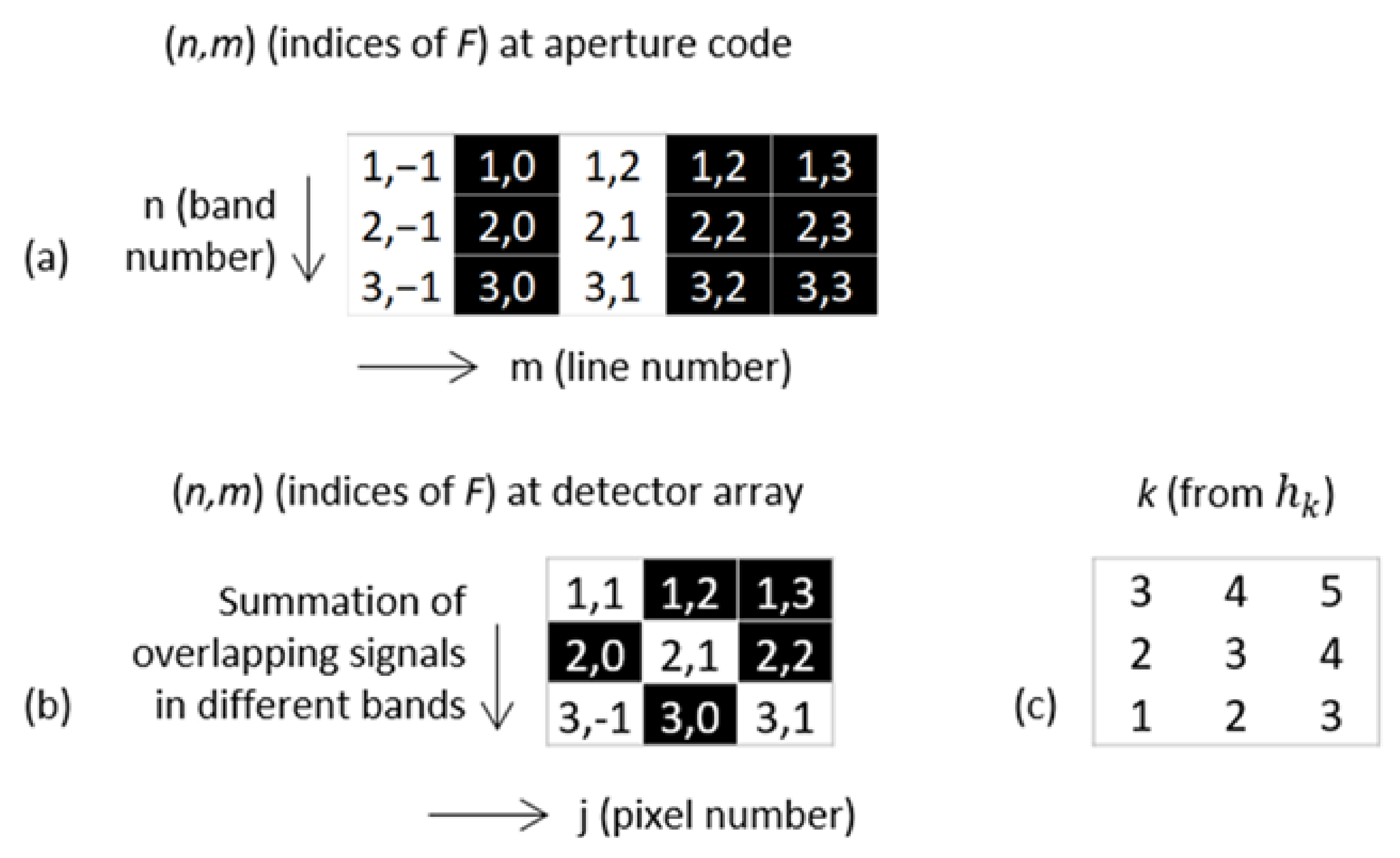
Figure 6.
Depicts the variation of the SNR for the conventional and multiplexed SNRs as a function of wavelength (left) and SNR magnitudes (right), for frame rates at 35 Hz (top) and 200 Hz (bottom). The detector is a Teledyne Chroma array with 480 bands, at low illumination angle of 70° from zenith and f/2.5 optics.

Figure 7.
Depicts the variation of the SNR as a function of frame rate for conventional spectrograph and CA multiplexed sensors under a range of sensing parameters: (a) ground albedo 10% and 60° illumination angle, (b) well depth reduced to 700 K electrons, (c). illumination at 0° from zenith, (d) 120 bands.
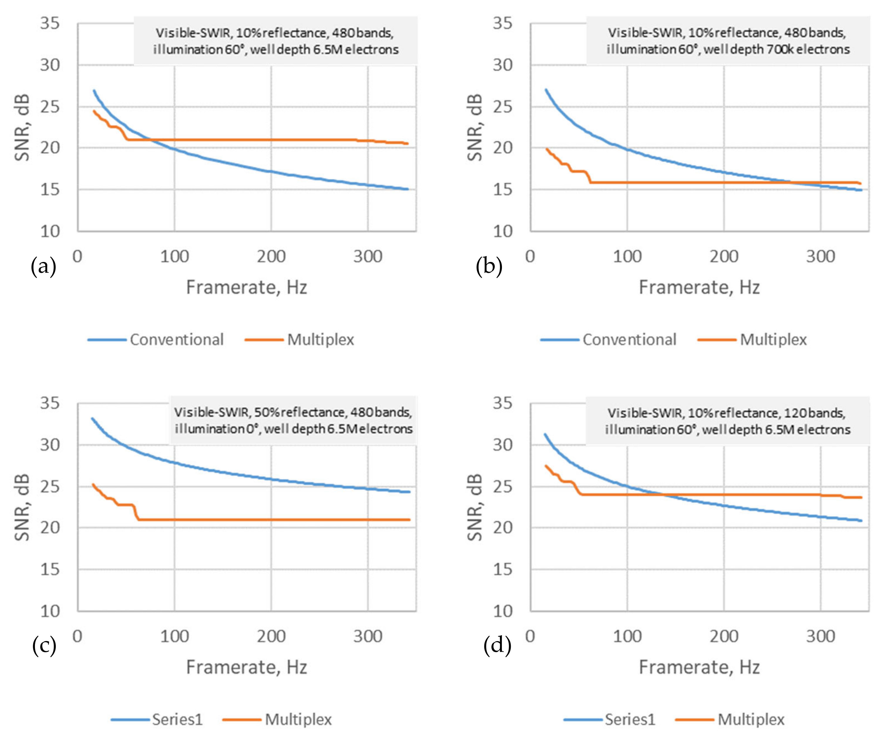
Figure 8.
Shows the SNR behavior of the conventional spectrograph sensing vs. the CA multiplexed sensing for the integrated visible-SWIR sensor system.
Figure 8.
Shows the SNR behavior of the conventional spectrograph sensing vs. the CA multiplexed sensing for the integrated visible-SWIR sensor system.

Figure 9.
Shows the SNR behavior of the conventional spectrograph sensing vs. the CA multiplexed sensing for the SWIR sensing system, at an illumination of 60° zenith.
Figure 9.
Shows the SNR behavior of the conventional spectrograph sensing vs. the CA multiplexed sensing for the SWIR sensing system, at an illumination of 60° zenith.
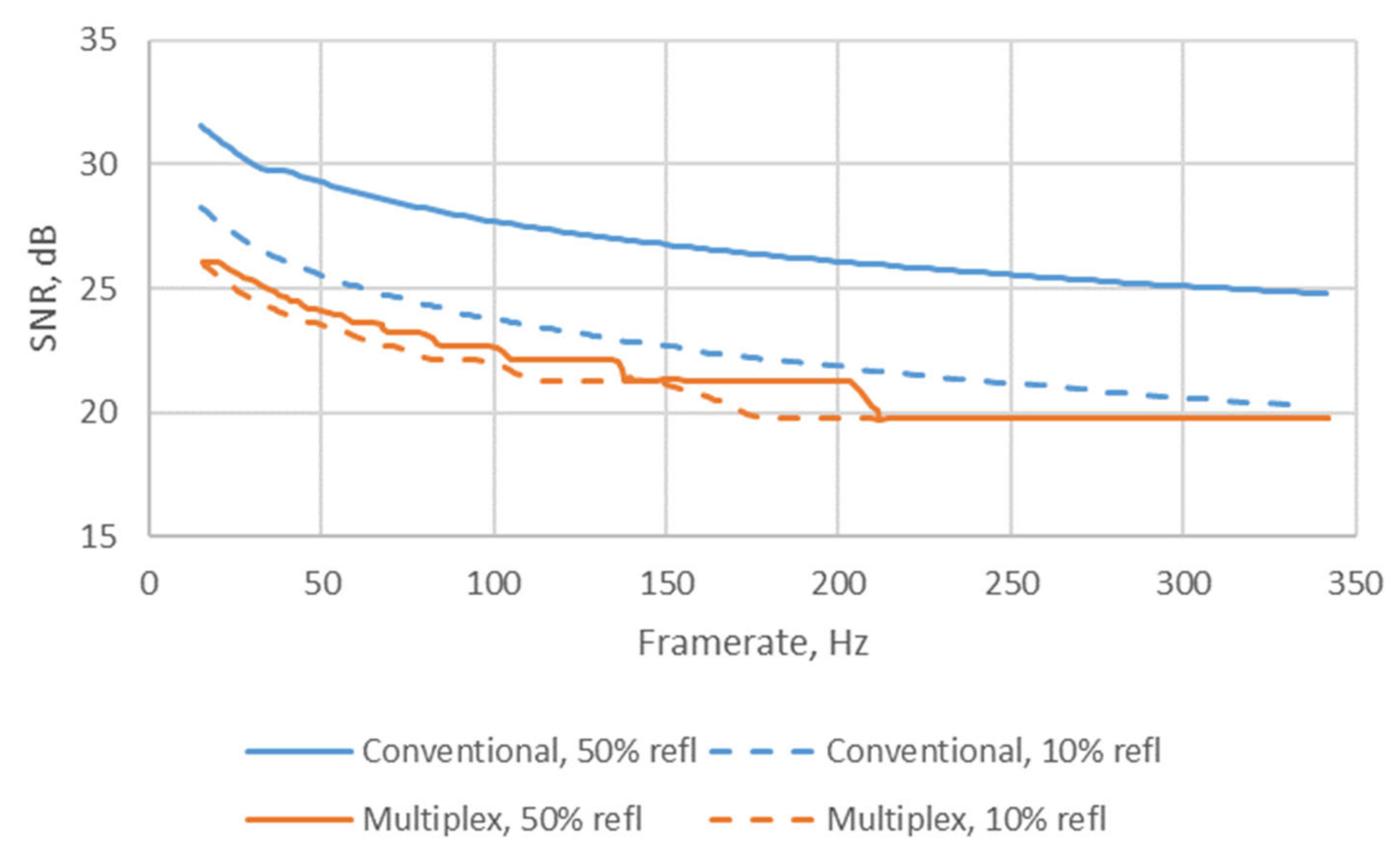
Figure 10.
Shows the SNR behavior of the conventional spectrograph sensing vs. the CA multiplexed sensing for the VNIR sensing system, at an illumination of 60° zenith.
Figure 10.
Shows the SNR behavior of the conventional spectrograph sensing vs. the CA multiplexed sensing for the VNIR sensing system, at an illumination of 60° zenith.


Table 1.
A list of typical sensor characteristics and parameters that have been adopted for the modelled sensors in this work.
Table 1.
A list of typical sensor characteristics and parameters that have been adopted for the modelled sensors in this work.
| Modelled Sensor Parameters | Visible-SWIR | SWIR Band | Visible-NIR |
|---|---|---|---|
| No. of wavebands | 480.0 | 288.0 | 768.0 |
| Pixel sizes, µm | 30.0 | 20.0 | 8.0 |
| Pixel well depth, e− | 5.0 × 10⁶ | 1.10 × 10⁶ | 9.0 × 10⁴ |
| Noise floor level, e− | 600.0 | 150.0 | 110.0 |
| Dark current level, e−/s/pixel | 207.0 | 100.0 | 4000.0 |
| Max. frame rate, Hz | 125.0 | 450.0 | 170.0 |
| Readout time, µs | 16.80 | 7.70 | -- |
| Optical throughput f/# | 2.00 | 2.00 | 2.50 |
Publisher’s Note: MDPI stays neutral with regard to jurisdictional claims in published maps and institutional affiliations. |
© 2022 by the authors. Licensee MDPI, Basel, Switzerland. This article is an open access article distributed under the terms and conditions of the Creative Commons Attribution (CC BY) license (https://creativecommons.org/licenses/by/4.0/).
Share and Cite
MDPI and ACS Style
Piper, J.; Yuen, P.W.T.; James, D. Signal to Noise Ratio of a Coded Slit Hyperspectral Sensor. Signals 2022, 3, 752-764. https://doi.org/10.3390/signals3040045
AMA Style
Piper J, Yuen PWT, James D. Signal to Noise Ratio of a Coded Slit Hyperspectral Sensor. Signals. 2022; 3(4):752-764. https://doi.org/10.3390/signals3040045
Chicago/Turabian StylePiper, Jonathan, Peter W. T. Yuen, and David James. 2022. "Signal to Noise Ratio of a Coded Slit Hyperspectral Sensor" Signals 3, no. 4: 752-764. https://doi.org/10.3390/signals3040045