An Overview of Mathematical Methods Applied in the Biomechanics of Foot and Ankle–Foot Orthosis Models

Abstract

Ankle–foot orthoses (AFOs) constitute medical instruments designed for patients exhibiting pathological gait patterns, notably stemming from conditions such as stroke, with the primary objective of providing support and facilitating rehabilitation. The present research endeavors to conduct a comprehensive review of extant scholarly literature focusing on mathematical techniques employed for the examination of AFO models. The overarching aim is to gain deeper insights into the biomechanical intricacies underlying these ankle–foot orthosis models from a mathematical perspective, while concurrently aiming to advance novel models within the domain. Utilizing a specified set of keywords and their configurations, a systematic search was conducted across notable academic databases, including ISI Web of Knowledge, Google Scholar, Scopus, and PubMed. Subsequently, a total of 23 articles were meticulously selected for in-depth review. These scholarly contributions collectively shed light on the utilization of nonlinear optimization techniques within the context of ankle–foot orthoses (AFOs), specifically within the framework of fully Cartesian coordinates, encompassing both kinematic and dynamic dimensions. Furthermore, an exploration of a two-degree-of-freedom AFO design tailored for robotic rehabilitation, which takes into account the interplay between foot and orthosis models, is delineated. Notably, the review article underscores the incorporation of shape memory alloy (SMA) elements in AFOs and overviews the constitutive elastic, viscoelastic, and hyperelastic models. This comprehensive synthesis of research findings stands to provide valuable insights for orthotists and engineers, enabling them to gain a mathematical understanding of the biomechanical principles underpinning AFO models and fostering the development of innovative AFO designs.

1. Introduction

Ankle–foot orthoses (AFOs) represent orthotic apparatus employed in the management of patients afflicted with aberrant gait patterns [1]. Their primary role is to provide assistance to individuals exhibiting pathological gait and to facilitate the process of rehabilitation [2]. In the context of ambulation, the term “gait cycle” is defined as the duration between two identical events commencing from the initial heel strike and culminating in the repetition of the same event for the same foot [3]. The biomechanics of this movement could be a first step in the process used in the design of ankle–foot orthoses. With new technological developments, it has been observed that for professionals in engineering biomechanics, the analysis of human movement provides crucial detailed quantitative data [4]. Human motion analysis involves the utilization of intricate theoretical and computational techniques aimed at elucidating the kinematic and dynamic aspects of human locomotion [5,6]. Recognizing the inherent interplay between kinematics, muscle activity, and kinetic parameters, such information has been deemed indispensable for a more comprehensive comprehension of alterations in gait patterns [7]. Dynamic analysis involves the comprehensive examination of motion within a multibody system, encompassing considerations of the external forces acting upon it, as well as its inherent inertial properties. A subset of these external forces is computed by solving the system’s equations of motion, while others necessitate empirical acquisition [8]. Within the domain of dynamic analysis, two primary problem categories emerge: forward and inverse dynamics [9]. In the case of the inverse dynamic problem, it is imperative to initially gather kinematic data and ground reaction force (GRF) information [10]. Forward dynamic analysis entails the simulation of the multibody system’s motion over a specified time interval, integrating applied forces and initial conditions [9]. In contrast, the inverse problem pertains to the determination of the dynamic forces and moments responsible for a specific motion in conjunction with the reactions occurring at each joint [11].

The resolution of inverse and forward dynamics necessitates the establishment of a biomechanical model, serving as a mathematical approximation of the actual biological system derived from external data, anthropometric parameters, and the system’s equations of motion [12,13,14]. A multibody system approach is employed to simulate the kinematic and dynamic environment of the system. This system comprises two or more interconnected rigid bodies with kinematic joints facilitating their motion, subjected to external forces [15]. The degrees of freedom afforded by the kinematic joint configuration determine the nature of motion, introducing constraints on relative movement between the rigid bodies [16]. This article’s overarching objective lies in scrutinizing the existing literature to investigate mathematical methodologies applied to the analysis of ankle–foot orthoses (AFO) models. The insights gleaned from this review are poised to be of significant value to orthotists and engineers, who can leverage this information to establish a mathematical understanding of the biomechanical principles underpinning AFO models and explore avenues for the development of innovative models.

2. Methods

2.1. Search Strategy

The protocol type that is used in this study is the ‘‘search protocol’’. This protocol outlines the search strategy used to identify relevant studies for this review. It includes the databases searched, search terms used, and inclusion and exclusion criteria.

A comprehensive literature search was undertaken by querying databases such as Scopus, Google Scholar, ISI Web of Knowledge, and PubMed, spanning a time frame from 1990 to 2023. The selection of keywords employed in this systematic search process is elaborated upon below: “ankle–foot orthosis (AFO)”, “numerical methods”, “biomechanics”, “mathematical model”, “constitutive methods”, “kinetic”, “kinematics”, and “dynamic”.

2.2. Study Selection

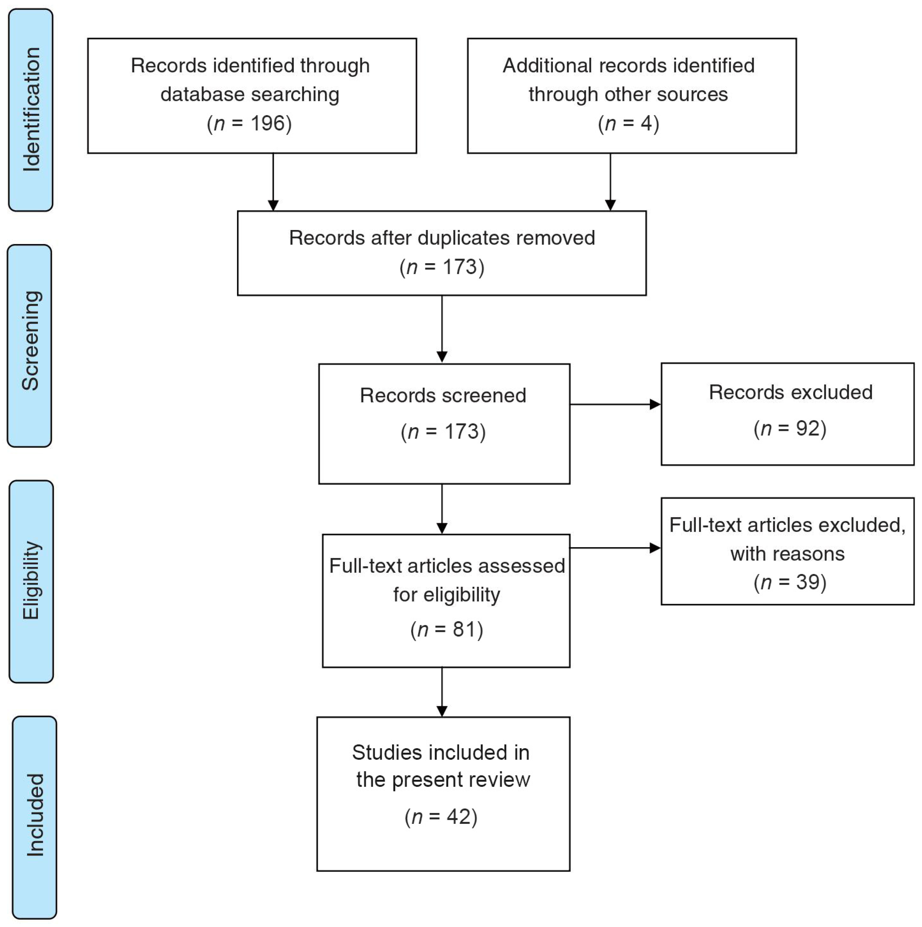
A PRISMA (Preferred Reporting Items for Systematic reviews and Meta-Analyses) flowchart template was used for the selection of studies, and the result of this process is illustrated in Figure 1. Initially, for 196 articles, we screened titles and abstracts to identify potentially relevant articles. Subsequently, full-text reviews were conducted according to predetermined inclusion and exclusion criteria. The final selection process resulted in 42 full-text articles.

Inclusion criteria included articles in which:

• Studies considered for inclusion were numerical and not experimental or clinical studies alone;
• The means of analysis, such as equations, parameters, and methods, were clearly explained;
• The study was written in English and published in a peer-reviewed journal.

Consistent with PRISMA guidelines, we conducted a rigorous process of data extraction. However, regarding the other PRISMA elements, such as the data synthesis and the assessment of bias, they were not relevant in our review.

3. Results and Discussions

3.1. Nonlinear Optimization Function

3.1.1. Fully Cartesian Coordinates

Prior to embarking on the modeling of a system’s motion within a three-dimensional space, the selection of an appropriate coordinate system becomes a pivotal prerequisite, given the array of choices available for representing a multibody system [17]. This entails the utilization of unit vectors denoting joint axis rotations, presented as a column vector q, alongside a collection of points positioned at either the extremities or the articulation points within the model, collectively facilitating the representation of fully Cartesian coordinates:

$$q={\left\{{\mathrm{x}}_{\mathrm{P}1}{\mathrm{y}}_{\mathrm{P}1}{\mathrm{z}}_{\mathrm{P}1}\dots {\mathrm{x}}_{\mathrm{P}\mathrm{n}}{\mathrm{y}}_{\mathrm{P}\mathrm{n}}{\mathrm{z}}_{\mathrm{P}\mathrm{n}}{\mathrm{x}}_{\mathrm{V}1}{\mathrm{y}}_{\mathrm{V}1}{\mathrm{z}}_{\mathrm{V}1}\dots {\mathrm{x}}_{\mathrm{V}\mathrm{m}}{\mathrm{y}}_{\mathrm{V}\mathrm{m}}{\mathrm{z}}_{\mathrm{V}\mathrm{m}}\right\}}^{\mathrm{T}}$$

(1)

where V stands for vectors, P stands for points, m and n are, respectively, the number of vectors and points used to model the system.

The vector composed of generalized coordinates serves as a fundamental representation of a system. The total count of these coordinates is equivalent to the number of elements within the vector, defined by the following equation:

$$nc=3(n+m).$$

(2)

The ensemble of six coordinates comprises a trinity of orientation coordinates, which meticulously detail the spatial orientation of the system, and an additional trio of positional coordinates, meticulously pinpointing the precise location of the system concerning a static reference frame. It is of paramount importance to acknowledge that the nature of these coordinates may exhibit either a dependent or an independent character. The independent coordinates are intrinsically contingent upon the inherent degrees of freedom embedded within the system. In contrast, dependent coordinates emerge when their numerical abundance surpasses the degrees of freedom at the disposal of the system. The essence of these kinematic constraints is succinctly encapsulated within the ensuing column vector:

$$\Phi (q,t)=\left\{\begin{array}{c}{\Phi }^{RBC}\left(q\right)\hfill \\ {\Phi }^{JC}\left(q\right)=0\hfill \\ {\Phi }^{DC}(q,t)\hfill \end{array}\right.,$$

(3)

where RBCs are the rigid body characteristics, DCs are the kinematic drivers, and JCs are the joint kinematics of the system.

For a rigid body free from spatial constraints, it possesses six degrees of freedom, comprising three rotational and three translational degrees of freedom [18]. The enumeration of degrees of freedom within a mechanical system corresponds to the overall count of generalized coordinates essential for elucidating the system’s behavior. This tally is discerned by subtracting the number of constraints introduced by the presence of kinematic joints in the system. In essence, the degrees of freedom encapsulate the system’s capacity for independent motion, while constraints restrict and define the permissible range of such motion, forming a pivotal aspect of mechanical system analysis [19].

3.1.2. Kinematic Analysis

This analysis pertains to the study of motion, irrespective of the forces instigating it, and is sometimes referred to as the “initial position problem”. The nomenclature aligns with the task of determining the positions of all components within the system, factoring in the input provided by driving constraints [20]. From a mathematical perspective, this entails determining the generalized coordinates (q) that satisfy the set of kinematic constraint equations at each time step of the analysis, described as follows:

$$\Phi (q,t)=0.$$

(4)

To solve Equation (3), the Newton–Raphson method (NRN) is employed, known for its quadratic convergence properties near the solution [21], achieved by linearizing the system at $q_i$:

$$\Phi (q,t)\cong \Phi \left(q_i\right)+{\Phi }_{\mathrm{q}}\left(q_i\right)\left(q-q_i\right)=0.$$

(5)

The resolution for the partial derivatives of each kinematic constraint concerning the vector of generalized coordinates finds its representation in the form of the Jacobian matrix of constraints, denoted as ${\Phi }_{\mathrm{q}}\left(q_i\right)$, as stipulated in Equation (6):

$${\Phi }_{\mathrm{q}}\left(q_i\right)=\left[\begin{array}{ccc}\frac{\partial {\Phi }_1}{\partial {\mathrm{q}}_{\mathrm{n}1}}& \cdots & \frac{\partial {\Phi }_1}{\partial {\mathrm{q}}_{\mathrm{n}\mathrm{c}}}\\ ⋮& \ddots & ⋮\\ \frac{\partial {\Phi }_{\mathrm{n}\mathrm{h}}}{\partial {\mathrm{q}}_{\mathrm{n}1}}& \cdots & \frac{\partial {\Phi }_{\mathrm{n}\mathrm{h}}}{\partial {\mathrm{q}}_{\mathrm{n}\mathrm{c}}}\end{array}\right],$$

(6)

where nc denotes the number of dependent coordinates and nh signifies the count of constrained equations.

The vector representing an approximation of the correct system position is derived as the solution to Equation (4). An iterative equation, denoted as $q_{i+1}$, is established as follows:

$$\Phi \left(q_i\right)+{\Phi }_q\left(q_i\right)\left(q_{i+1}-q_i\right)=0.$$

(7)

To determine the system’s velocity, one simply needs to differentiate the kinematic constraint Equation (4) with respect to time, which results in the following expression:

$$\Phi (q,\dot{q},\mathrm{t})=\frac{\mathrm{d}\Phi (q,\mathrm{t})}{\mathrm{d}\mathrm{t}}=\frac{\partial q}{\partial \mathrm{t}}\frac{\partial \Phi (q,\mathrm{t})}{\partial \mathrm{t}}+\frac{\partial \Phi (q,\mathrm{t})}{\partial q}=0,$$

(8)

where $\frac{\partial \Phi \left(q,\mathrm{t}\right)}{\partial \mathrm{t}}$ represents the vector $v\left(t\right)$, consisting of the partial derivatives of Φ with respect to time; $\frac{\partial \Phi (q,\mathrm{t})}{\partial q}$ signifies the Jacobian matrix, and $\frac{\partial q}{\partial \mathrm{t}}$ represents the vector of generalized velocities, $\dot{q}$. Thus, the velocity equation is articulated as:

$${\Phi }_q\dot{q}=v\left(t\right).$$

(9)

Differentiating the constraint velocities from Equation (8) with respect to time yields the vector of constraint accelerations:

$$\ddot{\Phi }(q,\dot{q},\ddot{q},t)=\frac{d\dot{\Phi }(q,\dot{q},t)}{dt}={\Phi }_q\ddot{q}+{\left({\Phi }_q\dot{q}\right)}_q\dot{q}+v_t=0.$$

(10)

Since the vector $\gamma \left(q,\dot{q},t\right)$is defined as:

$$\gamma (q,\dot{q},t)=v_t-{\left({\Phi }_q\dot{q}\right)}_q\dot{q},$$

(11)

then, the acceleration equation results in:

$${\Phi }_q\ddot{q}=\gamma .$$

(12)

3.1.3. Dynamic Analysis

To tackle the dynamic analysis problem for a multibody system, it is imperative to possess a comprehensive understanding of the external inertia and forces acting upon each individual rigid body within the system [22]. Several methods can be employed to derive the equations of motion, with one of them being the principle of virtual power, as presented below. In this principle, the sum of the virtual power generated by the external forces at each moment equates to zero [16]:

$$P^{*}={\sum }_{i=1}^{nc} f_i{\dot{q}}_i^{*}\equiv {\dot{q}}_i^{*T}f=0,$$

(13)

where, the vector f, representing all the forces generating virtual power, is expressed as:

$$f=M\ddot{q}-g.$$

(14)

In the context of the equation set, $M\ddot{q}$represents the vector signifying the inertial forces, where M denotes the comprehensive global mass matrix and $\ddot{q}$ symbolizes the vector delineating generalized accelerations. Simultaneously, $g$ stands as the vector encompassing generalized applied forces. It is noteworthy that the internal forces, organized in action–reaction pairs, do not contribute to the concept of virtual power and, therefore, are not factored into Equation (13). Nevertheless, their determination is attainable through the utilization of the Lagrange multiplier technique, presented as follows:

$$g^{\Phi }={\Phi }_{\mathrm{q}}^{\mathrm{T}}\lambda .$$

(15)

In this equation, $g^{\Phi }$ designates the vector characterizing generalized forces, while $\lambda$ constitutes the column vector housing the Lagrange multipliers. The magnitude of these internal constraint forces is ascertained through these multipliers, whereas their specific direction is contingent on the information encoded in the Jacobian matrix. The equation encapsulating the concept of virtual power is deduced by amalgamating the expressions found in Equations (13)–(15):

$$P^{*}={\dot{q}}^{*T}\left(M\ddot{q}-g+{\Phi }_q^T\lambda \right)=0.$$

(16)

The holistic equation of motion, presented comprehensively below, serves as the cornerstone to unearth the system’s unknown variables:

$$\left\{\begin{array}{c}M\ddot{q}+{\Phi }_q^T\lambda =g\\ {\Phi }_q\ddot{q}=\gamma \end{array}\right..$$

(17)

This method proves to be instrumental in bringing together and solving the equations of motion (17) for the biomechanical system. Depending on the selected approach for solving these equations, researchers can engage in either forward dynamic analysis (Simulation) or inverse dynamic analysis. The latter, in particular, plays a pivotal role in deducing the external forces governing the observed motion, thereby unveiling the hitherto unknown external and internal forces. This analytical approach yields invaluable results, significantly contributing to the field [23].

3.2. Two-Degree-of-Freedom AFO for Robotic Rehabilitation

The capability of accommodating eversion–inversion motion in ankle–foot orthoses is contingent on the flexibility of the material employed. However, constraints on the normal eversion–inversion range contribute to discomfort and hinder the emulation of a natural ankle motion [24]. In this context, the discussion centers on an ankle–foot orthosis (AFO) endowed with two degrees of freedom. These degrees of freedom encompass plantarflexion–dorsiflexion and eversion–inversion motions. Notably, the plantarflexion–dorsiflexion motion is actively regulated by a DC servomotor, whereas the eversion–inversion joint operates passively, facilitated by a damper and a torsion spring. The latter components are instrumental in restricting the range of motion beyond a specific threshold by applying spring force [25].

3.2.1. Model of the Foot

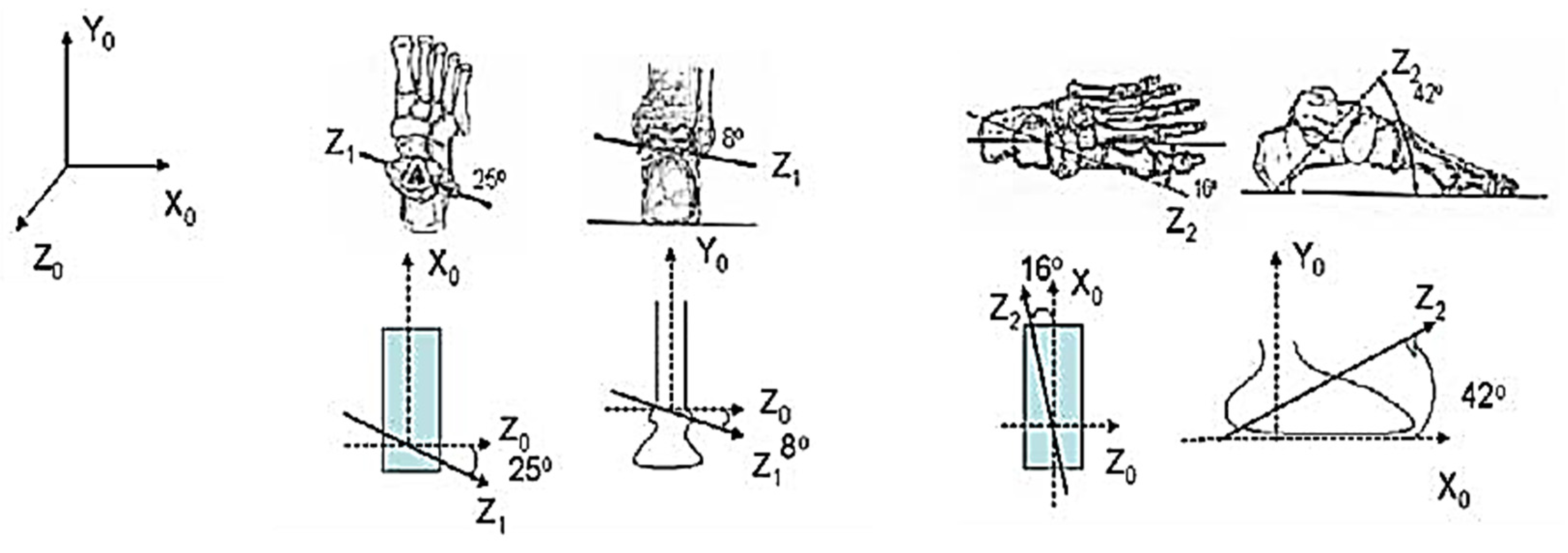
The intricate motion of the foot is a multifaceted process that transpires across three distinct planes and revolves around three separate axes [26]. The orientations of the remaining two joint axes and the mapping of these joint axes onto the inertial frame are integral components of this intricate movement and are depicted in Figure 2. The inertial frame is affixed to the axis and the shank, ensuring a stable reference frame [27].

It is pertinent to note that ${\overrightarrow{Z}}_0$ symbolizes the knee joint axis, ${\overrightarrow{Z}}_1$ denotes the plantarflexion–dorsiflexion joint axis, and ${\overrightarrow{Z}}_2$ represents the eversion–inversion joint axis. These axes are considered when the foot is in firm contact with the ground and the shank is perpendicular to the ground, thus setting the reference projection. Sequential rotations are essential to transition from ${\overrightarrow{Z}}_0$ to ${\overrightarrow{Z}}_1$ and subsequently from ${\overrightarrow{Z}}_1$ to ${\overrightarrow{Z}}_2$, facilitating the determination of rotation matrices required to reach the desired frame.

The representation relies on spherical coordinates, which are inherently linked to Cartesian coordinates as follows:

$$[x,y,z]=[r\mathrm{c}\mathrm{o}\mathrm{s} \gamma \mathrm{s}\mathrm{i}\mathrm{n} \varphi ,r\mathrm{s}\mathrm{i}\mathrm{n} \gamma \mathrm{s}\mathrm{i}\mathrm{n} \varphi ,r\mathrm{c}\mathrm{o}\mathrm{s} \varphi ].$$

(18)

The three Z vectors within the inertial frame can be expressed as follows:

$${\overrightarrow{Z}}_0=[\mathrm{0,0},1],$$

(19)

$${\overrightarrow{Z}}_1=\left[\mathrm{c}\mathrm{o}\mathrm{s} {\gamma }_1\mathrm{s}\mathrm{i}\mathrm{n} {\varphi }_1,\mathrm{s}\mathrm{i}\mathrm{n} {\gamma }_1\mathrm{s}\mathrm{i}\mathrm{n} {\varphi }_1,\mathrm{c}\mathrm{o}\mathrm{s} {\varphi }_1\right],$$

(20)

$${\overrightarrow{Z}}_2=\left[\mathrm{c}\mathrm{o}\mathrm{s} {\gamma }_2\mathrm{s}\mathrm{i}\mathrm{n} {\varphi }_2,\mathrm{s}\mathrm{i}\mathrm{n} {\gamma }_2\mathrm{s}\mathrm{i}\mathrm{n} {\varphi }_2,\mathrm{c}\mathrm{o}\mathrm{s} {\varphi }_2\right].$$

(21)

The angles $\gamma$ and $\varphi$ can be calculated based on the projection of joint axes in the inertial frame. The projections of the ${\overrightarrow{Z}}_i$ axis in the inertial frame are represented as ($X^{i^{\prime }},Y^{i^{\prime }},Z^{i^{\prime }}$) for i = 1, 2, and can be determined using the following equations:

$${\gamma }_i=\mathrm{A}\mathrm{t}\mathrm{a}\mathrm{n} 2\left(Y^{i^{\prime }},X^{i^{\prime }}\right),$$

(22)

$${\varphi }_i=\mathrm{A}\mathrm{t}\mathrm{a}\mathrm{n} 2\left(\frac{Y^{i^{\prime }}}{\sin {\gamma }_i},Z^{i^{\prime }}\right).$$

(23)

Once the orientations of ${\overrightarrow{Z}}_1$ and ${\overrightarrow{Z}}_2$ in the inertial frame are established, the Denavit–Hartenberg parameters can be computed, allowing for the formulation of rotation matrices by defining the ${\overrightarrow{X}}_1$, ${\overrightarrow{Y}}_1$ axes and ${\overrightarrow{X}}_2$, ${\overrightarrow{Y}}_2$ axes as follows:

$${\overrightarrow{X}}_{i+1}=\frac{{\overrightarrow{Z}}_i\times {\overrightarrow{Z}}_{i+1}}{∥{\overrightarrow{Z}}_i\times {\overrightarrow{Z}}_{i+1}∥},$$

(24)

$${\overrightarrow{Y}}_{i+1}=\frac{{\overrightarrow{Z}}_{i+1}\times {\overrightarrow{X}}_{i+1}}{∥{\overrightarrow{Z}}_{i+1}\times {\overrightarrow{X}}_{i+1}∥}.$$

(25)

The Denavit–Hartenberg parameters ${\theta }_i$, ${\alpha }_i$, $a_i,$ and $d_i$ are then calculated for the transformation of frames $f_i$ to frame $f_{i+1}$ [28]. The transformation matrix can be represented as:

$$T_i^{i+1}=\left(\begin{array}{cccc}\mathrm{c}\mathrm{o}\mathrm{s} {\theta }_i& -\mathrm{c}\mathrm{o}\mathrm{s} {\alpha }_i\mathrm{s}\mathrm{i}\mathrm{n} {\theta }_i& \mathrm{s}\mathrm{i}\mathrm{n} {\alpha }_i\mathrm{s}\mathrm{i}\mathrm{n} {\theta }_i& a_i\mathrm{c}\mathrm{o}\mathrm{s} {\theta }_i\\ \mathrm{s}\mathrm{i}\mathrm{n} {\theta }_i& \mathrm{c}\mathrm{o}\mathrm{s} {\alpha }_i\mathrm{c}\mathrm{o}\mathrm{s} {\theta }_i& -\mathrm{s}\mathrm{i}\mathrm{n} {\alpha }_i\mathrm{c}\mathrm{o}\mathrm{s} {\theta }_i& a_i\mathrm{s}\mathrm{i}\mathrm{n} {\theta }_i\\ 0& \mathrm{s}\mathrm{i}\mathrm{n} {\alpha }_i& \mathrm{c}\mathrm{o}\mathrm{s} {\alpha }_i& d_i\\ 0& 0& 0& 1\end{array}\right).$$

(26)

The position loop closure equation is used to find the $a_i$ and $d_i$:

$$T_0^3=T_0^1{T}_1^2{T}_2^3.$$

(27)

In this equation, $T_0^3$ is computed independently using ${\overrightarrow{Z}}_1$and ${\overrightarrow{Z}}_3$. The parameters $a_0,d_0,d_1,a_2,$and $d_2$ are assumed based on the foot’s geometry, while $a_1,a_3,{\mathrm{a}\mathrm{n}\mathrm{d} d}_3$ are calculated from three equations obtained from the previous loop closure equation. The complete kinematic model becomes known once all these parameters are determined.

Leveraging the assistance of the kinematic model, one can proceed to formulate the dynamic model, which, in turn, streamlines the process of designing the orthosis. The dynamic model of the system operates under the framework of the Lagrangian formulation and assumes a fixed shank, simplifying the overall analysis. This formulation is derived from the potential and kinetic energies of the system. As additional springs and masses are integrated into the system, the dynamic model must be adjusted to accurately represent the potential and kinetic energies of the system. The equations of motion are expressed as:

$$D\left(q\right)\ddot{q}+C(q,\dot{q})\dot{q}+G\left(q\right)=\tau .$$

(28)

Here, $D\left(q\right)$ denotes the (2 × 2) inertia matrix, $C(q,\dot{q})$ represents the (2 × 2) terms for Coriolis and centrifugal effects, $G\left(q\right)$ stands for the (2 × 1) vector of gravity torque, and $q={\left[{\theta }_1,{\theta }_2\right]}^T$ is the vector encompassing all joint variables.

3.2.2. Model of the Orthosis

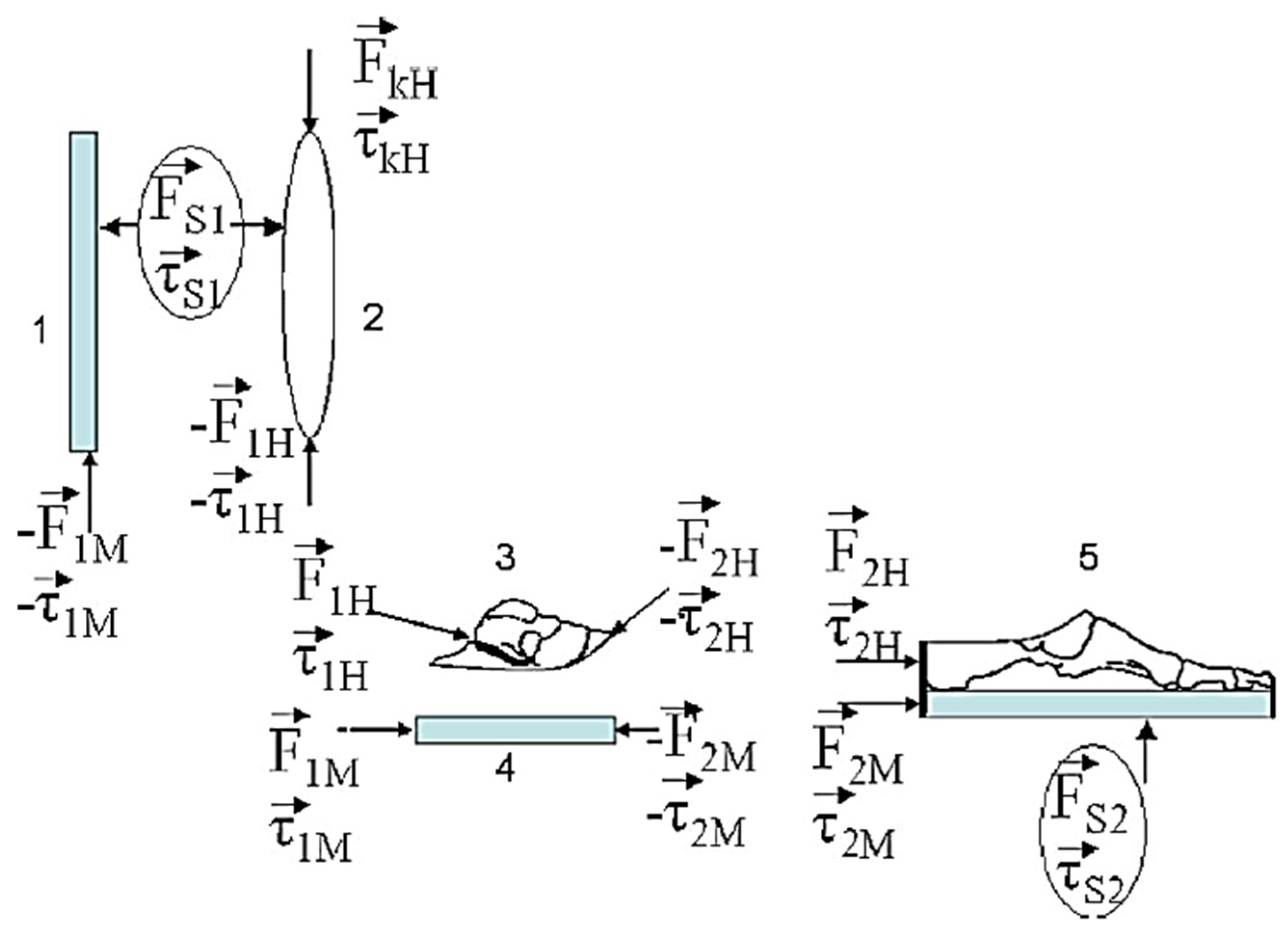
Figure 3 depicts the free-body diagram of all the components within the system. The machine segments are represented by rectangular shapes, while the human segments are denoted by bony and oval shapes. The weight of each body acts at its center of mass. Sensor forces and torques are illustrated by circles. The subscripts M correspond to the machine components, H to the human components, and S signifies the sensor component. ${\overrightarrow{F}}_{kH}$and ${\overrightarrow{\tau }}_{kH}$ represent the force and torque applied at the knee joint.

Once the complete motion of the system is known through the Newton–Euler equations, and the force–torque sensors provide ${\overrightarrow{F}}_{S1},{\overrightarrow{\tau }}_{S1} \mathrm{and} {\overrightarrow{F}}_{S2},{\overrightarrow{\tau }}_{S2}$, the remaining unknowns can be uniquely determined. The set-point control of the ankle–foot orthosis is a noteworthy aspect of this underactuated system, characterized by the presence of a damper and a spring at the passive eversion–inversion joint, is represented in Equation (28) and can be expressed as:

$$\left(\begin{array}{cc}{d}_{11}& d_{12}\\ d_{21}& d_{22}\end{array}\right)\left[\begin{array}{c}{\ddot{\theta }}_1\\ {\ddot{\theta }}_2\end{array}\right]+\&\left(\begin{array}{cc}{c}_{11}& c_{12}\\ c_{21}& c_{22}\end{array}\right)\left[\begin{array}{c}{\dot{\theta }}_1\\ {\dot{\theta }}_2\end{array}\right]+\left[\begin{array}{c}{g}_1\\ g_2\end{array}\right]\&+\left[\begin{array}{c}0\\ K_t{\theta }_2+K_{td}{\dot{\theta }}_2\end{array}\right]=\left[\begin{array}{c}\tau \\ 0\end{array}\right]$$

(29)

Therefore, it is imperative to verify the stability of the control law for the system. This is achieved by defining a Lyapunov function, V_L, as the total energy of the system, along with an additional error term:

$$V_L=\frac{1}{2}{\dot{q}}^{T}D\dot{q}+V_0+V_m+\frac{1}{2}{K}_t{\theta }_2^2+\frac{1}{2}{K}_p{e}_1^2.$$

(30)

Within this equation, $V_m$ represents the potential energy attributed to gravity, $K_p$ is a positive constant, and $e_1={\theta }_1-{\theta }_{1d}$ signifies the error associated with the first joint. Moreover, $V_0$ is another positive constant ensuring that $V_L$ > 0 remains greater than zero. The primary aim here is to establish that throughout any trajectory of the system, the function $V_L$ steadily decreases, eventually converging to zero. This phenomenon implies that the machine is progressively advancing towards the desired configuration denoted as $q_d$. Assuming a constant $q_d$ and making use of the properties of a skew-symmetric matrix, specifically, ${\dot{q}}^T(\dot{D}-2C)\dot{q}$, being equal to zero, the application of Equations (29) and (30), in conjunction with the time derivative of V_L, leads to the formulation of the ensuing equation:

$${\dot{V}}_L={\dot{\theta }}_1\left(\tau +K_p{e}_1\right)-K_{td}{\dot{\theta }}_2^2.$$

(31)

Here, K_td is the damping coefficient. By selecting a PD control law $=-K_p{e}_1-K_d{\dot{\theta }}_1$:

$${\dot{V}}_L=-K_d{\dot{\theta }}_1^2-K_{td}{\dot{\theta }}_2^2.$$

(32)

The analysis demonstrates that V_L decreases as long as ${\dot{\theta }}_1$, ${\dot{\theta }}_2$ are non-zero. By applying LaSalle’s theorem, ${\dot{V}}_L=0$ implies $\dot{q}$ = 0 and, consequently, ${\ddot{q}}_1$= 0. Using the equations of motion with the control $\tau =-K_p{e}_1-K_d{\dot{\theta }}_1$, Equation (29) becomes:

$$\left[\begin{array}{c}{g}_1+K_p{e}_1\\ g_2+K_t{\theta }_2\end{array}\right]=0.$$

(33)

K_p can be selected to be sufficiently large to drive $e_1$ close to zero, causing ${\dot{\theta }}_1$ to approach the desired set point.

The control torque is provided by the actuator within the simulation, although it is important to acknowledge that, in practical human use, an internal torque will also be generated by the muscles. In such instances, the net torque required by the actuator is determined by the equation:

$${\tau }_M+{\tau }_H=-K_p{e}_1-K_d{\dot{\theta }}_1.$$

(34)

Here, ${\tau }_M$ represents the machine component of the torque, while ${\tau }_M$ signifies the human component. ${\tau }_M$ can be ascertained in real-time using force-torque sensor data. Once ${\tau }_M$ is known, it allows for the calculation of the necessary motor torque based on Equation (34).

3.3. SMA-Element-Based AFO

Various methodologies have been introduced to model the behavior of shape memory alloys (SMAs). One of the models, proposed by Brinson and Huang, segregates the martensite volume (ξ) into two distinct components: temperature-induced martensitic (ξ_T) and stress-induced martensitic (ξ_S) [29]. To delineate ξ_S and ξ_T in the context of the shape memory effect (SME) at low-temperature M_s, the Liang and Roger transformation equation is employed [30]. The division of the martensite volume fraction (ξ) is expressed as follows [31]:

$$\xi ={\xi }_s+{\xi }_T.$$

(35)

The constitutive equation that relates stress (σ), strain (ε), and temperature (T) in terms of the martensitic volume fraction (ξ) is given by:

$$\sigma =E\left(\xi \right)\left(\epsilon -{\epsilon }_L{\xi }_S\right)+\Theta \left(T-T_0\right).$$

(36)

Here, ${\epsilon }_L$ denotes the maximum strain that can be recovered [31], while E represents the elastic modulus [30]:

$$E\left(\xi \right)=E_A+\xi \left(E_M-E_A\right)$$

(37)

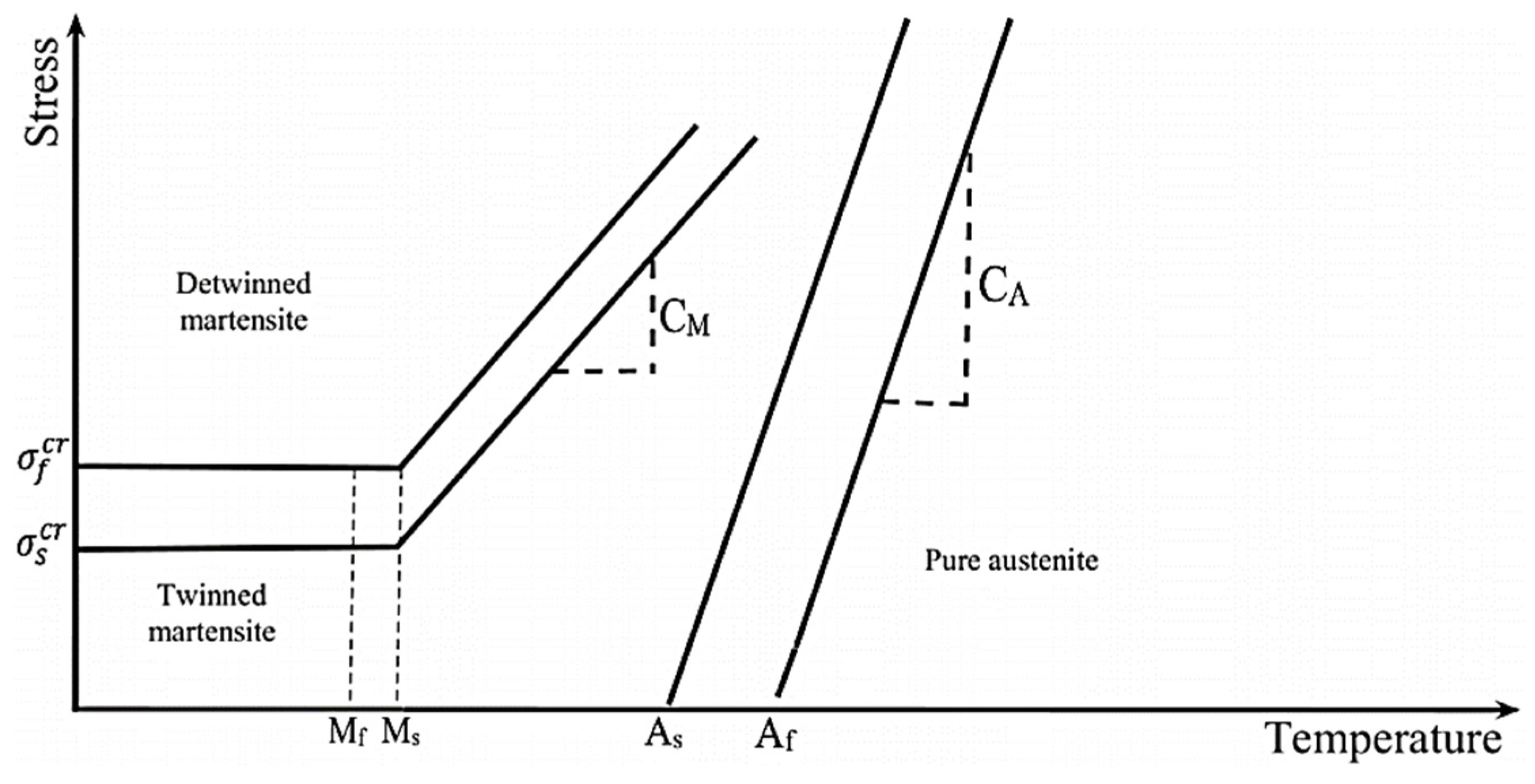
where E_M stands for the elastic modulus in the martensite phase, and E_A corresponds to the austenite phase. The phase transformation is initiated at specific temperatures, known as M_s (martensite start), A_s (austenite start), M_f (martensite finish), and A_f (austenite finish) temperatures under zero-stress conditions. The stresses associated with the detwinning start and finish processes are symbolized as ${\sigma }_s^{cr}$ and ${\sigma }_f^{cr}$, respectively. C_M signifies the constant that illustrates the influence of stress coefficients, and C_A (as depicted in Figure 4) represents the impact of stress on the transformation temperatures of the martensite and austenite phases [30].

To determine the martensitic fractions concerning both temperature and stress (as depicted in Figure 4), the progression of equations can be delineated as follows:

For $T>M_S$ and ${\sigma }_s^{cr}+C_M\left(T-M_S\right)<\sigma <{\sigma }_f^{cr}+C_M\left(T-M_S\right)$,

$${\xi }_S=\frac{1-{\xi }_{50}}{2}\mathrm{c}\mathrm{o}\mathrm{s} \left\{\frac{\pi }{{\sigma }_S^{cr}-{\sigma }_f^{cr}}\left[\sigma -{\sigma }_f^{cr}-C_M\left(T-M_S\right)\right\}+\frac{1+{\xi }_{s0}}{2}\right.,$$

$${\xi }_T={\xi }_{T0}-\frac{{\xi }_{T0}}{1-{\xi }_{S0}}\left({\xi }_s-{\xi }_{s0}\right).$$

(38)

Also, for $T<M_S$ and ${\sigma }_s^{cr}<\sigma <{\sigma }_f^{cr}$,

$${\xi }_S=\frac{1-{\xi }_{S0}}{2}\mathrm{c}\mathrm{o}\mathrm{s} \left\{\frac{\pi }{{\sigma }_S^{cr}-{\sigma }_f^{cr}}\left(\sigma -{\sigma }_f^{cr}\right)\right\}+\frac{1+{\xi }_{s0}}{2},$$

$${\xi }_T={\xi }_{T0}-\frac{{\xi }_{T0}}{1-{\xi }_{s0}}\left({\xi }_s-{\xi }_{s0}\right)+{\mathsf{\Delta }}_{T\epsilon }.$$

(39)

where, if $M_f<T<M_S$ and $T<T_0,$

$${\mathsf{\Delta }}_{T\epsilon }=\frac{1-{\xi }_{T0}}{2}\left\{\mathrm{c}\mathrm{o}\mathrm{s} \left[a_M\left(T-M_f\right)\right]+1\right\},$$

(40)

else ${\mathsf{\Delta }}_{T\epsilon }=0$.

For $T>A_S$ and $C_A\left(T-A_f\right)<\sigma <C_A\left(T-A_S\right)$,

$$\begin{array}{c}\xi =\frac{{\xi }_0}{2}\left\{\mathrm{c}\mathrm{o}\mathrm{s} \left[a_A\left(T-A_S-\frac{\sigma }{C_A}\right)\right]+1\right\}\hfill \\ {\xi }_s={\xi }_{s0}-\frac{{\xi }_{s0}}{{\xi }_0}\left({\xi }_0-\xi \right)\hfill \\ {\xi }_T={\xi }_{T0}-\frac{{\xi }_{T0}}{{\xi }_0}\left({\xi }_0-\xi \right)\hfill \end{array}.$$

(41)

Here, the parameters (T₀, ξ S₀, ξ T₀, and ξ₀) denote the initial state of the material. Additionally, $a_A$ and $a_M$ are material constants defined as:

$$a_A=\frac{\pi }{A_f-A_s},$$

(42)

$$a_M=\frac{\pi }{M_s-M_f}.$$

(43)

The behavior of the shape memory alloy is characterized by a nonlinear function involving temperature, stress, and pressure, which are considered to be independent and unrelated to each other [32].

Moreover, concerning the mathematical techniques and models within the framework of SMA (shape memory alloy), the fundamental framework of the model was elucidated through the utilization of a rheological model [33]. The foundational kinematic assumptions of the finite deformation model and the Helmholtz free energy function were detailed [34], and the exploitation of the Clausius–Duhem inequality was employed to derive the constitutive inequalities [33]. These inequalities serve as the basis for establishing the evolution equations.

3.4. Constitutive Models

3.4.1. Linear Elastic Constitutive Model

The linear elastic constitutive model, deeply rooted in Hooke’s Law, a fundamental principle in mechanics, has had a profound impact on various fields of science and engineering. This model establishes a proportional relationship between the strain (change in shape or size) in a material and the applied stress (force) within the elastic limit of that material [35]. This linear relationship forms the cornerstone of understanding material behavior, and it has proven to be invaluable in the context of ankle–foot orthosis (AFO) design. To understand the significance of the linear elastic constitutive model, we must first trace its origins to Hooke’s Law, a cornerstone principle in mechanics [36]. In mathematical terms, this relationship is expressed as:

$$\sigma =Eϵ.$$

(44)

In this equation, $\sigma$ represents the stress applied to the material, $E$ stands for the material’s Young’s modulus (a constant that characterizes the material’s stiffness), and $ϵ$ denotes the strain.

This fundamental law is a precursor to the linear elastic constitutive model and serves as its conceptual foundation [37]. Hooke’s Law established the initial understanding that the response of a material to an applied force is linear within the elastic limit, and this notion is encapsulated in the linear elastic constitutive model.

The linear elastic constitutive model is often presented in terms of tensorial quantities, particularly emphasizing the fourth-order elasticity or stiffness tensor. This tensor is a comprehensive mathematical framework that describes the relationship between stress and strain in a material. The generalized Hooke’s Law, which encapsulates this relationship, defines a linear relation among all the components of the stress and strain tensor and is represented as [35]:

$${\sigma }_{ij}=C_{ijkl}{ϵ}_{kl}.$$

(45)

In this equation, ${\sigma }_{ij}$ represents the components of the stress tensor, ${ϵ}_{kl}$ denotes the components of the strain tensor, and $C_{ijkl}$signifies the components of the fourth-order stiffness tensor. For a three-dimensional context, this tensor comprises a total of 81 components, while two-dimensional problems reduce the count to 16 components. The inclusion of tensorial quantities in this model underscores its versatility and applicability to a wide range of materials and structures. This tensor-based approach is capable of describing complex mechanical behaviors and allows for the modeling of materials with varying properties in different directions. This mathematical framework is particularly well-suited for materials with anisotropic properties, where stiffness and elasticity differ along different axes [38,39].

The utility of the linear elastic constitutive model extends far beyond theoretical considerations. This model has found widespread use in the field of biomechanics, where understanding the mechanical properties of human tissues, as well as the design and analysis of orthotic devices like AFOs is of paramount importance. Researchers have harnessed this model to gain deeper insights into the behavior of human tissues, particularly in the context of AFO design. For example, studies have employed finite element analysis, a computational technique for solving complex problems, to investigate the three-dimensional behavior of the human foot during activities like standing. These studies have employed the linear elastic constitutive model to describe the mechanical properties of the foot tissues, offering valuable insights into the stresses and strains experienced by the foot under various conditions [37].

Similarly, computational models have been developed to study the effect of foot constraint on ankle injuries. These models incorporate the linear elastic constitutive model to represent the mechanical behavior of the ligaments and foot structures, providing a deeper understanding of how these structures respond to various loads and constraints [40]. Moreover, the linear elastic constitutive model has been instrumental in the design and optimization of AFOs. Researchers and engineers have utilized this model in virtual prototyping processes for the manufacture of passive–dynamic AFOs [41]. By simulating the bending stiffness of the orthotic device, they can optimize its design for improved performance and patient comfort. This process has accelerated the development and refinement of AFOs, leading to more effective orthotic devices [42].

One of the most significant contributions of the linear elastic constitutive model to AFO design is the ability to customize orthotic devices to cater to the unique biomechanical needs of individual patients. This is especially critical in the field of orthotics and rehabilitation, where every patient’s condition and requirements are distinct [43]. The model’s versatility is apparent in its influence on material selection for AFOs. The choice of materials is a fundamental aspect of orthotic design, as it directly impacts the device’s performance. The linear elastic constitutive model offers orthotists a starting point for material selection. Stiffer materials, as guided by the model, are preferred when the goal is to enhance support and stability in AFOs. These materials are well-suited for patients requiring significant structural support or conditions requiring rigid bracing [44].

Conversely, more flexible materials are advantageous when the objective is controlled deformation, allowing for the mimicry of natural foot movement [45]. These materials are particularly useful in cases where patients need a more dynamic and accommodating orthotic device. The model empowers orthotists to tailor AFOs to the specific biomechanical needs of individual patients, ensuring an optimal balance between support and comfort. This customization is vital for enhancing patient compliance and overall quality of life [46]. The ability to select and customize materials based on the linear elastic constitutive model offers orthotists a systematic and science-based approach to AFO design. This approach ensures that the materials used are not only appropriate for the intended purpose but also contribute to the overall effectiveness of the orthotic device.

The linear elastic constitutive model offers several distinct advantages that have made it a vital tool in the field of AFO design and biomechanics [47]: (1) simplicity—The model’s linear approach is straightforward and relatively easy to understand, providing a clear foundation for analyzing material behavior within the elastic limit; (2) predictability—the model’s linear nature allows for predictable and repeatable results, making it a reliable tool for engineers and orthotists; (3) versatility—the inclusion of tensorial quantities in the model enables it to describe a wide range of materials, including anisotropic materials with varying properties along different axes; (4) customization—the model empowers orthotists to tailor AFOs to individual patient’s needs, balancing support and comfort effectively; (5) accelerated development—the use of this model in virtual prototyping processes has accelerated the development and refinement of AFOs, leading to more effective orthotic devices.

However, like any model, the linear elastic constitutive model has its limitations [48,49]: (1) linear elastic assumption—the model simplifies material behavior to linear elasticity. In reality, many materials exhibit nonlinear behavior under certain conditions, such as plastic deformation or material failure. The model cannot accurately represent such phenomena; (2) real-world complexities—designers and orthotists must use this model judiciously, considering the specific properties of materials and the real-world conditions to which AFOs will be subjected. In practice, materials often exhibit complex behaviors beyond the scope of linear elasticity; (3) limited to elastic range—the model is applicable only within the elastic limit of materials. Beyond this limit, materials may exhibit irreversible deformations and complex behavior that cannot be accurately predicted by the linear model.

In practice, it is essential to acknowledge these limitations and apply the model within its appropriate scope. Orthotists and engineers should use the model as a foundational tool but be prepared to account for nonlinear behaviors and other complexities when designing and manufacturing AFOs for real-world applications [50].

3.4.2. Viscoelastic Constitutive Model

Viscoelasticity is a fascinating property observed in materials that exhibit both viscous and elastic characteristics when subjected to deformation. This unique behavior, where materials display both time-dependent strain and stress responses, has significant relevance in various fields [51], including material science, engineering, and particularly in the construction of ankle–foot orthoses (AFOs) [52]. The viscoelastic constitutive model, a mathematical model designed to characterize and predict the mechanical behavior of viscoelastic materials, plays a pivotal role in understanding and utilizing these materials effectively [53].

The mechanical behavior of viscoelastic materials is inherently complex due to its time-dependent nature [54]. To accurately capture this behavior, the viscoelastic constitutive model employs intricate mathematical representations. One common form of this equation can be expressed as:

$$\sigma (t)={\int }_0^t G(t-\tau )\frac{dϵ\left(\tau \right)}{d\tau }d\tau .$$

(46)

In this equation, $\sigma \left(t\right)$ represents the stress at time $t$, $ϵ\left(\tau \right)$ denotes the strain at time $\tau$, and $G(t-\tau )$ is a relaxation function that describes how the material response changes over time. This equation captures the complex interplay between stress and strain in viscoelastic materials and has a direct application in the design of AFOs.

Viscoelastic materials exhibit several distinctive characteristics that set them apart from purely elastic materials. Understanding these properties is fundamental to comprehending the behavior of these materials in real-world applications: (1) hysteresis—viscoelastic materials exhibit hysteresis, a fundamental property characterized by the energy dissipation within the material during loading and unloading cycles. This behavior underscores the role of viscous properties in dissipating energy, a critical aspect of viscoelasticity [55]; (2) creep—creep is another defining characteristic of viscoelastic materials. It refers to the increase in strain under constant stress over time. This phenomenon is often observed in materials used in AFOs, reflecting the materials’ tendency to deform under prolonged stress, making it particularly relevant in orthotic design; (3) stress relaxation—stress relaxation represents the decrease in stress under constant strain over time, illustrating the material’s ability to adapt its response to changing conditions. This property is crucial in AFO design, as orthotic devices must provide support while accommodating changes in stress over time, especially during activities like walking [56].

The viscoelastic constitutive model, while offering a more accurate description of material behavior, introduces increased complexity to the analysis. The time-dependent nature of the material response necessitates the use of more advanced numerical methods for solving problems involving viscoelastic materials. This complexity can involve intricate differential equations, numerical integration techniques, and a deeper understanding of the underlying material properties [57].

The unique properties of viscoelastic materials have a direct application in the design and optimization of AFOs, which must accommodate the dynamic and varied loads experienced during activities such as gait, all while ensuring patient comfort and support. By applying the viscoelastic constitutive model, orthotists and engineers can predict how viscoelastic materials will deform and respond to diverse loading conditions. This approach allows for the creation of more effective AFOs tailored to individual patient needs, optimizing the balance between support and comfort [58].

Furthermore, the understanding of viscoelastic material behavior enables AFO designers to consider time-dependent effects in orthotic design, enhancing the overall performance of these devices. It ensures that AFOs are not solely designed based on the assumption of linear elasticity, which is a simplification often used for purely elastic materials. By accounting for viscoelasticity, orthotic devices can more accurately mimic natural biomechanics, providing patients with a higher level of comfort and functionality during daily activities.

3.4.3. Hyperelastic Constitutive Model

Hyperelastic constitutive models, often referred to as strain energy density functions or material models, are fundamental tools in the field of biomechanics [59] and material science [60]. These models, rooted in the theory of elasticity, provide a systematic approach to characterize the behavior of materials, particularly those used in ankle–foot orthoses (AFO). Hyperelastic models are especially valued for their ability to capture the nonlinear, time-independent response of materials to deformation. One of the most recognized hyperelastic models is the neo-Hookean model, exemplifying the essence of these equations [53].

At the heart of the hyperelastic constitutive model lies the mathematical representation that characterizes the material behavior [61]. This representation hinges on the definition of a strain energy density function, $W$, in terms of the deformation gradient, $F$. The neo-Hookean model, an archetype of hyperelastic models, can be expressed as [62]:

$$W=\frac{\mu }{2}\left(I_1-3\right)-\mu \mathrm{l}\mathrm{n} (J)+\frac{\lambda }{2}{\mathrm{l}\mathrm{n}}^2 (J).$$

(47)

Here, $W$ symbolizes the strain energy density function, while $\mu$ and $\lambda$ are material constants. $I_1$ represents the first invariant of the deformation tensor, and $J$ denotes the determinant of the deformation gradient. The neo-Hookean model captures the essential characteristics of hyperelastic materials, providing a foundation for understanding their complex behavior [63].

The hyperelastic constitutive model plays a pivotal role in AFO design. AFOs must accommodate the dynamic and varied loads experienced during gait while ensuring patient comfort and support [64]. The application of hyperelastic models enables orthotists and engineers to predict the deformation of materials under diverse loading conditions, thereby ensuring AFOs deliver the requisite support and flexibility to patients with a wide spectrum of pathologies [65].

The hyperelastic constitutive model offers several advantages in the realm of AFO design [66], including: (1) nonlinearity—these models capture the nonlinear behavior of materials, providing a more accurate representation of the intricate deformations occurring in AFOs; (2) customization—orthotists can tailor AFO designs by adjusting material parameters, and matching the orthotic device to the specific biomechanical needs of individual patients; (3) predictive modeling—the models allow orthotists and designers to predict material responses under various loading conditions, facilitating the creation of more effective and patient-specific AFOs. Despite their advantages, the hyperelastic constitutive model is not without limitations [67]. These include: (1) material complexity—not all materials can be accurately described by a single hyperelastic model. More complex materials may require the incorporation of multi-physics models to account for their unique characteristics; (2) parameter estimation—accurately determining material parameters for hyperelastic models can be a challenging endeavor, often requiring extensive experimentation and testing.

The hyperelastic constitutive model, with the neo-Hookean model as a prominent example, plays a crucial role in AFO design [68]. Their ability to accurately capture nonlinear material behavior, enable customization, and support predictive modeling makes them indispensable tools in the creation of orthotic devices that enhance patient mobility, comfort, and overall quality of life. The broader implications of these models extend into material science, biomechanics, and personalized healthcare, where the principles of hyperelasticity continue to shape how we understand and manipulate the physical world [69].

4. Conclusions

In summary, this review of the literature on mathematical methods applications in the biomechanics of foot and ankle–foot orthosis models has uncovered several crucial insights, shaping the future of this field. Regarding the nonlinear optimization and Cartesian coordinates, it is found that employing nonlinear optimization in fully Cartesian coordinates enhances our understanding of AFOs’ kinematic and dynamic aspects. This opens avenues for more advanced and effective AFO designs. In terms of robotic rehabilitation with two-degree-of-freedom AFO, the exploration of a two-degree-of-freedom AFO for robotic rehabilitation stands out as a promising approach. Considering the interplay between foot and orthosis models, this innovation has the potential to significantly impact rehabilitation strategies. Regarding the shape memory alloy (SMA) elements in AFOs, the review underscores the growing trend of incorporating shape memory alloy (SMA) elements in AFOs. This suggests exciting possibilities for further research and development, offering potential benefits in AFO functionality. Additionally, the diversity of constitutive models, including linear elastic, viscoelastic, and hyperelastic models, emerged as a key finding. Understanding these models is crucial for tailoring AFO designs to individual patient needs, providing a more personalized approach to orthotic interventions.

Building on these insights, future research in AFOs should prioritize: (1) innovative mathematical models—explore new mathematical models and optimization techniques to enhance precision in AFO design; (2) clinical implications of novel designs—investigate the long-term clinical implications and patient outcomes associated with innovative AFO designs, especially those incorporating SMA elements; (3) interdisciplinary collaboration—encourage collaboration between orthotists, engineers, and clinicians to bridge the gap between theoretical advancements and practical applications in patient care.

References

- Daryabor, A.; Arazpour, M.; Aminian, G.; Baniasad, M.; Yamamoto, S. Design and Evaluation of an Articulated Ankle Foot Orthosis with Plantarflexion Resistance on the Gait: A Case Series of 2 Patients with Hemiplegia. J. Biomed. Phys. Eng. 2020, 10, 119–120. [Google Scholar] [CrossRef] [PubMed]
- Nazha, H.M.; Szávai, S.; Darwich, M.A.; Juhre, D. Passive Articulated and Non-Articulated Ankle-Foot Orthoses for Gait Rehabilitation: A Narrative Review. Healthcare 2023, 11, 947. [Google Scholar] [CrossRef] [PubMed]
- Breitman, N.; Yona, T.; Fischer, A.G. Gait Event Detection Wearable Device Development and the Effect of Vibration Feedback on Ankle Kinematics and Kinetics. IEEE Sens. J. 2023, 23, 19052–19059. [Google Scholar] [CrossRef]
- Darwich, A.; Nazha, H.; Sliman, A.; Abbas, W. Ankle-Foot Orthosis Design between the Tradition and the Computerized Perspectives. Int. J. Artif. Organs 2020, 43, 354–361. [Google Scholar] [CrossRef] [PubMed]
- Tan, B.H.M.; Nather, A.; David, V. Biomechanics of the Foot. In Diabetic Foot Problems; World Scientific: Singapore, 2008; pp. 67–75. ISBN 9789812791511. [Google Scholar]
- Zajac, F.E.; Neptune, R.R.; Kautz, S.A. Biomechanics and Muscle Coordination of Human Walking: Part II: Lessons from Dynamical Simulations and Clinical Implications. Gait Posture 2003, 17, 1–17. [Google Scholar] [CrossRef] [PubMed]
- Raja, B.; Neptune, R.R.; Kautz, S.A. Quantifiable Patterns of Limb Loading and Unloading during Hemiparetic Gait: Relation to Kinetic and Kinematic Parameters. J. Rehabil. Res. Dev. 2012, 49, 1293–1304. [Google Scholar] [CrossRef] [PubMed]
- Otten, E. Inverse and Forward Dynamics: Models of Multi-Body Systems. Philos. Trans. R. Soc. Lond. B Biol. Sci. 2003, 358, 1493–1500. [Google Scholar] [CrossRef] [PubMed]
- Cleather, D.J.; Bull, A.M.J. Influence of Inverse Dynamics Methods on the Calculation of Inter-Segmental Moments in Vertical Jumping and Weightlifting. Biomed. Eng. Online 2010, 9, 74. [Google Scholar] [CrossRef]
- Karatsidis, A.; Bellusci, G.; Schepers, H.M.; de Zee, M.; Andersen, M.S.; Veltink, P.H. Estimation of Ground Reaction Forces and Moments during Gait Using Only Inertial Motion Capture. Sensors 2016, 17, 75. [Google Scholar] [CrossRef]
- Buchanan, T.S.; Lloyd, D.G.; Manal, K.; Besier, T.F. Neuromusculoskeletal Modeling: Estimation of Muscle Forces and Joint Moments and Movements from Measurements of Neural Command. J. Appl. Biomech. 2004, 20, 367–395. [Google Scholar] [CrossRef]
- Lugrís, U.; Carlín, J.; Pàmies-Vilà, R.; Font-Llagunes, J.M.; Cuadrado, J. Solution Methods for the Double-Support Indeterminacy in Human Gait. Multibody Syst. Dyn. 2013, 30, 247–263. [Google Scholar] [CrossRef]
- Liu, L.; Cooper, J.L.; Ballard, D.H. Computational Modeling: Human Dynamic Model. Front. Neurorobot. 2021, 15, 723428. [Google Scholar] [CrossRef] [PubMed]
- Isler, K.; Payne, R.C.; Günther, M.M.; Thorpe, S.K.S.; Li, Y.; Savage, R.; Crompton, R.H. Inertial Properties of Hominoid Limb Segments. J. Anat. 2006, 209, 201–218. [Google Scholar] [CrossRef] [PubMed]
- Ambrósio, J.A.C.; Kecskeméthy, A. Multibody Dynamics of Biomechanical Models for Human Motion via Optimization. In Computational Methods in Applied Sciences; Springer Netherlands: Dordrecht, The Netherlands, 2007; pp. 245–272. ISBN 9781402056833. [Google Scholar]
- Neves, M.C. Design of Ankle Foot Orthoses Using Subject Specific Biomechanical Data and Optimization Tools. Master’s Thesis, Instituto Superior Técnico, Universidade de Lisboa, Lisboa, Portugal, 2014. [Google Scholar]
- Ruggiero, A.; Sicilia, A. A Novel Explicit Analytical Multibody Approach for the Analysis of Upper Limb Dynamics and Joint Reactions Calculation Considering Muscle Wrapping. Appl. Sci. 2020, 10, 7760. [Google Scholar] [CrossRef]
- Welch, E.B.; Manduca, A.; Grimm, R.C.; Ward, H.A.; Jack, C.R., Jr. Spherical Navigator Echoes for Full 3D Rigid Body Motion Measurement in MRI. Magn. Reson. Med. 2002, 47, 32–41. [Google Scholar] [CrossRef]
- Milica, L.; Năstase, A.; Andrei, G. A Novel Algorithm for the Absorbed Power Estimation of HEXA Parallel Mechanism Using an Extended Inverse Dynamic Model. Proc. Inst. Mech. Eng. K J. Multi-body Dyn. 2020, 234, 185–197. [Google Scholar] [CrossRef]
- Sellers, W.I.; Crompton, R.H. A System for 2-and 3D Kinematic and Kinetic Analysis of Locomotion, and Its Application to Analysis of the Energetic Efficiency of Jumping Locomotion. Z. Morphol. Anthropol. 1994, 80, 99–108. Available online: https://www.jstor.org/stable/25757420 (accessed on 10 October 2023). [CrossRef]
- Wojtyra, M.; Frączek, J. Solvability of Reactions in Rigid Multibody Systems with Redundant Nonholonomic Constraints. Multibody Syst. Dyn. 2013, 30, 153–171. [Google Scholar] [CrossRef]
- Vilà, R.P. Application of Multibody Dynamics Techniques to the Analysis of Human Gait. Ph.D. Thesis, Universitat Politècnica de Catalunya, Barcelona, Spain, 2012. [Google Scholar]
- Erdemir, A.; McLean, S.; Herzog, W.; van den Bogert, A.J. Model-Based Estimation of Muscle Forces Exerted during Movements. Clin. Biomech. 2007, 22, 131–154. [Google Scholar] [CrossRef]
- Patar, A.; Jamlus, N.; Makhtar, K.; Mahmud, J.; Komeda, T. Development of Dynamic Ankle Foot Orthosis for Therapeutic Application. Procedia Eng. 2012, 41, 1432–1440. [Google Scholar] [CrossRef]
- Agrawal, A.; Sangwan, V.; Banala, S.K.; Agrawal, S.K.; Binder-Macleod, S.A. Design of a Novel Two Degree-of-Freedom Ankle-Foot Orthosis. J. Mech. Des. N. Y. 2007, 129, 1137–1143. [Google Scholar] [CrossRef]
- Darwich, A.; Nazha, H.; Nazha, A.; Daoud, M.; Alhussein, A. Bio-Numerical Analysis of the Human Ankle-Foot Model Corresponding to Neutral Standing Condition. J. Biomed. Phys. Eng. 2020, 10, 645–650. [Google Scholar] [CrossRef] [PubMed]
- Nordin, M.; Frankel, V.H. Basic Biomechanics of the Musculoskeletal System; Lippincott Williams & Wilkins: Philadelphia, PA, USA, 2001. [Google Scholar]
- Gosselin, C.M. Fundamentals of Robotic Mechanical Systems: Theory, Methods, and Algorithms, Jorge Angeles, Springer, New York, NY, 1997. ISBN 0-387-94540-7. Int. J. Robust Nonlinear Control 2000, 10, 1359. [Google Scholar] [CrossRef]
- Poorasadion, S.; Arghavani, J.; Naghdabadi, R.; Sohrabpour, S. An Improvement on the Brinson Model for Shape Memory Alloys with Application to Two-Dimensional Beam Element. J. Intell. Mater. Syst. Struct. 2014, 25, 1905–1920. [Google Scholar] [CrossRef]
- Brinson, L.C.; Huang, M.S. Simplifications and Comparisons of Shape Memory Alloy Constitutive Models. J. Intell. Mater. Syst. Struct. 1996, 7, 108–114. [Google Scholar] [CrossRef]
- Sayyaadi, H.; Zakerzadeh, M.R.; Salehi, H. A Comparative Analysis of Some One-Dimensional Shape Memory Alloy Constitutive Models Based on Experimental Tests. Sci. Iran. 2012, 19, 249–257. [Google Scholar] [CrossRef]
- Sadeghian, F.; Zakerzadeh, M.R.; Karimpour, M.; Baghani, M. Numerical Study of Patient-Specific Ankle-Foot Orthoses for Drop Foot Patients Using Shape Memory Alloy. Med. Eng. Phys. 2019, 69, 123–133. [Google Scholar] [CrossRef]
- Reese, S.; Christ, D. Finite Deformation Pseudo-Elasticity of Shape Memory Alloys-Constitutive Modelling and Finite Element Implementation. Int. J. Plast. 2008, 24, 455–482. [Google Scholar] [CrossRef]
- Christ, D.; Reese, S. A Finite Element Model for Shape Memory Alloys Considering Thermomechanical Couplings at Large Strains. Int. J. Solids Struct. 2009, 46, 3694–3709. [Google Scholar] [CrossRef]
- Mase, G.T.; Smelser, R.E.; Mase, G.E. Continuum Mechanics for Engineers, 3rd ed.; CRC Press: Boca Raton, FL, USA, 2009; ISBN 9780429139284. [Google Scholar]
- Zhou, X.-P.; Tian, D.-L. A Novel Linear Elastic Constitutive Model for Continuum-Kinematics-Inspired Peridynamics. Comput. Methods Appl. Mech. Eng. 2021, 373, 113479. [Google Scholar] [CrossRef]
- Cheung, J.T.-M.; Zhang, M.; Leung, A.K.-L.; Fan, Y.-B. Three-Dimensional Finite Element Analysis of the Foot during Standing—A Material Sensitivity Study. J. Biomech. 2005, 38, 1045–1054. [Google Scholar] [CrossRef] [PubMed]
- Zhou, X.; Wang, Y.; Shou, Y.; Kou, M. A Novel Conjugated Bond Linear Elastic Model in Bond-Based Peridynamics for Fracture Problems under Dynamic Loads. Eng. Fract. Mech. 2018, 188, 151–183. [Google Scholar] [CrossRef]
- Weeger, O. Numerical Homogenization of Second Gradient, Linear Elastic Constitutive Models for Cubic 3D Beam-Lattice Metamaterials. Int. J. Solids Struct. 2021, 224, 111037. [Google Scholar] [CrossRef]
- Wei, F.; Hunley, S.C.; Powell, J.W.; Haut, R.C. Development and Validation of a Computational Model to Study the Effect of Foot Constraint on Ankle Injury Due to External Rotation. Ann. Biomed. Eng. 2011, 39, 756–765. [Google Scholar] [CrossRef] [PubMed]
- Schrank, E.S.; Hitch, L.; Wallace, K.; Moore, R.; Stanhope, S.J. Assessment of a Virtual Functional Prototyping Process for the Rapid Manufacture of Passive-Dynamic Ankle-Foot Orthoses. J. Biomech. Eng. 2013, 135, 101011. [Google Scholar] [CrossRef] [PubMed]
- Faustini, M.C.; Neptune, R.R.; Crawford, R.H.; Stanhope, S.J. Manufacture of Passive Dynamic Ankle-Foot Orthoses Using Selective Laser Sintering. IEEE Trans. Biomed. Eng. 2008, 55, 784–790. [Google Scholar] [CrossRef] [PubMed]
- Tyson, S.F.; Kent, R.M. Effects of an Ankle-Foot Orthosis on Balance and Walking after Stroke: A Systematic Review and Pooled Meta-Analysis. Arch. Phys. Med. Rehabil. 2013, 94, 1377–1385. [Google Scholar] [CrossRef] [PubMed]
- Kerkum, Y.L.; Buizer, A.I.; van den Noort, J.C.; Becher, J.G.; Harlaar, J.; Brehm, M.-A. The Effects of Varying Ankle Foot Orthosis Stiffness on Gait in Children with Spastic Cerebral Palsy Who Walk with Excessive Knee Flexion. PLoS ONE 2015, 10, e0142878. [Google Scholar] [CrossRef]
- Wojciechowski, E.; Chang, A.Y.; Balassone, D.; Ford, J.; Cheng, T.L.; Little, D.; Menezes, M.P.; Hogan, S.; Burns, J. Feasibility of Designing, Manufacturing and Delivering 3D Printed Ankle-Foot Orthoses: A Systematic Review. J. Foot Ankle Res. 2019, 12, 11. [Google Scholar] [CrossRef]
- Ries, A.J.; Novacheck, T.F.; Schwartz, M.H. The Efficacy of Ankle-foot Orthoses on Improving the Gait of Children with Diplegic Cerebral Palsy: A Multiple Outcome Analysis. PM R 2015, 7, 922–929. [Google Scholar] [CrossRef]
- Mavroidis, C.; Ranky, R.G.; Sivak, M.L.; Patritti, B.L.; DiPisa, J.; Caddle, A.; Gilhooly, K.; Govoni, L.; Sivak, S.; Lancia, M.; et al. Patient Specific Ankle-Foot Orthoses Using Rapid Prototyping. J. Neuroeng. Rehabil. 2011, 8, 1. [Google Scholar] [CrossRef] [PubMed]
- Athanasiou, K.; Natoli, R. Introduction to Continuum Biomechanics; Springer Nature: Berlin/Heidelberg, Germany, 2022; ISBN 978-3-031-00498-8. [Google Scholar] [CrossRef]
- Yeung, L.-F.; Ockenfeld, C.; Pang, M.-K.; Wai, H.-W.; Soo, O.-Y.; Li, S.-W.; Tong, K.-Y. Randomized Controlled Trial of Robot-Assisted Gait Training with Dorsiflexion Assistance on Chronic Stroke Patients Wearing Ankle-Foot-Orthosis. J. Neuroeng. Rehabil. 2018, 15, 51. [Google Scholar] [CrossRef] [PubMed]
- Chen, R.K.; Jin, Y.-A.; Wensman, J.; Shih, A. Additive Manufacturing of Custom Orthoses and Prostheses—A Review. Addit. Manuf. 2016, 12, 77–89. [Google Scholar] [CrossRef]
- Fung, Y.C.; Cowin, S.C. Biomechanics: Mechanical Properties of Living Tissues, 2nd Ed. J. Appl. Mech. 1994, 61, 1007. [Google Scholar] [CrossRef]
- Allen, D.P.; Little, R.; Laube, J.; Warren, J.; Voit, W.; Gregg, R.D. Towards an Ankle-Foot Orthosis Powered by a Dielectric Elastomer Actuator. Mechatronics 2021, 76, 102551. [Google Scholar] [CrossRef]
- Mow, V.C.; Huiskes, R. Basic Orthopaedic Biomechanics & Mechano-Biology; Lippincott Williams & Wilkins: Philadelphia, PA, USA, 2005; ISBN 0-7817-3933-0. [Google Scholar]
- Afoke, N.Y.; Hunt, N.P. Viscoelasticity in Dentistry: A Review. J. Dent. 1996, 24, 307–313. [Google Scholar]
- Sharma, S.; Shankar, V.; Joshi, Y.M. Viscoelasticity and Rheological Hysteresis. J. Rheol. 2023, 67, 139–155. [Google Scholar] [CrossRef]
- Lin, C.-Y.; Chen, Y.-C.; Lin, C.-H.; Chang, K.-V. Constitutive Equations for Analyzing Stress Relaxation and Creep of Viscoelastic Materials Based on Standard Linear Solid Model Derived with Finite Loading Rate. Polymers 2022, 14, 2124. [Google Scholar] [CrossRef]
- Holmes, M.H.; Lai, W.M. Viscoelastic Properties of Arteries: Segmental Behavior and Mechanical Anisotropy. J. Biomech. 1992, 25, 35–41. [Google Scholar]
- Sacks, M.S. Incorporation of Experimentally-Derived Fiber Orientation into a Structural Constitutive Model for Planar Collagenous Tissues. J. Biomech. Eng. 2003, 125, 280–287. [Google Scholar] [CrossRef]
- Khaniki, H.B.; Ghayesh, M.H.; Chin, R.; Amabili, M. Hyperelastic Structures: A Review on the Mechanics and Biomechanics. Int. J. Non Linear Mech. 2023, 148, 104275. [Google Scholar] [CrossRef]
- Mihai, L.A.; Goriely, A. How to Characterize a Nonlinear Elastic Material? A Review on Nonlinear Constitutive Parameters in Isotropic Finite Elasticity. Proc. Math. Phys. Eng. Sci. 2017, 473, 20170607. [Google Scholar] [CrossRef] [PubMed]
- Xiangfeng, P.; Luxian, L. State of the Art of Constitutive Relations of Hyperelastic Materials. Chin. J. Theor. Appl. Mech. 2020, 52, 1221–1232. [Google Scholar] [CrossRef]
- Chagnon, G.; Rebouah, M.; Favier, D. Hyperelastic Energy Densities for Soft Biological Tissues: A Review. J. Elast. 2015, 120, 129–160. [Google Scholar] [CrossRef]
- Zhan, L.; Wang, S.; Qu, S.; Steinmann, P.; Xiao, R. A New Micro–Macro Transition for Hyperelastic Materials. J. Mech. Phys. Solids 2023, 171, 105156. [Google Scholar] [CrossRef]
- Emminger, C.; Çakmak, U.D.; Preuer, R.; Graz, I.; Major, Z. Hyperelastic Material Parameter Determination and Numerical Study of TPU and PDMS Dampers. Materials 2021, 14, 7639. [Google Scholar] [CrossRef] [PubMed]
- Ramzanpour, M.; Hosseini-Farid, M.; McLean, J.; Ziejewski, M.; Karami, G. Visco-Hyperelastic Characterization of Human Brain White Matter Micro-Level Constituents in Different Strain Rates. Med. Biol. Eng. Comput. 2020, 58, 2107–2118. [Google Scholar] [CrossRef]
- Hashiguchi, K. Multiplicative Hyperelastic-Based Plasticity for Finite Elastoplastic Deformation/Sliding: A Comprehensive Review. Arch. Comput. Methods Eng. 2019, 26, 597–637. [Google Scholar] [CrossRef]
- Gasser, T.C.; Ogden, R.W.; Holzapfel, G.A. Hyperelastic Modelling of Arterial Layers with Distributed Collagen Fibre Orientations. J. R. Soc. Interface 2006, 3, 15–35. [Google Scholar] [CrossRef]
- Ielapi, A.; Lammens, N.; Van Paepegem, W.; Forward, M.; Deckers, J.P.; Vermandel, M.; De Beule, M. A Validated Computational Framework to Evaluate the Stiffness of 3D Printed Ankle Foot Orthoses. Comput. Methods Biomech. Biomed. Engin. 2019, 22, 880–887. [Google Scholar] [CrossRef]
- Marckmann, G.; Verron, E. Comparison of Hyperelastic Models for Rubber-like Materials. Rubber Chem. Technol. 2006, 79, 835–858. [Google Scholar] [CrossRef]
Figure 1.
Selection of studies based on the PRISMA flow diagram.
Figure 2.
Illustration of the orientations of the plantarflexion–dorsiflexion joint axis () and the eversion–inversion joint axis (), along with their corresponding kinematic representations [25], with permission from the American Society of Mechanical Engineers ASME (License Number: 1408140-1).
Figure 3.
Machine and human parts of the shank and ankle [25], with permission from the American Society of Mechanical Engineers ASME (License Number: 1408141-1).
Figure 4.
The essential stress–temperature profiles pertaining to the Brinson model’s critical behavior [31], with permission from Elsevier (Creative Commons license, https://creativecommons.org/licenses/by-nc-nd/4.0/ (accessed on 15 October 2023)).
Disclaimer/Publisher’s Note: The statements, opinions and data contained in all publications are solely those of the individual author(s) and contributor(s) and not of MDPI and/or the editor(s). MDPI and/or the editor(s) disclaim responsibility for any injury to people or property resulting from any ideas, methods, instructions or products referred to in the content. |
© 2023 by the authors. Licensee MDPI, Basel, Switzerland. This article is an open access article distributed under the terms and conditions of the Creative Commons Attribution (CC BY) license (https://creativecommons.org/licenses/by/4.0/).
Share and Cite
MDPI and ACS Style
Nazha, H.M.; Szávai, S.; Juhre, D. An Overview of Mathematical Methods Applied in the Biomechanics of Foot and Ankle–Foot Orthosis Models. J 2024, 7, 1-18. https://doi.org/10.3390/j7010001
AMA Style
Nazha HM, Szávai S, Juhre D. An Overview of Mathematical Methods Applied in the Biomechanics of Foot and Ankle–Foot Orthosis Models. J. 2024; 7(1):1-18. https://doi.org/10.3390/j7010001
Chicago/Turabian StyleNazha, Hasan Mhd, Szabolcs Szávai, and Daniel Juhre. 2024. "An Overview of Mathematical Methods Applied in the Biomechanics of Foot and Ankle–Foot Orthosis Models" J 7, no. 1: 1-18. https://doi.org/10.3390/j7010001