A Comparative Study of Finite Element Method and Hybrid Finite Element Method–Spectral Element Method Approaches Applied to Medium-Frequency Transformers with Foil Windings

Abstract

This study aims to improve the computational efficiency of the frequency domain analysis of medium-frequency transformers (MFTs) with the presence of large clearance distances and fine foil windings. The winding loss and magnetic energy in MFTs in the medium-frequency range are calculated utilizing a finite element method (FEM) using common triangular and alternative rectilinear mesh elements. Additionally, in order to improve the computational efficiency of the calculations, a spectral element method (SEM) is coupled with a FEM, thus creating a hybrid FEM–SEM formulation. In such a hybrid approach, the FEM is used to calculate the current density distribution in the two-dimensional (2D) cross-section of the foil conductors to achieve reliable accuracy, and the SEM is adopted in the nonconducting clearance distances of the winding window to reduce the system of equations. The comparative analysis of the calculated resistance and reactance of the under-study models showed that the FEM with rectilinear mesh elements and the FEM–SEM model outperformed the FEM with triangular mesh elements in terms of accuracy and computational cost. The hybrid FEM–SEM model enables a reduced system of equations for modeling the electromagnetic behavior of MFTs. This research provides valuable insights into both the computational approaches and meshing challenges in the analysis of MFTs and offers a foundation for future research on the design and optimization of MFTs.

1. Introduction

With the global trend toward environmentally friendly electrification, it is expected that medium-frequency transformers (MFTs) will play a crucial role in various promising power delivery and energy transmission structures, such as AC and DC smart grids, renewable energy resources, traction systems, and data centers. MFTs offer high power density and power quality compensation by utilizing the increased switching frequency and voltage capability of novel semiconductor devices. In order to facilitate their technological introduction and market capture, the commercialization of high-power, low-cost MFTs has been subjected to several researche studies recently [1]. The Litz wire has been a conventional choice to gain crucial power efficiency in medium- and high-frequency applications, thereby taking advantage of a structure with numerous ultra-thin strand conductors, which are used to mitigate the eddy effect within the windings [2,3]. However, the utilization of Litz wire in MFTs comes with drawbacks, including elevated manufacturing costs, a diminished fill factor, and heat dissipation due to the strand and bundle-level insulation. On the other hand, foil conductors offer a comparatively higher power density, which can be optimized to improve the cost efficiency in high-power MFT designs. In a previous work [4], the use of parallel foil conductors was proposed, thereby aiming to enhance cost-efficiency and achieve robust thermal and electric operation. However, the concentration of the current density in the corners of the rectangular foil cross-sections introduced additional eddy losses in the winding cross-sections [5]. Therefore, compared to using Litz wire, employing foil at higher frequencies demands a meticulous design strategy due to the excessive AC losses.

To push the boundaries of such designs, a modeling tool that enhances the trade-off between the computational cost and accuracy in estimating the electromagnetic behavior of MFTs is essential. Commonly, the analysis of MFT windings is conducted using Dowell’s method [6]. This pre-established equation enhances the computational efficiency of the design tools by using a one-dimensional (1D) estimation of the field distribution in the winding window of MFTs. However, numerous studies have highlighted a notable discrepancy in computing the AC resistance and inductance of MFTs owing to heightened clearance distances between the windings and core [7,8]. Subsequently, Bennett [9] and Ferreira [10] have adapted Dowell’s method by incorporating a porosity factor into Dowell’s closed-form equation. In addition, a semiempirical approach was introduced in [11], in which a fitting function was used to account for the deviation of Dowell’s method. However, the use of correction factors and fitted functions were mainly limited by specific geometric parameters, and they need redefinition for any second design requirement. Thus, the need for a flexible and easy-to-apply method has remained an unanswered research question. An alternative is the use of semianalytical and numerical methods, which offer more accurate solutions [12]. In [13], a spectral element method (SEM) utilizing harmonic functions was developed to represent the magnetic field distribution in the winding window of MFTs. The results for the calculated AC resistance on a foil-winding MFT showed significant improvements over 1D approaches, as well as relatively low computations compared to the widely used finite element method (FEM). However, due to the presence of current concentration in the corners of the foil conductors, the accuracy of the FEM remained unmatched across a wide range of frequencies. The FEM enables a localized representation of the magnetic fields, thereby providing accurate numerical solutions by discretizing the geometry into smaller mesh elements. This feature provides analogous importance in increasing the accuracy with respect to modeling the current density distribution in MFTs with foil windings, with the cost of increased numerical computations. The shape and order of the mesh elements is critical to achieving the optimum accuracy and computational cost, especially in conductor geometries with high aspect ratios [14].

To address these challenges, this paper focuses on analyzing the effectiveness of triangular and rectilinear mesh elements implemented on a 2D cross-section of an MFT with foil windings. By comparing the accuracy and computational cost of these two types of mesh, this study aims to identify the most suitable technique for accurately representing the electromagnetic behavior of MFTs with large clearance distances. These cases involve a significant clearance distance between fine foil windings and the core. Additionally, as a continuation of our recent work on the implementation of the SEM [13], a hybrid FEM–SEM technique is developed in this paper for the analysis of such MFTs. The hybrid approach leverages the strengths of both a numerical method, i.e., the FEM, and a semianalytical approach, i.e., the SEM, to enhance the accuracy and efficiency of the analysis. By dividing the transformer domain into separate conducting and nonconducting regions and utilizing the advantages of different numerical techniques, the hybrid method yields an alternative approach, which results in reducing both the meshing complexity and computational cost, as well as obtaining adequate accuracy.

The findings from this study contribute to the development of reliable and optimized models that enable better design and analysis of the MFTs in various high-power applications.

2. Methodology

The two-dimensional (2D) magnetoquasistatic (MQS) $A-\phi$ formulation constitutes a widely adopted mathematical framework for the analysis of medium-frequency electromagnetics, with a specific focus on the cross-sectional field distribution. It relies on the assumption that the three-dimensional (3D) geometry is adequately elongated in one dimension. This formulation effectively captures the time-varying behavior of electromagnetic fields at a given excitation frequency, $\omega$, while employing a quasistatic approximation that disregards the displacement currents. Therefore, the out-of-plane components of the magnetic vector potential, $A_{\mathrm{z}}$, the current density, and $J_{\mathrm{z}}$ are used, together with the electric field strength per unit length, $E_{\mathrm{z}}$. Furthermore, assuming linear properties for the electrical conductivity $\sigma$ and magnetic permeability $\mu$, the Laplace equation is obtained as follows:

$$-\nabla ·{\mu }^{-1}\nabla A_{\mathrm{z}}=J_{\mathrm{z}},$$

(1)

while using the Ohm’s law ($J=\sigma E$) derives $E_{\mathrm{z}}$ as:

$$E_{\mathrm{z}}=-\mathrm{j}\omega A_{\mathrm{z}}-\nabla \phi ,$$

(2)

where $\phi$ is the electric scalar potential. Although the MQS formulation is commonly used, in situations where multiturn windings are connected in a circuit, it becomes necessary to couple global quantities, such as terminal current and voltage, with local quantities like electric and magnetic field distributions. The subsequent subsection provides a detailed explanation of how the voltage and current of windings are embedded into the field equations.

A − φ Formulation in Multiconductor Winding Structures

In the case of modeling industrial electromechanical devices, windings are excited by either a voltage source or a current source excitation. The set of connected conductors carry source current $i_{\mathrm{s}}$, and the total voltage drop on the winding is $V_{\mathrm{s}}$. Reducing a 3D problem to a 2D one brings significant computational advantages, which accurately represent the circuit connection of multiple series interconnected conductors within a winding with the presence of induced eddy currents, which requires additional configuration of (1) [15]. Since in the 2D, the geometry is invariant in the direction of the z axis, the gradient of the electric scalar potential, $\phi$, drops to $\nabla \phi ={\partial }_{\mathrm{z}}\left(\phi \right)$. We define the $-{\partial }_{\mathrm{z}}\left(\phi \right)$ as the voltage drop per unit length on each conductor as $v_n$. Consequently, $v_n$ is derived as follows:

$$v_n=\mathrm{j}\omega A_{\mathrm{z}}+E_{\mathrm{z}}.$$

(3)

Integrating (3) on each conductor, ${\mathrm{c}}_n$, and using Ohm’s law to calculate the current on each conductor yield the following:

$$-{\int \int }_{{\Omega }_{{\mathrm{c}}_n}}j\omega \sigma A_{\mathrm{z}}d\Omega +v_n{\int \int }_{{\Omega }_{{\mathrm{c}}_n}}\sigma d\Omega =i_n.$$

(4)

Subsequently, the circuit connection configuration of the interconnected conductors in a winding with M number of turns is derived as follows: $i_{\mathrm{s}}=i_n$, $V_{\mathrm{s}}=\sum v_n$ for $n=1,\cdots ,M$.

In the following section, the numerical implementation of the MQS formulation in (1) and (2), the imposed voltage and current constraints, and the hybrid implementation of the FEM and SEM are discussed.

3. Numerical Implementation of the Derived $\mathbf{A}-\mathit{\phi }$ Formulation on a 2D Cross-Section of an MFT

To address the challenges of meshing and to explore alternative modeling methods, two MQS models were developed using the Nutils library [16] and applied to the MFT geometry depicted in Figure 1:

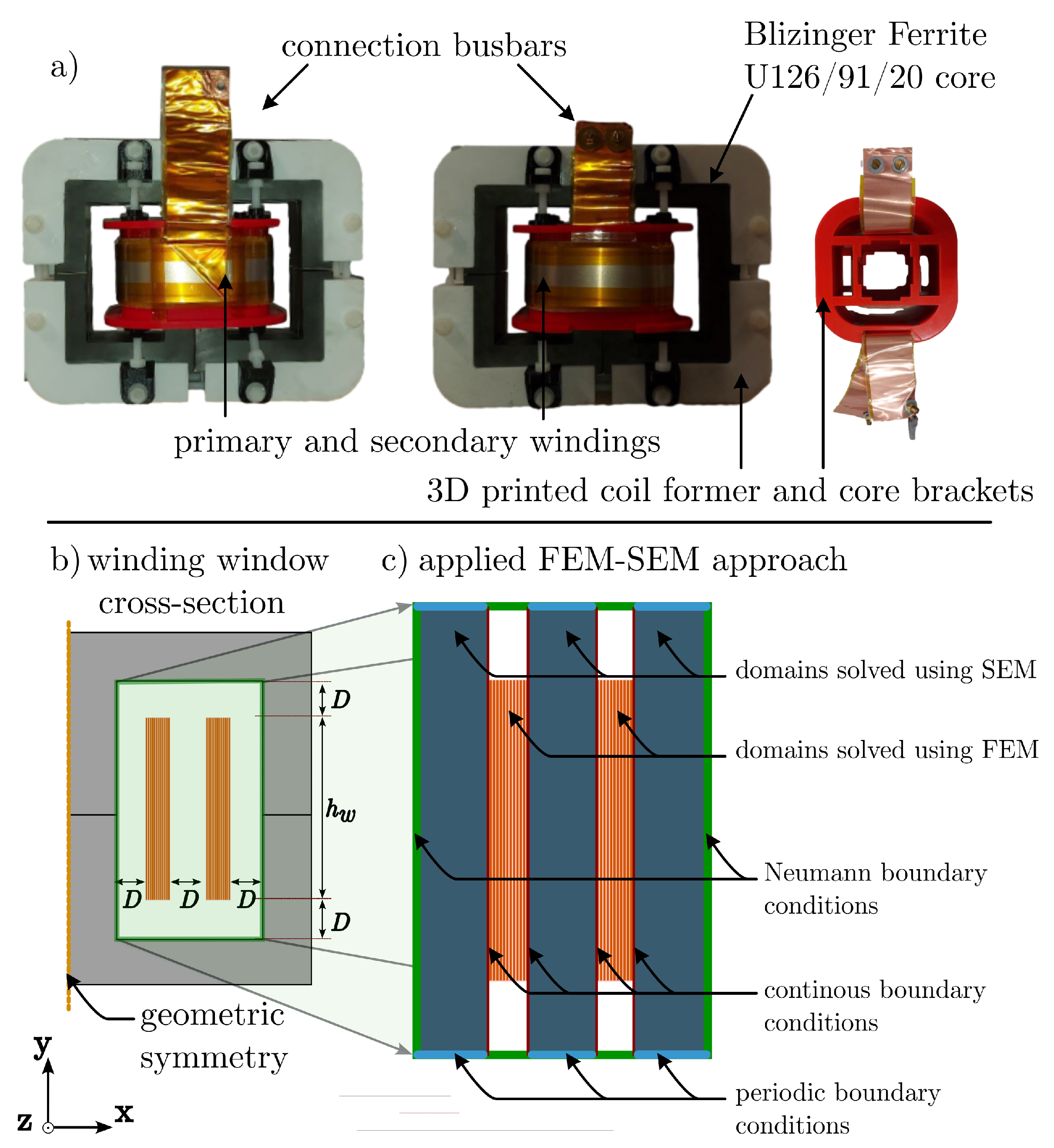
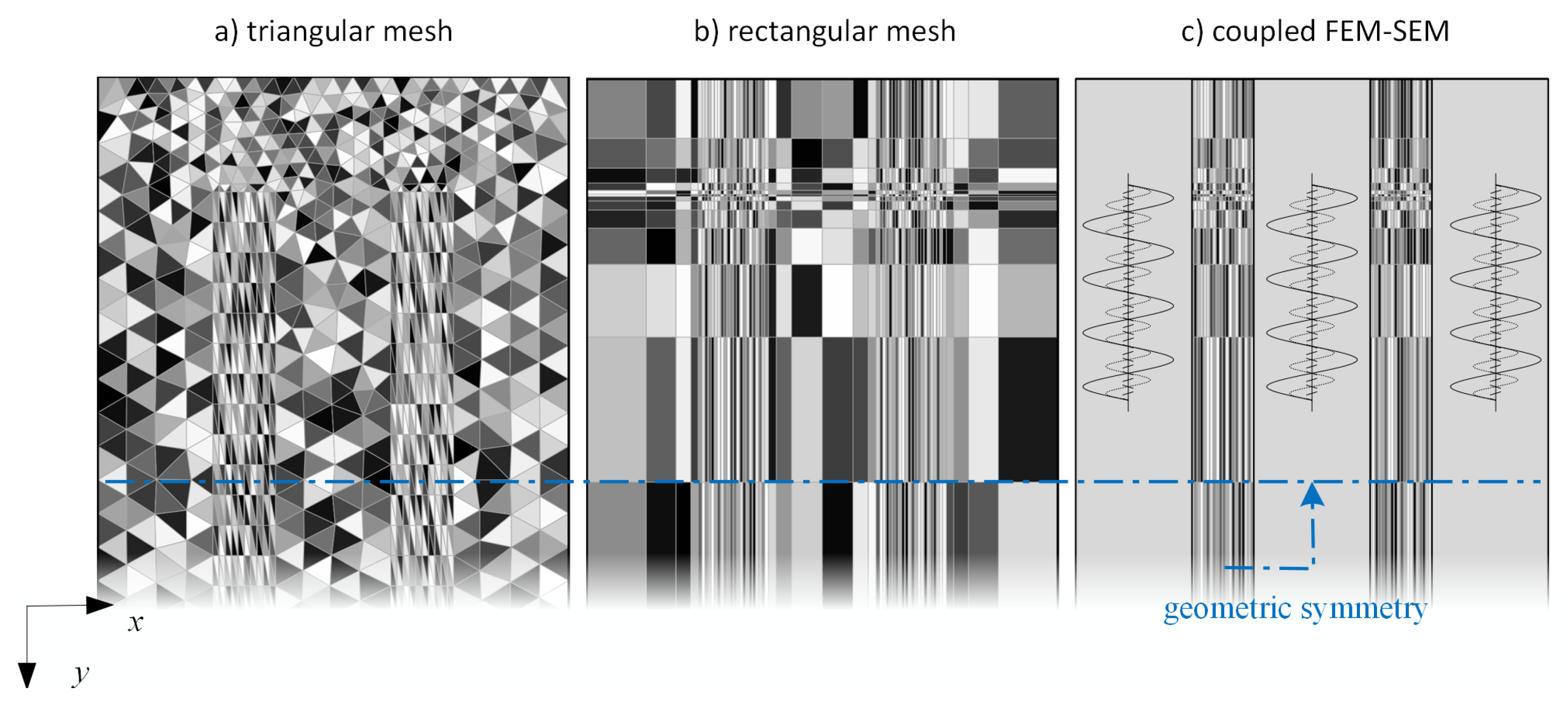
• An FEM model was implemented across all regions of the winding window, which was named ${\Omega }_{\mathrm{FEM}}$. This model compares triangular and rectilinear mesh types with a focus on the computational efficiency and accuracy (see Figure 2a,b).
• A hybrid FEM–SEM model was developed, ${\Omega }_{\mathrm{SEM}}$, including the clearance distances, where the SEM was coupled with the FEM model employed on the winding regions (see Figure 2c).

Figure 1. (a) The MFT under-study, (b) the cross-section area of the MFT winding, (c) the graphical representation of applied FEM-SEM.

Figure 1. (a) The MFT under-study, (b) the cross-section area of the MFT winding, (c) the graphical representation of applied FEM-SEM.

Figure 2. Meshes generated using (a) triangular elements and (b) rectilinear elements; (c) a hybrid FEM–SEM model. All three discretizations exhibit equal number of elements for the geometry depicted in Figure 1.

Figure 2. Meshes generated using (a) triangular elements and (b) rectilinear elements; (c) a hybrid FEM–SEM model. All three discretizations exhibit equal number of elements for the geometry depicted in Figure 1.

By investigating the appropriate meshing approach and incorporating the results using the hybrid FEM–SEM, the computational effort and precision involved in analyzing the magnetic field and the current density distribution within medium-frequency transformers were addressed. The subsequent subsections provide a concise overview of the derived system of equations utilized in this research.

3.1. Solution of MQS Formulation Using FEM

To model the induced eddy current distribution on ${\Omega }_{\mathrm{FEM}}$ using the FEM, we multiply (1) by a test function $\beta$, integrate over ${\Omega }_{\mathrm{FEM}}$, and apply integration by parts to the Laplace term:

$${\int \int }_{{\Omega }_{FEM}}\frac{1}{\mu }\nabla A_{\mathrm{z}}·\nabla \beta d\Omega +{\int }_{\Gamma }\frac{1}{\mu }\frac{\partial A_{\mathrm{z}}}{\partial n}·\beta d\Gamma -{\int \int }_{{\Omega }_{FEM}}j\omega \sigma A_{\mathrm{z}}·\beta d\Omega +{\int \int }_{{\Omega }_{{\mathrm{c}}_n}}\sigma v_n·\beta d\Omega =0,$$

(5)

where ${\Omega }_{\mathrm{FEM}}={\Omega }_{\mathrm{c}}\cup {\Omega }_{\mathrm{nc}}$, which has ${\Omega }_{\mathrm{c}}$ and ${\Omega }_{\mathrm{nc}}$ as conducting and nonconducting regions, respectively.

Additionally, the interconnection of the conductors and the relation between the current and voltage drop at the terminals of the windings are enforced using Lagrange multipliers. The conditions are the following:

• The current flowing through the winding $\mathrm{j}$ is uniform:
  $i_n-i_{\mathrm{s},\mathrm{j}}=0$ for every conductor n belonging to the winding $\mathrm{j}$, where $i_{\mathrm{s},\mathrm{j}}$ is the source current at the terminal of winding $\mathrm{j}$.
• The voltage drops of the conductors, $v_n$, belonging to the winding $\mathrm{j}$ add up to the terminal voltage drop of the winding $\mathrm{j}$, $V_{\mathrm{s},\mathrm{j}}$:

  $$V_{\mathrm{s},\mathrm{j}}-\sum v_n=0.$$

The mesh and the residual of the weak form (5) are interconnected using numerical methods such as the FEM, where the mesh influences the local accuracy of the numerical approximation and affects the magnitude of the residual, thereby representing the error between the approximate and exact solution. While a dense mesh does not necessarily reduce the error, it does significantly increase the computational effort. The right balance between accuracy and complexity can be obtained by choosing the appropriate mesh type and size resulting from a mesh convergence analysis.

Triangular meshing algorithms are the most widespread in commercial FEM modules. However, they can be challenging when applied to structured geometries, which consist of regular shapes like rectangles or cylinders. Aligning triangular elements with straight boundaries and parallel lines and the transition from a dense mesh to a coarse mesh in regions with less accuracy requirements in structured geometries can be inefficient, thereby leading to lower mesh quality and potential numerical instabilities or unnecessary computations. In contrast, generating a structured mesh and mesh refinement is typically straightforward for structured geometries.

3.2. Spectral Element Method Formulation

In MFTs with large clearance distances and fine foil thicknesses, as illustrated in Figure 1, a coupling between the SEM implemented in [13] and the FEM, named the FEM–SEM, can improve the efficiency of the analysis, since the clearance regions do not require high mesh densities. In this approach, the transformer domain is divided into different regions: the bulk regions, where the FEM is employed to handle the foil windings, and the nonconducting regions, where the SEM is applied to account for clearance distances. The FEM accurately captures the complex behavior of current density distribution within the winding regions, while the SEM excels in accurately representing the magnetic field distribution in the nonconducting regions. In the developed 2D SEM model, the solution of the magnetic vector potential, $A_{\mathrm{z}}$, and the flux density, $B_{\mathrm{x}}$, in ${\Omega }_{\mathrm{SEM}}$, are represented using the position-dependent complex Fourier coefficients as follows [17]:

$$A_{\mathrm{z}}=acos\left(\mathit{K}y\right)cos\left(\mathit{K}x\right),$$

(6)

and

$$B_{\mathrm{x}}=\frac{\partial A_{\mathrm{z}}}{\partial y}=-a\mathit{K}cos\left(\mathit{K}y\right)sin\left(\mathit{K}x\right),$$

(7)

where a is the vector of unknown Fourier coefficients, $\mathit{K}$ is the diagonal matrix containing $k_{n}x$ or $k_{n}y$ elements, and $k_n=(n\pi /\tau )$, having $\tau$ as the periodic width of the ${\Omega }_{\mathrm{SEM}}$. Consequently, the set of equations that guarantees the continuity of $A_{\mathrm{z}}$ and $\frac{\partial A}{\partial n}$ on the FEM–SEM coupling boundaries, ${\Gamma }_{\mathrm{c}}$, is derived. On the edge boundaries, ${\Gamma }_{\mathrm{b}}$, the Neumann boundary condition ($\frac{\partial A}{\partial n}=0$) is applied, thus forcing the vanishing of ${\int }_{{\Gamma }_{\mathrm{b}}}\frac{\partial A}{\partial n}d\Gamma$ in (5) [18]. On the coupling boundaries, ${\Gamma }_{\mathrm{c}}$, the boundary integral ${\int }_{{\Gamma }_{\mathrm{b}}}\frac{\partial A}{\partial n}$ in (5) is added to the residual using (7), which forces the boundary integral in (5) to the solution of the SEM, since $\frac{\partial A}{\partial n}{\Gamma }_{\mathrm{b}}=B_{\mathrm{x}}{\Gamma }_{{\mathrm{b}}_{\mathrm{SEM}}}$, thereby contributing to the residual, $\mathcal{R}$, as follows:

$$\mathcal{R}+=\frac{1}{\mu }{\int }_{{\Gamma }_{\mathrm{c}}}(\frac{\partial A^{FEM}}{\partial n}-B_{\mathrm{x}}^{SEM})d\Gamma .$$

(8)

Finally, the coupling of the two sets of equations is achieved by imposing the continuity of the solution of $A_{\mathrm{z}}$ on ${\Gamma }_{\mathrm{c}}$ using a Lagrange multiplier, $\lambda$:

$$\mathcal{R}+={\int }_{{\Gamma }_c}\lambda (A_{\mathrm{z}}^{SEM}-A_{\mathrm{z}}^{FEM})d\Gamma .$$

(9)

4. Results

To implement a computational comparison of the aforementioned modeling methods and the mesh shapes, a set of study cases was developed in accordance to a laboratory-scale MFT prototype. The MFT was composed of a ferrite core and a set of primary and secondary windings. Foil conductors were used in the windings, and the 2D cross-section of the winding window was used to represent the electromagnetic behavior of the MFT. The laboratory-scale MFT prototype and the graphical representation of the study case are shown in Figure 1. The dimensional specifications of the MFT 1, MFT 2, and MFT 3 test benches are provided in

Table 1. Dimensional specifications of the MFT benchmarks.

Dimensions	Symbol	MFT 1	MFT 2	MFT 3
Mumber of winding turns	$N_1/N_2$	10/10	10/10	10/10
Foil thickness	$d_{\mathrm{w}}$	1 [mm]	0.2 [mm]	1 [mm]
Foil height	$h_{\mathrm{w}}$	100 [mm]	100 [mm]	100 [mm]
Interlayer insulation thickness	$d_{\mathrm{ins}}$	0.2 [mm]	0.2 [mm]	0.2 [mm]
Windings–core clearance distance	D	20 [mm]	20 [mm]	50 [mm]
Core window height	$h_{\mathrm{c}}$	140 [mm]	140 [mm]	200 [mm]

. In order to investigate the influence of different geometric specifications on the accuracy and computational performance of the developed models, the foil thickness and the clearance distance in MFT 1 were adjusted in MFT 2 and MFT 3, respectively. This adjustment demonstrates the impact of the skin depth of the foil conductors and the field deviation due to the clearance distances on the global resistance and the inductance of the MFT. The developed FEM and hybrid FEM–SEM systems of equations were used to estimate the winding loss and the magnetic energy of the MFT. Due to the high relative permeability (${\mu }_r$) of the ferrite core and the operation of the MFTs in the linear region of the material characteristics, the winding window can be modeled by assuming an infinite permeability for the core. Thus, the ferromagnetic core geometry can be replaced by Neumann boundary conditions on the boundaries of the winding window.

In the conducted simulations, the computational tasks were executed on a system equipped with an Intel core i5 CPU featuring four cores and coupled with 16 GB of RAM.

To thoroughly assess the trade-off between the computational cost and the accuracy of the FEM models employing triangular and rectilinear meshes, as well as the hybrid FEM–SEM method, an FEM reference model with an extra-fine rectangular mesh was initially generated. This reference model served as a basis for mesh refinements and computational performance evaluations.

To conduct a comprehensive comparison of the performance outcomes of the models developed, a series of simulations with both fine and coarse mesh elements was conducted using both triangular and rectilinear meshing approaches. In order to ensure a fair comparison, the number of degrees of freedom in the winding conductors was maintained at comparatively similar levels for equivalent models employing fine and coarse, triangular, and rectilinear meshes. Moreover, the hybrid FEM–SEM model was tailored to suit the specific characteristics of the MFT under investigation, thereby utilizing two levels of fine and coarse discretization. The models were then solved within the medium-frequency range of 1 kHz to 50 kHz, thereby allowing for the computation of the AC resistance and reactance, which are the crucial parameters in analyzing the overall performance of any electromechanical device in this frequency range. The computed values and corresponding deviations of the AC resistance and reactance are plotted in Figure 3.

The resistance values calculated from the FEM with the rectangular mesh and FEM–SEM models consistently confirmed their accuracy, irrespective of the level of discretization they involved in all three cases. However, it is evident that when the triangular mesh was employed, the resistance calculation tended to lose its accuracy for frequencies exceeding 10 kHz, except for MFT 2. This is due to the fact that, in MFT 2, the thickness of the foil conductors dropped to 0.2 mm, which resulted in a relatively lower skin effect. Thus, the relative error in computing the resistance was dropped in the so-called FEM-Tri fine and coarse, in conformity with the reduction of the induced eddy effects. In addition, upon comparing the performance of the FEM–SEM for the three cases, there was a noticeable increase in the relative error of computing the AC resistance using the hybrid model with increases in the frequency. However, compared to the triangular mesh, the coupled FEM–SEM approach showed a higher relative error with a reduced eddy current in MFT 2. We assert that this behavior is the result of the Gibbs phenomena [19] rooted in the Fourier series, which will be addressed in the next section. Among all the MFT models, both the fine and coarse triangular meshes exhibited a maximum error slightly below 30% in terms of the calculated resistance, thereby indicating a higher degree of approximation error compared to the other meshes in the frequency of 50 kHz. This demonstrates that the triangular FEM simulations require a larger number of degrees of freedom to achieve comparable levels of accuracy to compute the current density distribution on the foil windings in higher-frequency ranges. In contrast, the coarse rectilinear mesh demonstrated a significantly smaller deviation, thereby showcasing its ability to provide more accurate results using a similar number of degrees of freedom (dof) in a wide range of frequencies.

Conversely, when it came to calculating the magnetic energy, all the models and configurations of the dof consistently yielded results within a range of comparable accuracy. This is due to the fact that the inductance of the system is less dependent on the frequency. Yet, the results with the triangular mesh showed the highest inconsistency with respect to the increase in frequency. Even though the FEM–SEM approach with a coarse discretization showed the largest discrepancy of up to 8% for the frequency of 50 kHz, the consistency of the errors makes it a preferable choice when compared to the FEM with a triangular mesh.

To gain a deeper understanding of the computational performance of these three methods, considering both the accuracy and the size of the system of equations, a comprehensive investigation was conducted. The findings are visually depicted in Figure 4 and are detailed in the upcoming section.

5. Discussion

In Figure 4a, the 2D distribution of the magnetic vector potential in the winding window area was plotted for the FEM with a rectangular mesh. The FEM-Recti model utilizes a fine rectilinear mesh to capture the intricate details of the magnetic field. However, upon comparing the results in Figure 4b,c, although both the FEM-Tri and FEM–SEM models posed a similar number of dof, they showed deviations from FEM-Recti model results in Figure 4a. For the FEM–SEM method solution, the discrepancy was specifically along the edges of the conductors on the coupling boundaries, thereby indicating the presence of the Gibbs phenomenon. Furthermore, what distinguishes the Gibbs phenomenon is that this overshoot did not diminish with increasing refinements, i.e., as more sinusoidal terms were added to the series [19]. The occurrence of the Gibbs phenomenon manifested as an error near the edges of the conductors, thereby resulting in a deviation from the expected results in Figure 3.

In the case of FEM with triangular meshes, even though both the FEM-Recti and FEM-Tri use the same system of equations to solve the problem, the importance of choosing the right mesh shape becomes evident. In the FEM-Recti model, the transition from a fine mesh to a coarse mesh in nonconducting regions is simple. Thus, a rectilinear meshing approach efficiently refines the mesh in the area with foil windings, where the precise computation of $A_{\mathrm{z}}$ is crucial, and reduces the mesh density in no-conducting regions accordingly. On the other hand, the FEM-Tri model requires a relatively larger number of meshes in nonconducting regions due to the intricacies of accommodating a triangular mesh as compared to a rectangular one, thereby resulting in the lower accuracy in the conducting regions.

The hybrid FEM–SEM model exceled in terms of the number of unknowns employed and the computational efficiency it provided when compared to the traditional FEM models, as can be seen in

Table 2. Number of degrees of freedom (dof) for different meshes.

Mesh Type	Extra-Fine	Fine	Coarse
Triangular	-	21,872	8310
Rectilinear	28,444	15,795	7422
FEM–SEM	-	6950	5478

. However, the FEM with rectangular mesh shapes also delivered competitive results due to its accuracy, irrespective of the number of degrees of freedom used. In contrast, the FEM with a triangular mesh lagged in terms of both the accuracy and degrees of freedom when subjected to comparison.

To enhance the comparative analysis of the proposed methods, we assessed the convergence by examining the error in the computed resistance and reactance for the studied case, MFT 1, which is depicted in Figure 5. As the level of discretization (dof) increased, a noticeable reduction in the computed error relative to the reference resulted, which was obtained with the extra-fine rectilinear mesh elements and observed across all the investigated methods. The FEM-Recti and FEM–SEM simulations exhibited the most rapid reduction in relative error for both the resistance and reactance. Conversely, the FEM with triangular elements demonstrated a slower convergence rate with increasing dof. Additionally, the simulation time required to solve the systems of equations was analyzed for various dof, as presented in Figure 5. The FEM-Recti outperformed the FEM-Tri and FEM–SEM in terms of solution time for similar relative errors, thereby underscoring the significance of the chosen solver type. Certainly, the choice of solver significantly influences solution times, as it is impacted by factors such as matrix sparsity and the distribution of unknowns within the different approaches. Therefore, comparing the dof provides a more equitable basis for evaluating and contrasting these methods, as it directly demonstrates the dimensions of the system of equations.

Concluding our comparative study,

Table 3. A qualitative comparison of available approaches and the proposed method.

Method	Accuracy	Flexibility	Computational Cost	Simplicity
Dowell’s Method [6]	-	*	***	***
Empirical Methods [7,8,9,10,11]	*	**	**	**
SEM [13]	**	***	**	**
FEM-Tri	***	***	**	**
FEM-Recti	***	***	***	***
Proposed FEM–SEM Approach	***	***	***	***

offers a qualitative analysis of the previous methods in the literature alongside the developed methods in this study in terms of the accuracy, the flexibility of the method regarding various geometrical specifications, computational costs, and the simplicity of implementation of the methods. The FEM with rectilinear mesh elements and the FEM–SEM solution emerged as the most preferable in terms of accuracy and flexibility.

6. Conclusions

This study addressed the significance of meshing approaches in the analysis of structured geometries, such as foil windings, by developing two MQS models for the medium-frequency range. The models utilize an FEM approach with triangular and rectilinear meshes and a hybrid FEM–SEM to improve the computational efficiency and accuracy. The results validated the accuracy and reliability of the implemented FEM–SEM and FEM with rectangular mesh models, while also highlighting discrepancies in the FEM with triangular mesh method despite a similar number of unknowns used to solve the problem. The developed models were successfully applied to estimate the winding loss and magnetic energy in MFTs with foil windings. The results revealed that the hybrid FEM–SEM approach surpassed the accuracy of conventional FEM models using triangular meshes. Additionally, it offers computational efficiency advantages, from the aspect of dof, over FEM models. Furthermore, it holds the potential for solving problems in scenarios such as 3D geometries, where direct solvers are not always feasible due to limited amounts of RAM.

This study contributes to the advancement of computational modeling techniques for analyzing eddy currents in MFTs and provides valuable insights into the meshing challenges associated with such analyses. The developed models and findings offer a foundation for future research and optimization of the computational approaches applied to MFTs.

References

1. Huber, J.E.; Kolar, J.W. Applicability of Solid-State Transformers in Today’s and Future Distribution Grids. IEEE Trans. Smart Grid 2019, 10, 317–326. [Google Scholar] [CrossRef]
2. Rothmund, D.; Guillod, T.; Bortis, D.; Kolar, J.W. 99% Efficient 10 kV SiC-Based 7 kV/400 V DC Transformer for Future Data Centers. IEEE J. Emerg. Sel. Top. Power Electron. 2019, 7, 753–767. [Google Scholar] [CrossRef]
3. Mogorovic, M.; Dujic, D. 100 kW, 10 kHz Medium-Frequency Transformer Design Optimization and Experimental Verification. IEEE Trans. Power Electron. 2019, 34, 1696–1708. [Google Scholar] [CrossRef]
4. Pourkeivannour, S.; Drofenik, U.; Curti, M.; Lomonova, E.A. Design Trade-Off Analysis of Dry-Type Medium Frequency Transformers with Parallel Foil Windings. In Proceedings of the International Conference on Electrical Machines (ICEM), Valencia, Spain, 5–8 September 2022; pp. 2149–2154. [Google Scholar]
5. Pourkeivannour, S.; Curti, M.; Drofenik, U.; Cremasco, A.; Lomonova, E.A. Mitigation of Circulating Currents in Parallel Foil Windings for Medium Frequency Transformers. IEEE Trans. Magn. 2022, 58, 1–4. [Google Scholar] [CrossRef]
6. Dowell, P.L. Effects of eddy currents in transformer windings. Proc. Inst. Electr. Eng. 1966, 113, 1387. [Google Scholar] [CrossRef]
7. Schlesinger, R.; Biela, J. Comparison of Analytical Models of Transformer Leakage Inductance: Accuracy Versus Computational Effort. IEEE Trans. Power Electron. 2021, 36, 146–156. [Google Scholar] [CrossRef]
8. Guo, X.; Li, C.; Zheng, Z.; Li, Y. General Analytical Model and Optimization for Leakage Inductances of Medium-Frequency Transformers. IEEE J. Emerg. Sel. Top. Power Electron. 2022, 10, 3511–3524. [Google Scholar] [CrossRef]
9. Bennett, E.; Larson, S.C. Effective resistance to alternating currents of multilayer windings. Electr. Eng. 1940, 59, 1010–1016. [Google Scholar] [CrossRef]
10. Ferreira, J.A.; van Wyk, J.D. A new method for the more accurate determination of conductor losses in power electronic converter magnetic components. In Proceedings of the Third International Conference on Power Electronics and Variable-Speed Drives, London, UK, 13–15 July 1988; pp. 184–187. [Google Scholar]
11. Bahmani, M.A.; Thiringer, T.; Ortega, H. An Accurate pseudoempirical model of winding loss calculation in HF foil and round conductors in switch mode magnetics. IEEE Trans. Power Electron. 2017, 11, 540–547. [Google Scholar]
12. Wang, T.; Yuan, W.; Yuan, J. A Novel Semi-Analytical Method for Foil Winding Losses Calculation Considering Edge Effect in Medium Frequency Transformers. IEEE Trans. Magn. 2022, 58, 1–9. [Google Scholar] [CrossRef]
13. Pourkeivannour, S.; Curti, M.; Custers, C.; Cremasco, A.; Drofenik, U.; Lomonova, E.A. A Fourier-based Semi-Analytical Model for Foil-Wound Solid-State-Transformers. IEEE Trans. Magn. 2021, 9464, 1–5. [Google Scholar] [CrossRef]
14. Silvester, P.P.; Ferrari, R.L. Finite Elements for Electrical Engineers, 3rd ed.; Cambridge University Press: Cambridge, UK, 1996. [Google Scholar]
15. Bermúdez, A.; Gómez, D.; Salgado, P. Mathematical Models and Numerical Simulation in Electromagnetism; Springer: New York, NY, USA, 2014. [Google Scholar]
16. van Zwieten, J.S.B.; van Zwieten, G.J.; Hoitinga, W. Nutils (8.0). Zenodo. 2023. Available online: https://zenodo.org/records/10068507 (accessed on 10 December 2023).
17. Custers, C.H.H.M.; Jansen, J.W.; Lomonova, E.A. 2-D Semi-Analytical Modeling of Eddy Currents in Multiple Non-Connected Conducting Elements. IEEE Trans. Magn. 2017, 53, 1–6. [Google Scholar] [CrossRef]
18. Touzani, R.; Rappaz, J.; Applications, W.S. Mathematical Models for Eddy Currents and Magnetostatics; Springer: Dordrecht, The Netherlands, 2014. [Google Scholar]
19. Jerri, A.J. Lanczos-like σ-factors for reducing the Gibbs phenomenon in general orthogonal expansions and other representations. JoCAAA 2000, 2, 111–127. [Google Scholar]
Figure 3. The AC resistance R and reactance X of (a) MFT 1 (b) MFT 2, and (c) MFT 3 computed using extra-fine, fine, and coarse mesh elements with triangular and rectilinear shapes, as well as the hybrid FEM–SEM method and the corresponding deviations from the extra-fine reference model.
J 06 00041 g003
Figure 4. The distribution of A z at the frequency of 50 kHz, which was solved using (a) FEM employing a rectangular mesh ( A z FEM Recti ), (b) the pointwise deviation of coupled FEM–SEM method ( A z FEM SEM ), and (c) with FEM utilizing a triangular mesh ( A z FEM Tri ); both compared with A z FEM Recti .
J 06 00041 g004
Figure 5. The comparison of computational costs for FEM with triangular and rectangular meshes, as well as the hybrid FEM–SEM model, solved for the test bench MFT 1 at the frequency of 20 kHz.
J 06 00041 g005