Relationship between Sunspot Numbers and Mean Annual Precipitation: Application of Cross-Wavelet Transform—A Case Study


Department of Civil and Environmental Engineering and Construction, University of Nevada, Las Vegas, NV 89154, USA
*
Author to whom correspondence should be addressed.
J 2020, 3(1), 67-78; https://doi.org/10.3390/j3010007
Submission received: 8 January 2020
/
Revised: 6 February 2020
/
Accepted: 13 February 2020
/
Published: 15 February 2020
Abstract
:Observations show that the Sun, which is the primary source of energy for the Earth’s climate system, is a variable star. In order to understand the influence of solar variability on the Earth’s climate, knowledge of solar variability and solar–terrestrial interactions is required. Knowledge of the Sun’s cyclic behavior can be used for future prediction purposes on Earth. In this study, the possible connection between sunspot numbers (SSN) as a proxy for the 11-year solar cycle and mean annual precipitation (MAP) in Iran were investigated, with the motivation of contributing to the controversial issue of the relationship between SSN and MAP. Nine locations throughout Iran were selected, representing different climatic conditions in the country. Cross-wavelet transform (XWT) analysis was employed to investigate the temporal relationship between cyclicities in SSN and MAP. Results indicated that a distinct 8–12-year correlation exists between the two time series of SSN and MAP, and peaks in precipitation mostly occur one to three years after the SSN maxima. The findings of this study can be beneficial for policymakers, to consider future potential droughts and wet years based on sunspot activities, so that water resources can be more properly managed.
1. Introduction
The Sun, as a dynamic object, shows different degrees of activity in its convection zone, surface (photosphere), and atmosphere [1]. Solar variability can be classified as short-term (e.g., solar flares), intermediate, and long-term, covering a wide temporal range, from minutes to even millions and billions of years. Examples of the long-term solar variations include the 11-year Schwabe cycle (sunspot cycle), 22-year Hale cycle, 80 to 90-year Gleissberg cycle, ~180 to 200-year de Vries cycle, etc. [2]. Sunspots appear as dark spots on the surface of the Sun. They have temperatures as low as ~4200 K, compared to ~6050 K for the surrounding quiet photosphere, and they typically last between several days to several weeks. The magnetic strengths in the sunspots can be thousands of times stronger than the Earth’s magnetic field. Figure 1 shows images taken by the Solar and Heliospheric Observatory (SOHO) spacecraft, and compares sunspots on the Sun’s surface (top row) and ultraviolet light radiating from the solar atmosphere (bottom row) at the solar maximum in the year 2000 (left column), and at the solar minimum in the year 2009 (right column) [3].
There have been many arguments about how the 11-year sunspot cycle, and the 22-year Hale cycle affect Earth’s climate and local weather conditions [1,4,5]. Diverse climatic parameters on Earth show near 11, 22, 80, and 210-year periodicities, which are also frequent in solar activity time series [6].
During the 11-year solar cycle, the amount of solar energy absorbed in the UV part of the spectrum within the upper stratosphere varies from 6 to 8%. This variation in solar energy output is believed to be one of the most important factors influencing the Earth’s climate. Solar ultraviolet (UV) variability results in direct variations in irradiance and indirect variations in stratospheric ozone, as well as changes the vertical and horizontal temperature structures [7,8,9]. These changes in the thermal gradients, and consequently in the wind systems, lead to changes in the vertical propagation of the planetary waves that drive the global circulation [10,11].
One key element that can be used to prove this possible connection is the impact of solar activity on meteorological parameters. This can be determined by analyzing records of solar activity indicators such as sunspot numbers (SSN), and terrestrial meteorological records such as mean annual precipitation (MAP).
1.1. Previous Studies
The National Academy of Sciences panel on solar variability, weather, and climate studied the possible connection between solar variability and climatic conditions on Earth, and concluded that solar variability can alter the weather and climate on our planet [12]. In the analyses of observational data, the existence of 11-year solar cycle signals in the meteorological fields of the lower atmosphere has been confirmed [13,14,15,16,17,18].
Among pioneer studies in this field, in 1989, Barnett reported that tropospheric biennial oscillation (TBO) is modulated by an 11-year solar cycle [19]. Moreover, in 1997, Svensmark and Friis-Christensen found a correlation between cosmic ray flux fluctuations, which are impacted by sunspot activities as well as increases of both ion-charged rain and aerosols in the Earth’s atmosphere. The authors concluded that the increased cosmic rays’ flux leads to increased cloud cover, and potentially higher precipitation [20]. Furthermore, Gleisner and Thejll used a regression analysis with F10.7 as a measure of solar activity, and found that there is a significant response of the troposphere to the 11-year solar cycle [15]. They found that in the tropics and at mid-latitudes, solar forcing is the strongest. Moreover, their study revealed that during higher solar (HS) years, the tropical meridional overturning of the atmosphere is somewhat weaker and broader in a latitudinal extent. Similar to the 3 to 5-year period governing the El Niño–Southern Oscillation (ENSO), the quasi-decadal oscillation (QDO) of the 9 to 13-year period in the Earth’s climate system has been found in the tropical Pacific Ocean. These variabilities and the associated tropical warming, have been found fluctuating in phase with the approximately 11-year period signal in the Sun’s total irradiance [21,22,23,24]. In a continuation of Barnett’s work, Kodera suggested that this modulation of the TBO is derived from a difference in the extension of ENSO-related variation into the Indian Ocean [25].
In 2005, Dima et al. used different sea surface temperature (SST) datasets and applied different statistical techniques, to identify two distinct modes of climate variability: one mode was defined by them as ‘the solar mode,’ which was associated with the sunspot cycle; and the other was defined as ‘the internal mode,’ which was linked to atmosphere-ocean interaction. According to them, sea level pressure and upper atmospheric levels were dominated by the ‘solar mode,’ whereas ‘the internal mode’ explained the oceanic surface temperature with approximately three times more variance than that of the solar mode [26]. Furthermore, Kodera et al. found that during HS activity years, the ENSO-related signal is confined in the Pacific sector. They also showed that during the period of lower solar (LS) activity, ENSO-related variability extends into the Indian Ocean [27].
In another study, Alexander et al. found a statistically significant 21-year periodicity in South African annual rainfall, river flow, and lake levels, and the Southern Oscillation Index [28]. Moreover, Perry found linkage in the midwestern United States between the time series of galactic cosmic rays, and the regional climate [29]. Furthermore, Prokoph et al. studied the maximum annual streamflow records in southern Canada and found that major floods most often occurred between six and seven years after the last solar maximum, during low SSN periods [30]. More recently, Li et al. studied how El Niño events and solar activity affected extreme precipitation in typical regions of the Loess Plateau in China. The authors found that at peak sunspot number events, there was the highest amount of precipitation [31]. In 2018, Dong et al. used wavelet techniques to analyze the annual and decadal variations of the hydrological processes in the Yoshino River basin in Japan, to determine any interactions with either solar activity or ENSO. The authors found that both solar activity and El Niño could influence hydrological patterns, since strong cross power and high coherence were observed between hydrological variability and SSN/SST in the periodicities of 2–7 and 11 years [32]. In another study in 2019, Li et al. studied the correlation between tree rings and solar activity, using the Hilbert transform and variational mode decomposition (VMD) methods. The authors concluded that tree ring growth is a function of sunspot activity, and the width of tree rings is influenced by other external environments [33].
1.2. Objectives
Based on the literature review, there is an increasing need to understand the relationship between SSN and the changes in hydrologic variables that follow, specifically in the interest of efficiently managing sustainable water resources. Analyzing the hydrologic and helio-physical time series is a complex task, considering that they do not always follow what are considered normally distributed probability functions, as well as not being stationary in nature. Recently, much attention has been given to improving the prediction of trend patterns and periodicities in this type of time series data, using wavelet analysis techniques. In this regard, by employing the wavelet analysis, and implementing the cross-wavelet transform (XWT) method, this study aims to investigate the possible connection between SSN and MAP over a wide geographic scale and in different climate regions, in the case study of Iran.
2. Materials and Methods
2.1. Case Study and Data
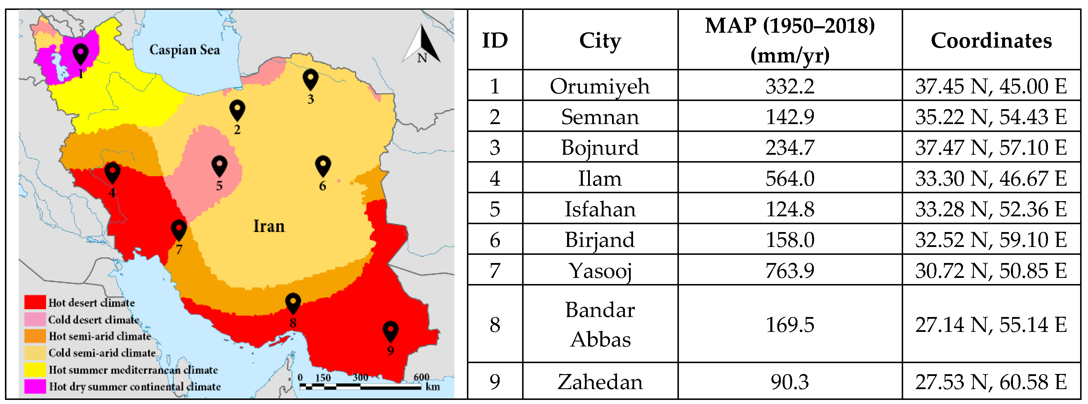
Iran is located in the mid-latitudes of the Earth’s arid and semi-arid regions. Meteorological records show that the average MAP in Iran was approximately 250 mm/yr from 1950 to 2018, which is about one-third of the global average [34]. In this study, in order to cover the whole extent of the country for analyzing the potential connection between SSN and MAP, nine locations that have the longest data records available were selected. These areas are located in high, middle, and low latitudes, and have different climatic conditions (Figure 2). The MAP and SSN time series for each station are presented in Figure 3. For this study, the precipitation data were provided by the Islamic Republic of Iran Meteorological Organization (IRIMO) and covered the time period from 1950 to 2018 [35]. Yearly mean SSN records were retrieved from the World Data Center for the production, preservation, and dissemination of the international sunspot number [36].
2.2. Wavelet Analysis
Wavelet analysis can be a powerful tool to analyze processes that are nonstationary in nature, and that occur over finite spatiotemporal domains. In particular, it is used to study oscillatory behavior and reveal periodicities present in signals. The possible correlations between periodic behaviors that are manifest in environmental datasets provide a need for the application of wavelet analysis. A wavelet is a wave-like oscillatory function, which is localized in time and frequency space, and must have a zero mean. The output is a graphical representation of the 95% confidence level contour, which shows the correlation between two time series, as a function of the signal period and its time evolution [37].
Wavelets are flexible functions that are resolved in the time and frequency domains, and thus, ideal for quantifying changes in the contribution of each period (or frequency) over time to the overall variance (or power) of a signal (e.g., a time series). Because wavelets can be scaled (i.e., contracted or dilated), they can efficiently accommodate both high and low-frequency structures in nonstationary signals, whose statistical characteristics vary over time. In this study, the Morlet wavelet was used, which is defined as:
where i is the imaginary unit, t represents nondimensional time, and = 6 is the nondimensional frequency [37]. The continuous wavelet transform of a discrete time series x(t), with equal spacing δt and length T is defined as the convolution of x(t) with a normalized Morlet wavelet [37,38]:
where * indicates the complex conjugate. By varying the wavelet scale s (i.e., dilating and contracting the wavelet), and translating along localized time position τ, one can calculate the wavelet coefficients Wx(s,τ), which describe the contribution of the scales s to the time series x(t) at different time positions τ [37,39]. Here, is a parameter used to normalize the Morlet wavelet function to unit variance, in order to allow direct comparisons of the wavelet coefficients Wx(s,τ) across the different scales s and time positions τ [37,38]. These wavelet coefficients can be used to compute the bias-corrected local wavelet power, which describes how the contribution of each frequency or period in the time series varies in time [37,39,40]:
where 2s is the bias correction factor [40]. The local wavelet power spectrum can then be visualized via contour plots [38,39]. The scale s of the Morlet wavelet is related to Fourier frequency f [39,41]:
When = 6, the scale s is approximately equal to the reciprocal of the Fourier frequency f [39,41]: s ≈ . Hence, in all equations, the scale s can be converted to Fourier frequency f ≈ or period P = ≈ s.
2.2.1. Zero-Padding and the Cone of Influence
In practice, the continuous wavelet transform is computed by using discrete Fourier transforms to calculate all T convolutions simultaneously [37]. However, since the Fourier transform assumes that the data is periodic, errors in the estimation of the local wavelet power spectrum will occur at the beginning and end of any finite-length time series [37,39]. In order to limit these edge effects, the end of a time series is padded with zeros prior to taking the wavelet transform, and the zeroes are then removed [37,39]. Typically, enough zeros are added in order for the total length T of the time series to reach the next-higher power of two. This limits edge effects and improves the speed of the Fourier transform method [37]. Although padding with zeros limits errors due to edge effects, it introduces artificial discontinuities at the endpoints of the data [37,39]. As one gets closer to the end of the data, more zeros are included in the estimation of the local wavelet spectrum, thus reducing its reliability [37,39]. The region where zero padding affects the estimation of the wavelet spectrum is called the cone of influence (COI), and is defined as the region in which the wavelet power for a discontinuity at the edge drops by a factor of e−2 [37]. Hence, any region falling below the COI is susceptible to edge effects.
2.2.2. Statistical Significance Testing
In order to determine the statistical significance of the wavelet spectrum obtained from a time series, one must first formulate an appropriate null hypothesis. Here, the null hypothesis is that the observed time series is generated by a stationary process, with a given background power spectrum P(k) [37,38]. Since many ecological and environmental time series exhibit strong temporal autocorrelation [42,43], in this study, a first-order autoregressive model was used to generate a temporally auto-correlated time series, or red noise, which served as the null hypothesis. Specifically, the power spectrum P(k) of the red noise process was calculated with [44]:
where the autocorrelation coefficient α at time lag 1 is estimated from the observed time series and k = 0, …, N/2 represents the frequency index. The observed wavelet spectrum can be compared to the wavelet spectrum of the red noise process by means of a chi-square test. The distribution of the local wavelet power spectrum of a red noise process is [37]:
where k represents the frequency index, σ2 represents the variance of the time series, “→” means “is distributed as,” and represents the chi-square distribution with two degrees of freedom. The value of P(k) is the mean wavelet power spectrum at frequency k that corresponds to the wavelet scale s [37]. Using this equation, one can construct 95% confidence contour lines at each scale using the 95th percentile of the chi-square distribution [37].
2.2.3. Wavelet Coherence
Wavelet coherence can be used to quantify the strength of the covariation between two signals in the time and frequency domains [37,38,45]. To compute the wavelet coherence, one must first calculate the cross-wavelet of time series x(t) and y(t), by taking their respective wavelet transforms Wx(s,τ) and Wy(s,τ). Then, the cross-wavelet transform is computed via [37,38]:
where * indicates complex conjugation. The wavelet coherence between two time series x(t) and y(t), with wavelet spectra Wx(s,τ) and Wy(s,τ), and cross-wavelet spectrum Wx,y(s,τ), is then computed as [38,39,45]:
where denotes smoothing in both time τ and scale s and 0 ≤ (s,τ) ≤ 1. The time smoothing uses a filter given by the absolute value of the wavelet function at each scale, normalized to have a total weight of unity, which is a Gaussian function for the Morlet wavelet. The scale smoothing is done with a boxcar function of width 0.6, which corresponds to the decorrelation scale of the Morlet wavelet [37,38,45]. Overall, the wavelet coherence can be thought of as the local, or time-resolved correlation between two time series [39,46,47].
3. Results and Discussion
The wavelet transform (WT) has been a major development in the field of data analysis since the 1980s. WT is an effective means to process time-series data, especially those with nonstationary characteristics [48]. Iran has been experiencing high climate variations during the past decades. However, the changes differed from region to region over the country. Precipitation records in Figure 3 showed that from 1950 to 2018, MAP in all stations in Iran was highly nonstationary and nonlinear, which had no clear periodic fluctuation. Unlike MAP, SSN showed a clear period. To deconstruct the original data and analyze the period of SSN and MAP, the XWT method was employed. XWT analyses on the SSN and MAP were performed in MATLAB. The power spectrum of this analysis is displayed in Figure 4. In the figure, a black, thick contour designates a 5% significance level. Additionally, the COI is shown by lighter shades, and the arrows represent the relative phase relationship between the two time series. Right (left) pointing arrows show an in-phase (anti-phase) relationship. Warmer colors (e.g., yellow) show stronger correlations, while colder colors (e.g., blue) show weaker correlations. Visual inspection indicates that in all stations, an 8–12-year reoccurrence pattern is apparent, therefore suggesting a connection between sunspot activities and the terrestrial climate in the study area. Correlations in stations number 3, 5, and 6 are less significant, which could be attributed to their geographic locations. These stations are located in either a hot desert climate, or cold semi-arid climate regions. Moreover, some of the stations exhibit cyclicities other than 8–12 years. However, the strongest correlation still exists in the 8–12 year band.
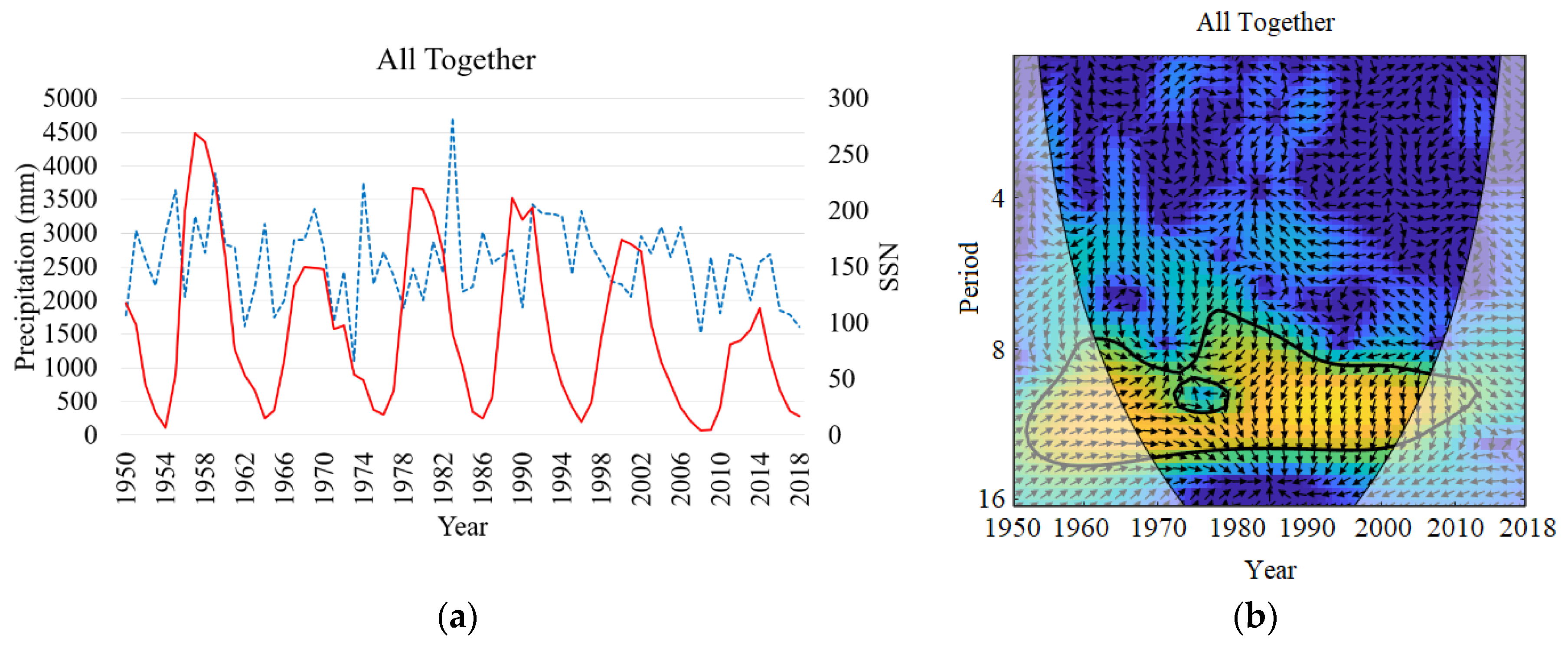
Furthermore, in order to investigate the connection between SSN and MAP in the whole extent of the country, the MAP time series of all nine stations were combined (Figure 5a) and analyzed with the SSN to find common cyclicities. Figure 5b presents the XWT analysis result, and shows an apparent 8–12-year reoccurrence pattern. These changes in radiation and energy balance affect components of the water cycle, and the climate.
The time series in Figure 3 and Figure 5a show that peaks in precipitation mostly occurred one to three years after the SSN maxima. These are in accordance with the findings of Li and Yang [49], who also reported that the annual precipitation at the Yellow River showed hysteresis for sunspot numbers. Moreover, Zhang et al. [50] reported that, at the peak of sunspot activity or two years near it, the summer precipitation in Xi’an, China, increased sharply. Li et al. also reported that at the peak of sunspot number or two years near it, the precipitation in the Yan’an area in Chana increased [31].
Climate variations can affect different sectors such as agriculture and energy, directly or indirectly. Therefore, they have to be assessed and managed properly. Jamali et al. showed that lack of adaptation to climate variations leads to a considerable decrease in efficiency in Iran’s Karkheh Hydropower in the future [51]. Some examples of a lack of insufficient climate assessment studies and improper managements in Iran are: damages caused by heavy rains; floods and damages on many houses, infrastructure, water and power supply; groundwater depletion; droughts and their impacts on food quality and quantity, economy, health, and people’s livelihood; drying lakes; sand storms; and ecosystem degradation [52,53,54,55,56,57,58,59,60,61,62]. These issues indicate the necessity of implementing sustainable adaptation and mitigation plans, considering possible variations in climate.
Various attempts have been made to decipher and explain the reasons behind the relationship between sunspot numbers and hydrological parameters on Earth, and research in this area is still ongoing [63,64]. White et al. found that the tropical global-average temperature of the upper ocean (0.1 °C) is not driven by the approximately 11-year period signal in surface solar radiative forcing, but rather indirectly by a greater warming of the tropical troposphere temperature (0.2–0.5 °C) in response to the approximately 11-year period signal in the Sun’s UV radiative forcing of the lower stratosphere temperature (1.0 °C) via absorption by ozone [65]. Furthermore, observations of global cloud cover and cosmic rays’ flux show that over 11-year sunspot cycles, there is a negative correlation with the solar irradiance flux [66,67]. This correlation can also be one of the possible reasons for the change in hydrological parameters on Earth during certain solar cycles. Finally, considering a global large-scale pattern, change in Walker circulation, Hadley circulation, jet movement, local proximity to the ocean, local temperature, etc., all could contribute to rainfall in any location of the Earth. Hence in the future, it could be interesting to see which could be a dominating factor to contribute decadal rainfall patterns in Iran.
4. Conclusions
In order to investigate the connection between the 11-year sunspot activity cycle and precipitation patterns from 1950 to 2018 in Iran, the XWT technique was employed. For this analysis, SSN records were used as indicators of the solar activity level. The results indicated that an approximately 11-year cyclicity exists between the two series, and there is a possible link between precipitation patterns and the number of sunspots. The time series also showed that peaks in precipitation mostly occurred one to three years after the SSN maxima. Even though the stations studied in this research are located in different climate regions, the same conclusion applies to all of them. However, there are more factors that affect MAP than SSN, such as anthropogenic factors (e.g., combustion of fossil fuels, human-driven changes in land use and land cover, urban heat island effects, etc.), ENSO, and variability within geosphere dynamic equilibriums. Therefore, sunspot activities should not be translated directly into climate and precipitation changes, but are a likely influence, through a series of non-linear oceanic-atmospheric responses.
For future studies, since the climatology of precipitation varies in seasons, it is recommended that the impact of SSN on precipitation patterns be studied seasonally as well. A similar approach, as the methodology of the present paper, can be implemented in other regions of the world with different climatic conditions, where the relationship between SSN and MAP has not yet been studied.
Author Contributions
Conceptualization, M.N.-S.; methodology, M.N.-S.; software, M.N.-S.; writing—Original draft preparation, M.N.-S.; writing—Review and editing, M.K.; supervision, M.K.; All authors have read and agreed to the published version of the manuscript.
Funding
The publication fees for this article were supported by the UNLV University Libraries Open Article Fund.
Conflicts of Interest
The authors declare no conflict of interest.
References
- Gray, L.J.; Beer, J.; Geller, M.; Haigh, J.D.; Lockwood, M.; Matthes, K.; Cubasch, U.; Fleitmann, D.; Harrison, G.; Hood, L.; et al. Solar influences on climate. Rev. Geophys. 2010, 48, RG4001. [Google Scholar] [CrossRef]
- Tsiropoula, G. Signatures of solar activity variability in meteorological parameters. J. Atmos. Sol. Terr. Phys. 2003, 65, 469–482. [Google Scholar] [CrossRef]
- Sunspots at Solar Maximum and Minimum. Available online: https://earthobservatory.nasa.gov/images/37575/sunspots-at-solar-maximum-and-minimum/ (accessed on 25 January 2020).
- Lean, J.; Rind, D. Evaluating sun–climate relationships since the Little Ice Age. J. Atmos. Sol. Terr. Phys. 1999, 61, 25–36. [Google Scholar] [CrossRef]
- Rind, D.; Lean, J.; Lerner, J.; Lonergan, P.; Leboissitier, A. Exploring the stratospheric/tropospheric response to solar forcing. J. Geophys. Res. 2008, 113. [Google Scholar] [CrossRef] [Green Version]
- Casa, A.D.; Nasello, O. Low frequency oscillation of rainfall in Córdoba, Argentina, and its relation with solar cycles and cosmic rays. Atmos. Res. 2012, 113, 140–146. [Google Scholar] [CrossRef]
- Haigh, J.D. The impact of solar variability on climate. Science 1996, 272, 981–984. [Google Scholar] [CrossRef]
- Balachandran, N.K.; Rind, D.; Lonergan, P.; Shindell, D.T. Effects of solar cycle variability on the lower stratosphere and the troposphere. J. Geophys. Res. 1999, 104, 321–339. [Google Scholar] [CrossRef]
- Shindell, D.; Rind, D.; Balachandran, N.; Lean, J.; Lonergan, P. Solar cycle variability, ozone and climate. Science 1999, 284, 305–308. [Google Scholar] [CrossRef] [Green Version]
- Kodera, K.; Kuroda, Y. Dynamical response to the solar cycle: Winter stratopause and lower stratosphere. J. Geophys. Res. 2002, 107, 4749. [Google Scholar] [CrossRef] [Green Version]
- Matthes, K.; Langematz, U.; Gray, L.J.; Kodera, K.; Labitzke, K. Improved 11-year solar signal in the Freie Universität Berlin Climate Middle Atmosphere Model (FUB-CMAM). J. Geophys. Res. 2004, 109, D06101. [Google Scholar] [CrossRef]
- National Research Council. Solar Variability, Weather and Climate; National Academic Press: Washington, DC, USA, 1982. [Google Scholar]
- Van Loon, H.; Shea, D.J. The global 11-yr solar signal in July–August. Geophys. Res. Lett. 2000, 27, 2965–2968. [Google Scholar] [CrossRef]
- Haigh, J.D. The effects of solar variability on the Earth’s climate. Philos. Trans. R. Soc. Lond. Ser. A. 2003, 361, 95–111. [Google Scholar] [CrossRef]
- Gleisner, H.; Thejll, P. Patterns of tropospheric response to solar variability. Geophys. Res. Lett. 2003, 30, 1711. [Google Scholar] [CrossRef]
- Crooks, S.A.; Gray, L.J. Characterisation of the 11-year solar signal using a multiple regression analysis of the ERA-40 dataset. J. Clim. 2005, 18, 996–1015. [Google Scholar] [CrossRef]
- Seleshi, Y.; Demaree, G.R. Sunspot numbers as a possible indicator of annual rainfall at Addis Ababa, Ethiopia. Int. J. Climatol. 1993, 14, 911–923. [Google Scholar] [CrossRef]
- Gachari, F.; Mulati, D.; Mutuku, J.N. Sunspot numbers: Implications on Eastern African rainfall. S. Afr. J. Sci. 2014, 110. [Google Scholar] [CrossRef] [Green Version]
- Barnett, T.P. A solar-ocean relation: Fact or fiction. Geophys. Res. Lett. 1989, 16, 803–806. [Google Scholar] [CrossRef]
- Svensmark, H.; Friis-Christensen, E. Variation of cosmic ray flux and global cloud coverage—A missing link in solar-climate relationships. J. Atmos. Sol. Terr. Phys. 1997, 59, 1225–1232. [Google Scholar] [CrossRef]
- White, W.B.; Lean, J.; Cayan, D.R.; Dettinger, M.D. Response of global upper ocean temperature to changing solar irradiance. J. Geophys. Res. Oceans 1997, 102, 3255–3266. [Google Scholar] [CrossRef]
- White, W.B.; Cayan, D.R.; Lean, J. Global upper ocean heat storage response to radiative forcing from changing solar irradiance and increasing greenhouse gas/aerosol concentrations. J. Geophys. Res. 1998, 103, 355–366. [Google Scholar] [CrossRef]
- Allan, R.J. ENSO and climate variability in the last 150 years. In El Nino and the Southern Oscillation: Multiscale Variability, Global and Regional Impacts; Cambridge University Press: New York, NY, USA, 2000; pp. 3–55. [Google Scholar]
- White, W.B.; Tourre, Y.M. Global SST/SLP waves during the 20th century. Geophys. Res. Lett. 2003, 30, 1651. [Google Scholar] [CrossRef]
- Kodera, K. Solar influence on the Indian Ocean monsoon through dynamical processes. Geophys. Res. Lett. 2004, 31, L24209. [Google Scholar] [CrossRef] [Green Version]
- Dima, M.; Lohmann, G.; Dima, I. Solar-induced and internal climate variability at decadal time scales. Int. J. Climatol. 2005, 25, 713–733. [Google Scholar] [CrossRef]
- Kodera, K.; Coughlin, K.; Arakawa, O. Possible modulation of the connection between the Pacific and Indian Ocean variability by the solar cycle. Geophys. Res. Lett. 2007, 34, L03710. [Google Scholar] [CrossRef]
- Alexander, W.J.R.; Bailey, F.; Bredenkamp, D.B.; van der Merwe, A.; Willemse, N. Linkages between solar activity, climate predictability and water resource development. J. S. Afr. Inst. Civ. Eng. 2007, 49, 32–44. [Google Scholar]
- Perry, C.A. Evidence for a physical linkage between galactic cosmic rays and regional climate time series. Adv. Space Res. 2007, 40, 353–364. [Google Scholar] [CrossRef]
- Prokoph, A.; Adamowski, J.; Adamowski, K. Influence of the 11 year solar cycle on annual streamflow maxima in Southern Canada. J. Hydrol. 2012, 442–443, 55–62. [Google Scholar] [CrossRef]
- Li, H.J.; Gao, J.E.; Zhang, H.C.; Zhang, Y.X.; Zhang, Y.Y. Response of Extreme Precipitation to Solar Activity and El Nino Events in Typical Regions of the Loess Plateau. Adv. Meteorol. 2017, 2017, 9823865. [Google Scholar] [CrossRef]
- Dong, L.; Fu, C.; Liu, J.; Zhang, P. Combined Effects of Solar Activity and El Niño on Hydrologic Patterns in the Yoshino River Basin, Japan. Water Resour. Manag. 2018, 32, 2421–2435. [Google Scholar] [CrossRef]
- Li, G.; Zheng, M.; Yang, H. Cycle Analysis Method of Tree Ring and Solar Activity Based on Variational Mode Decomposition and Hilbert Transform. Adv. Meteorol. 2019, 2019, 1715673. [Google Scholar] [CrossRef]
- Moghim, S. Impact of climate variation on hydrometeorology in Iran. Glob. Planet. Chang. 2018, 170, 93–105. [Google Scholar] [CrossRef]
- I.R. of IRAN Meteorological Organization. Available online: http://www.irimo.ir/eng/ (accessed on 18 February 2018).
- World Data Center for the Production. Preservation and Dissemination of the International Sunspot Number. Available online: http://www.sidc.be/silso/ (accessed on 18 February 2018).
- Torrence, C.; Compo, G.P. A Practical Guide to Wavelet Analysis. Bull. Am. Meteorol. Soc. 1998, 79, 61–78. [Google Scholar] [CrossRef] [Green Version]
- Grinsted, A.; Moore, J.C.; Jevrejeva, S. Application of the cross wavelet transform and wavelet coherence to geophysical time series. Nonlinear Process. Geophys. 2004, 11, 561–566. [Google Scholar] [CrossRef]
- Cazelles, B.; Chavez, M.; Berteaux, D.; Menard, F.; Vik, J.O.; Jenouvrier, S.; Stenseth, N.C. Wavelet analysis of ecological time series. Oecologia 2008, 156, 287–304. [Google Scholar] [CrossRef]
- Liu, Y.; San Liang, X.; Weisberg, R.H. Rectification of the Bias in the Wavelet Power Spectrum. J. Atmos. Ocean. Technol. 2007, 24, 2093–2102. [Google Scholar] [CrossRef]
- Maraun, D.; Kurths, J. Cross wavelet analysis: Significance testing and pitfalls. Nonlinear Process. Geophys. 2004, 11, 505–514. [Google Scholar] [CrossRef] [Green Version]
- Beninca, E.; Johnk, K.D.; Heerkloss, R.; Huisman, J. Coupled predator-prey oscillations in a chaotic food web. Ecol. Lett. 2009, 12, 1367–1378. [Google Scholar] [CrossRef]
- Ruokolainen, L.; Lindén, A.; Kaitala, V.; Fowler, M.S. Ecological and evolutionary dynamics under coloured environmental variation. Trends Ecol. Evolut. 2009, 24, 555–563. [Google Scholar] [CrossRef]
- Gilman, D.L.; Fuglister, F.J.; Mitchell, J.M. On the Power Spectrum of “Red Noise”. J. Atmos. Sci. 1963, 20, 182–184. [Google Scholar] [CrossRef] [Green Version]
- Torrence, C.; Webster, P.J. The annual cycle of persistence in the El Niño/Southern Oscillation. Q. J. R. Meteorol. Soc. 1998, 124, 1985–2004. [Google Scholar] [CrossRef]
- Rouyer, T.; Fromentin, J.M.; Menard, F.; Cazelles, B.; Briand, K.; Pianet, R.; Planque, B.; Stenseth, N.C. Complex interplays among population dynamics, environmental forcing, and exploitation in fisheries. Proc. Natl. Acad. Sci. USA 2008, 105, 5420–5425. [Google Scholar] [CrossRef] [PubMed] [Green Version]
- Rouyer, T.; Fromentin, J.M.; Stenseth, N.C.; Cazelles, B. Analysing multiple time series and extending significance testing in wavelet analysis. Mar. Ecol. Prog. Ser. 2008, 359, 11–23. [Google Scholar] [CrossRef]
- Percival, D.B.; Walden, A.T. Wavelet Methods for Time Series Analysis; Cambridge University Press: Cambridge, UK, 2006. [Google Scholar]
- Li, C.H.; Yang, Z.F. Relationship between sun activities and natural runoff Yellow river basin based on Morlet wavelet. J. Water Resour. Water Eng. 2004, 15, 1–4. [Google Scholar]
- Zhang, X.N.; Shi, X.M.; Yang, S.Y. Relationship between number of sunspots and rainfall in Xi’an in summer and autumn. Arid Zone Res. 2013, 30, 485–490. [Google Scholar]
- Jamali, S.; Abrishamchi, A.; Madani, K. Climate Change and Hydropower Planning in the Middle East: Implications for Iran’s Karkheh Hydropower Systems. J. Energy Eng. 2013, 139, 153–160. [Google Scholar] [CrossRef]
- Nazari-Sharabian, M.; Taheriyoun, M.; Ahmad, S.; Karakouzian, M.; Ahmadi, A. Water Quality Modeling of Mahabad Dam Watershed–Reservoir System under Climate Change Conditions, using SWAT and System Dynamics. Water 2019, 11, 394. [Google Scholar] [CrossRef] [Green Version]
- Nazari-Sharabian, M.; Taheriyoun, M.; Karakouzian, M. Surface Runoff and Pollutant Load Response to Urbanization, Climate Variability, and Low Impact Developments—A Case Study. Water Supply 2019, 19, 2410–2421. [Google Scholar] [CrossRef]
- Nazari-Sharabian, M.; Ahmad, S.; Karakouzian, M. Climate Change and Eutrophication: A Short Review. Eng. Tech. Appl. Sci. Res. 2018, 8, 3668–3672. [Google Scholar] [CrossRef]
- Motagh, M.; Djamour, Y.; Walter, T.R.; Wetzel, H.U.; Zschau, J.; Arabi, S. Land subsidence in Mashhad Valley, northeast Iran: Results from InSAR, levelling and GPS. Geophys. J. Int. 2007, 168, 518–526. [Google Scholar] [CrossRef]
- Tourian, M.J.; Elmi, O.; Chen, Q.; Devaraju, B.; Roohi, S.H.; Sneeuw, N. A spaceborne multisensor approach to monitor the desiccation of Lake Urmia in Iran. Remote Sens. Environ. 2015, 156, 349–360. [Google Scholar] [CrossRef]
- Delju, A.H.; Ceylan, A.; Piguet, E.; Rebetez, M. Observed climate variability and change in Urmia Lake Basin, Iran. Theor. Appl. Climatol. 2013, 111, 285–296. [Google Scholar] [CrossRef] [Green Version]
- Zarghami, M. Effective watershed management; Case study of Urmia Lake, Iran. Lake Reserv. Manag. 2011, 27, 87–94. [Google Scholar] [CrossRef]
- Naimabadi, A.; Ghadiri, A.; Idanie, E.; Babaei, A.A.; Alavi, N.; Shirmardi, M.; Khodadadi, A.; Marzouni, M.B.; Ankali, K.A.; Rouhizadeh, A.; et al. Chemical composition of PM10 and its in vitro toxicological impacts on lung cells during the Middle Eastern Dust (MED) storms in Ahvaz, Iran. Environ. Pollut. 2016, 211, 316–324. [Google Scholar] [CrossRef] [PubMed]
- Najafi, M.S.; Khoshakhllagh, F.; Zamanzadeh, S.M.; Shirazi, M.H.; Samadi, M.; Hajikhani, S. Characteristics of TSP Loads during the Middle East Springtime Dust Storm (MESDS) in Western Iran. Arab. J. Geosci. 2014, 7, 5367–5381. [Google Scholar] [CrossRef]
- Shinn, E.A. Coral reef recovery in Florida and the Persian Gulf. Environ. Geol. 1976, 1, 241–254. [Google Scholar] [CrossRef]
- Mostafavi, P.G.; Fatemi, S.M.R.; Shahhosseiny, M.H.; Hoegh-Guldberg, O.; Loh, W.K.W. Predominance of clade D Symbiodinium in shallow-water reef-building corals off Kish and Larak Islands (Persian Gulf, Iran). Mar. Biol. 2007, 153, 25–34. [Google Scholar] [CrossRef]
- Roy, I. The role of the sun in atmosphere-ocean coupling. Int. J. Climatol. 2014, 34, 655–677. [Google Scholar] [CrossRef] [Green Version]
- Roy, I. Solar cyclic variability can modulate winter Arctic climate. Sci. Rep. Nat. Publ. 2018, 8, 4864. [Google Scholar] [CrossRef]
- White, W.B.; Dettinger, M.D.; Cayan, D.R. Sources of global warming in the upper-ocean on decadal period scales. J. Geophys. Res. 2003, 108, 3248. [Google Scholar] [CrossRef] [Green Version]
- Marsh, N.D.; Svensmark, H. Low Cloud Properties Influenced by Cosmic Rays. Phys. Rev. Lett. 2000, 85, 5004–5007. [Google Scholar] [CrossRef] [Green Version]
- Carslaw, K.S. Cosmic Rays, Clouds, and Climate. Science 2002, 298, 1732–1737. [Google Scholar] [CrossRef] [Green Version]
Figure 1.
(a,c): the Sun during solar maximum (19 July 2000), with high sunspot numbers (SSN); (b,d): the Sun during solar minimum (18 March 2009), with low SSN [3].
Figure 1.
(a,c): the Sun during solar maximum (19 July 2000), with high sunspot numbers (SSN); (b,d): the Sun during solar minimum (18 March 2009), with low SSN [3].

Figure 2.
Selected stations in the study area [35].
Figure 2.
Selected stations in the study area [35].

Figure 4.
Cross-wavelet transform (XWT) analysis results in selected stations.
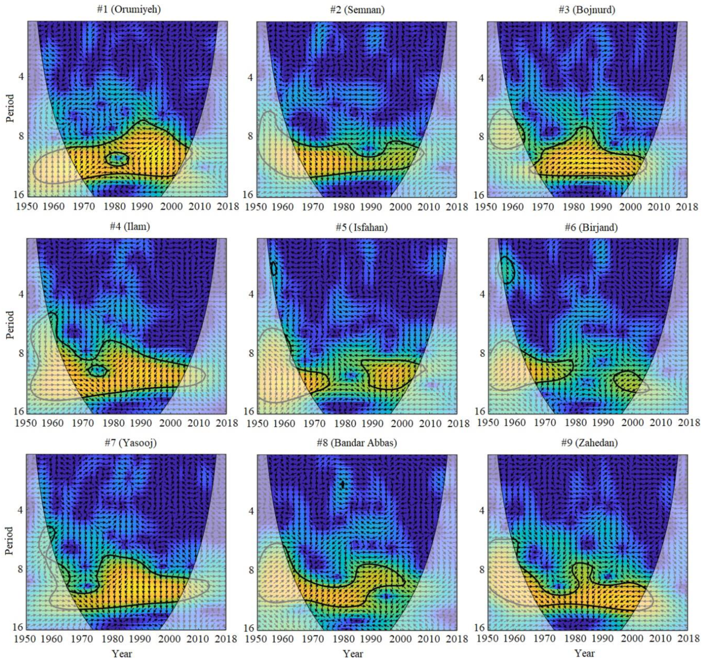
Figure 5.
(a) SSN and MAP of all stations combined, and (b) the XWT analysis result of the two time series.
Figure 5.
(a) SSN and MAP of all stations combined, and (b) the XWT analysis result of the two time series.
© 2020 by the authors. Licensee MDPI, Basel, Switzerland. This article is an open access article distributed under the terms and conditions of the Creative Commons Attribution (CC BY) license (http://creativecommons.org/licenses/by/4.0/).
Share and Cite
MDPI and ACS Style
Nazari-Sharabian, M.; Karakouzian, M. Relationship between Sunspot Numbers and Mean Annual Precipitation: Application of Cross-Wavelet Transform—A Case Study. J 2020, 3, 67-78. https://doi.org/10.3390/j3010007
AMA Style
Nazari-Sharabian M, Karakouzian M. Relationship between Sunspot Numbers and Mean Annual Precipitation: Application of Cross-Wavelet Transform—A Case Study. J. 2020; 3(1):67-78. https://doi.org/10.3390/j3010007
Chicago/Turabian StyleNazari-Sharabian, Mohammad, and Moses Karakouzian. 2020. "Relationship between Sunspot Numbers and Mean Annual Precipitation: Application of Cross-Wavelet Transform—A Case Study" J 3, no. 1: 67-78. https://doi.org/10.3390/j3010007