Monitoring and Modeling of Saline-Sodic Vertisol Reclamation by Echinochloa stagnina

Abstract

Soil salinity due to irrigation is a major constraint to agriculture, particularly in arid and semi-arid zones, due to water scarcity and high evaporation rates. Reducing salinity is a fundamental objective for protecting the soil and supporting agricultural production. The present study aimed to empirically measure and simulate with a model, the reduction in soil salinity in a Vertisol by the cultivation and irrigation of Echinochloa stagnina. Laboratory soil column experiments were conducted to test three treatments: (i) ponded bare soil without crops, (ii) ponded soil cultivated with E. stagnina in two successive cropping seasons and (iii) ponded soil permanently cultivated with E. stagnina with a staggered harvest. After 11 months of E. stagnina growth, the electrical conductivity of soil saturated paste (ECe) decreased by 79–88% in the topsoil layer (0–8 cm) in both soils cultivated with E. stagnina and in bare soil. In contrast, in the deepest soil layer (18–25 cm), the ECe decreased more in soil cultivated with E. stagnina (41–83%) than in bare soil (32–58%). Salt stocks, which were initially similar in the columns, decreased more in soil cultivated with E. stagnina (65–87%) than in bare soil (34–45%). The simulation model Hydrus-1D was used to predict the general trends in soil salinity and compare them to measurements. Both the measurements and model predictions highlighted the contrast between the two cropping seasons: soil salinity decreased slowly during the first cropping season and rapidly during the second cropping season following the intercropping season. Our results also suggested that planting E. stagnina was a promising option for controlling the salinity of saline-sodic Vertisols.

1. Introduction

Irrigated land degradation by salinization is a major constraint for agricultural production on irrigated soils, particularly in arid and semi-arid zones. Most of the reduction in crop yield is caused by salt accumulation in soil [1]. It has been estimated that 33% of irrigated agricultural land worldwide is afflicted by high salinity for various reasons, including low precipitation, high surface evaporation, weathering of native rocks, irrigation with saline water, and unsuitable cultural practices [2]. Clayey soils, such as vertic soils in the Niger River valley, which are irrigated for rice production in Niger, are particularly exposed to salinization because of their low hydraulic conductivity at water saturation which inhibits salt leaching [3,4]. The salinization process of vertic soils has been observed in irrigated perimeters of the Niger River valley and leads to the abandonment of agricultural land [5,6].

Economic and environmental challenges of irrigated land salinity have led to the development of several approaches to promote soil conservation and limit soil salinity. Many engineering-based remediation techniques have been developed to reclaim salt-affected soils, including physical, chemical, and biological remediation [7]. The last technique includes approaches such as phytodesalinization, which uses salt-tolerant plants or halophytes to decrease soil salinity and thus increase crop production [8,9,10,11]. This approach is increasingly investigated, both in field studies [12,13,14,15] and under controlled laboratory conditions [10,16,17,18] since water ponding is difficult to apply in water-limited areas and less effective in fine-textured soils [4,19,20].

The processes underlying phytodesalinization have been reported by several authors [11,21] and include (i) the improvement of soil structure by root expansion, which promotes salt leaching; (ii) salt export in plant biomass, (iii) an increase in CO₂ partial pressure within the root zone and (iv) root proton release (for N2-fixing plants). However, the relative importance of these processes, particularly salt leaching and salt accumulation in plant biomass, has not yet been addressed well. Moreover, for Vertisols, phytodesalinization is influenced by shrink–swell processes, which govern water flow and solute transfer. Furthermore, the high clay content of Vertisols may limit plant root development [22].

Many studies have used simulation models to investigate water flow and salt dynamics in clay soils [23,24,25,26,27]. Few, however, have simulated salt dynamics in salt-affected soils undergoing remediation techniques. The Hydrus-1D model has been used to predict the effects of gypsum amendments on increasing the hydraulic conductivity and decreasing the salinity of clay saline-sodic soils [28,29]. Hydrus-1D has also been coupled with the UNSATCHEM module to simulate the Ca, Na, Mg and K contents of sodic Vertisols reclaimed with gypsum amendments and irrigated with water of varying quality. However, most existing studies have not considered the potential effects of plants to predict the salt dynamics in soil–plant systems, the plant-root modification of soil structure to improve salt leaching, or their high capacity to accumulate salts in their biomass.

Echinochloa stagnina is a perennial semi-aquatic grass characterized by a C4 photosynthetic metabolism. It develops a dense fasciculated root system which can colonize the soil profile even at depth. This dense root system can improve soil structure, i.e., increase soil porosity to favor preferential water flows towards a greater depth [15]. It is a fodder crop characterized by a high productivity (20 to 40 t/ha of dry matter) and a high nutritional value [30,31]. The E. stagnina plant is able to grow in salt-affected land. Indeed, several authors have reported the high phytoreclamation potential of E. stagnina in saline-sodic clay soil in Egypt [12] or in sodic soil and saline soil in the Niger River valley [15,32].

The aim of this study was to evaluate and simulate by a modeling approach, the phytodesalinization process of irrigated saline-sodic Vertisols cultivated with E. stagnina. Based on soil column laboratory experiments and simulation modeling, we compared two treatments of ponded cultivated soil columns with a control treatment consisting of bare soil columns.

2. Materials and Methods

2.1. Soil Characteristics

Soil cores used for laboratory experiments were provided from irrigated paddy fields of Kollo (13°16′35.32″ N, 2°21′31.81″ E), located in the Niger River valley 50 km southeast of Niamey (Niger). The soil characteristics (

Table 1. Initial physico-chemical characteristics of soil in the columns.

Clay	Silt	Sand	pH	ECe	Ca2+	Mg2+	Na+	K+	CEC	Org.C	OM	ESP b	SAR a	ESI c
%				dS/m	Cmol/kg					g/kg		%
69.4	25.9	4.7	4.7	15.7	2.7	26.1	3.3	0.3	18.6	7.4	12.8	18.0	0.9	0.9

ECe: electrical conductivity of soil saturated paste, SAR: Sodium Adsorption Ratio, ESP: Exchangeable Sodium Percentage, ESI: Electrochemical Stability Index, ^a SAR = C_Na/[(C_Ca + C_Mg)/2]^1/2, ^b ESP = 100 (E_Na)/CEC, ^c ESI = EC/ESP according to [34]; CEC: cobaltihexamine cation exchange capacity; C: concentration of corresponding exchangeable cation.

) showed that the soil is an acid saline-sodic Vertisol [33] with a high clay content (69.4%), an acid pH (4.7), a high electrical conductivity of soil saturated paste (ECe = 15.7 dS/m), and a low saturated soil hydraulic conductivity (<2.8 × 10⁻⁸ m/s) [4,15]. The high exchangeable sodium percentage (ESP = 18%) shows that the soil is sodic and could have a degraded structure, with soil settling and a low hydraulic conductivity at water saturation induced by clay dispersion.

2.2. Soil Column Sampling

Six undisturbed soil cores were sampled from the topsoil layer (0–25 cm) of an uncultivated plot in the irrigated paddy fields of Kollo, chosen because of their high salinity. The soil columns (16 cm in diameter and 25 cm in height) were collected at the soil field capacity by a conventional coring method using manual pressure and PVC pipes. Each soil column was installed in the laboratory and filled with two layers (Figure 1) according to [35]: (i) a reconstituted topsoil layer (from 0–19 cm) compacted to 1.4 g/cm³ of the bulk density; (ii) an undisturbed soil layer (from 19–25 cm) in which the initial soil structure was conserved.

2.3. Experimental Design

The experimental design was composed of 3 treatments (2 replicates each): (i) ponded bare soil without a crop was considered as a control (CT); (ii) ponded soil cultivated with E. stagnina (CEs) in two successive cropping seasons separated by a total harvest, and (iii) ponded soil permanently cultivated with E. stagnina (CEp) with a staggered harvest every 4 months.

At 5, 15 and 21 cm of soil depth, each column was vertically equipped with a porous ceramic suction cup to extract the soil solution, and with a micro-tensiometer to measure the soil pressure head (Figure 1). The soil solution was collected every 2 weeks with the porous ceramic suction cups, and the pressure head was measured at each depth every 10 min and recorded with an Almemo 5690-2 data logger. The temporal variation in the mass of each soil column and its drainage water (collected at the bottom of the column) was monitored with two digital balances. These masses were also measured every 10 min and recorded with the same Almemo 5690-2 data logger (Figure 1). Each column was set on a gravel layer to facilitate free drainage.

2.4. Crop Production

The experiment was performed for two cropping seasons according to the cutting period of E. stagnina biomass: 4.5 months for each season separated by a 2-month intercropping season.

At the beginning of the first cropping season, saturated soil columns of CEs and CEp were cultivated with E. stagnina plants by transplanting three cuttings (15–20 cm tall) per column. These were grown under controlled conditions: artificial light at 1300 lux (i.e., 1.08 kW/m²) provided for 12 continuous hours per day by two horticultural lamps with 8 neon tubes of 54 W each, located 70 cm above the plants. Room temperature was maintained at 30 °C during the day and 20 °C at night by a radiator on a timer and a thermostat.

During the cropping season, soil irrigation twice per week was performed uniformly on all columns with non-saline water (EC of 0.3–0.4 dS/m), by adjustment of the water layer above the soil surface to 7 cm for each date. These conditions were similar to natural conditions of E. stagnina growth in the Niger River valley.

An inorganic NPK fertilizer (12—15—20) was applied twice per cropping season according to [35], with doses of 200 kg/ha applied one week after planting and of 150 kg/ha one month after the first application. At the end of each cropping season, the yields of aboveground crop biomass (fresh and dry biomass) were evaluated by a harvest of all the biomass on CEs columns and most of the biomass on Cep columns, leaving 10 cm of plant stem at the soil surface which allowed the crop to regenerate during the next season after water irrigation. After the intercropping season, the second cropping season was started by planting new E. stagnina cuttings on CEs columns.

2.5. Soil Sampling and Soil Salinity Monitoring

For the initial state, a composite soil sample was collected from the reconstituted soil of all columns and from the undisturbed soil layer of each column. At the end of the experiment, the columns were destroyed, and soil samples were collected from depths of 0–8, 8–18, and 18–25 cm.

The soil electrical conductivity was measured in a 1:5 soil/water extract (EC_1:5) for each soil sample according to ISO standard 11265 [36]. The soil electrical conductivity measured in the saturated paste (ECe, dS/m) was estimated as:

$${\mathrm{EC}}_{\mathrm{e}}={\mathrm{EC}}_{1:5}\times 5.8$$

(1)

with 5.8 as the conversion factor for clay soils [37].

The EC of the soil solution (ECw), collected with the porous ceramic suction cups, was measured every 2 weeks at 25 °C. The SS was calculated for the 0–8, 8–18 and 18–25 cm soil layers using Equations (2) and (3). First, the total amount of salt in a soil sample (TS, g) was calculated using Equation (2) according to [4] with the relationship:

$$TS=0.0437\times E{C}_{1:5}-0.014$$

(2)

$$SS=\frac{\left(TS\right)}{M}\times BD\times d$$

(3)

with M as the soil sample mass (g), BD as the soil bulk density (g/cm³), and d as the thickness of the soil layer (cm).

2.6. Salt Accumulation in Plant Biomass and Salt Balance in the Soil

The dynamics of plant biomass on the columns (biom) were estimated according to the method in [35] which was used for a logistic model [38] to establish a relationship between the weekly measured plant height, initial biomass, and final biomass. This logistic model was applied to each column and independently for each cropping season using the SSlogis function of R software [39,40].

At the end of each cropping season, the salt amount in the aboveground plant biomass was measured by summing Ca, Na, Mg, K, Cl, P and S biomass concentrations, as reported by [41]. The concentrations of cations (Ca²⁺, Na⁺, Mg^2+, K⁺), anions (Cl⁻, SO₄²⁻, PO₄²⁻ et NO³⁻) and total sulfur (S) were measured in the aboveground plant biomass according to ISO/CEI standard 17025 using (i) inductively coupled plasma atomic emission spectroscopy for Ca, Mg, S, and K and (ii) atomic absorption spectrometry for the other elements.

The salt balance in the soil was estimated weekly from the amount of salt removed in drained water, the amount of salt accumulated in plant biomass, and the salt input from irrigation water. The salt content of drained water and irrigation water was measured weekly using the oven-evaporation method.

2.7. Desalinization during the Intercropping Season by Water Ponding

Water was periodically ponded during the intercropping season to remove salt concentrated on cracked soil. Doses of irrigation water were applied uniformly to all columns. The water was first applied slowly (1.25 mm/h for 4 h) to promote salt leaching from the prism faces by preferential flow and then in a larger dose (2.5–5 mm) until soil saturation, to promote salt dissolution in the soil solution and its leaching. This procedure was performed every 5–10 days for 30 days, with no irrigation between the two ponding cycles. Drained water was collected at the bottom of each column at the end of each ponding cycle to measure its EC and the amount of salt.

2.8. Modeling Approach of Vertisol Desalinization

Hydrus-1D was used to simulate the dynamics of the soil salinity of Vertisols under conditions of permanent water saturation during E. stagnina cropping seasons and under conditions of non-saturation and cracked soil during the intercropping season. A bare soil irrigated at the same frequency as that of cultivated soil was also simulated.

2.8.1. General Model Description

Hydrus-1D [42] is widely used to simulate the dynamics of EC and SS in soil. It numerically solves the Richards equation (Equation (4)) for water flow and uses an advection–dispersion equation (Equation (5)) for solute transport in variably saturated porous media [39].

$$\frac{\partial \theta }{\partial t}=\frac{\partial }{\partial z}\left[K\left(\frac{\partial h}{\partial z}+1\right)\right]-S$$

(4)

with θ as the soil volumetric water content (L3/L3), t as time (T), z as the vertical space coordinate (L), K as the hydraulic conductivity (L/T), h as the pressure head (L), and S as the sink term accounting for root water uptake (L³/L³/T).

$$\frac{\partial \theta C}{\partial t}=\frac{\partial }{\partial t}\left[\theta D\left(\theta ,v\right)\frac{\partial C}{\partial z}-v\theta C\right]-\mathsf{\Gamma } \left(C\right)$$

(5)

with C as the solute concentration of the liquid phase (M/L), D as the dispersion coefficient (L2/T), and $\upsilon$ as the mean pore water velocity (L/T). The dispersion coefficient is defined as:

$$D=\lambda \upsilon$$

(6)

where λ is dispersivity (L), which is considered a material constant independent of the flow rate. Since $\upsilon$ is obtained from predictions of the water flow model (water flux q divided by θ), λ is the only solute transport parameter needed to solve the convection–dispersion equation. It was fixed to a mean value of 0.15 cm following the recommendations of [43] for clay soils.

2.8.2. Soil Hydraulic Properties

Unsaturated soil hydraulic properties were described using van Genuchten–Mualem functional relationships [44,45]:

$$\theta \left(h\right)={\theta }_r+\frac{{\theta }_s-{\theta }_r}{{\left[1+{\left(\alpha h\right)}^n\right]}^m} h<0$$

(7)

$$\theta \left(h\right)={\theta }_{s } h\ge 0$$

(8)

$$K\left(h\right)=K_s{S}_{e }^l{\left[1-{\left(1-S_e^{1/m}\right)}^m\right]}^2$$

(9)

$$S_e=\frac{\theta -{\theta }_r}{{\theta }_s-{\theta }_r}$$

(10)

with ${\theta }_r$ and ${\theta }_s$ as residual and saturated θ (L³/L³), respectively; α (L⁻¹) and n as empirical shape parameters; $m=1-1/n$; l as the pore connectivity parameter assumed to be 0.5 [41] and $S_e$ as the effective saturation.

The parameters ${\theta }_r$, ${\theta }_s$, $\alpha$, n and $K_s$ were estimated for each soil layer in each column for each season using pedotransfer functions predicted by the Rosetta model [46] based on the layer’s particle size distribution (25.9% silt, 69.4% clay, 4.7% sand) and bulk density (

Table 2. Soil hydraulic parameters used to simulate two soil layers during the first cropping season (S1), the intercropping season (IC) and the second cropping season in the six columns. The parameters are residual volumetric water content (${\theta }_r$ ), saturated volumetric water content (${\theta }_s$ ), a shape parameter ($\alpha$ ) that is related to the air entry potential of the soil, another shape parameter (n) and the saturated hydraulic conductivity (Ks). CT1 and CT2 are the columns with bare soil, CEs1 and CEs2 are the columns cultivated with seasonal E. stagnina and CEp1 and CEp2 are the columns cultivated permanently with E. stagnina.

		CEp1		CEp2		CEs1		CEs2		CT1		CT2
	Soil Layer (cm)	0–19	19–25	0–19	19–25	0–19	19–25	0–19	19–25	0–19	19–25	0–19	19–25
Model	Parameters
Single porosity model (S1)	${\theta }_r$ (m3/m3)	0.15	0.15	0.15	0.15	0.15	0.15	0.15	0.15	0.15	0.15	0.15	0.15
	${\theta }_s$ (m3/m3)	0.55	0.50	0.55	0.50	0.55	0.50	0.55	0.50	0.55	0.50	0.55	0.50
	α	0.10	0.10	0.10	0.10	0.10	0.10	0.10	0.10	0.10	0.10	0.10	0.10
	n	1.12	1.12	1.12	1.12	1.12	1.12	1.12	1.12	1.12	1.12	1.12	1.12
	Ks (×10−9 m/s)	2.3	1.2	2.3	1.2	3.5	1.2	2.3	1.2	2.3	1.2	2.3	1.2
Dual-porosity model (IC)	${\theta }_r$ (m3/m3)	0.1	0.1	0.1	0.1	0.1	0.1	0.1	0.1	0.1	0.1	0.1	0.08
	${\theta }_s$ (m3/m3)	0.6	0.55	0.6	0.55	0.6	0.55	0.6	0.55	0.6	0.5	0.55	0.5
	α	0.1	0.1	0.1	0.1	0.1	0.1	0.1	0.1	0.1	0.1	0.1	0.1
	n	2	2	2	2	2	2	2	2	2	2	2	2
	Ks (×10−9 m/s)	81	17	12	8.1	81	12	34	5.8	23	8.1	9.3	1.7
Single-porosity model (S2)	${\theta }_r$ (m3/m3)	0.15	0.15	0.15	0.15	0.15	0.15	0.15	0.15	0.15	0.15	0.15	0.15
	${\theta }_s$ (m3/m3)	0.60	0.60	0.60	0.60	0.60	0.60	0.60	0.60	0.60	0.55	0.60	0.55
	α	0.10	0.10	0.10	0.10	0.10	0.10	0.10	0.10	0.10	0.10	0.10	0.10
	n	1.50	1.50	1.50	1.50	1.50	1.50	1.50	1.50	1.50	1.50	1.50	1.50
	Ks (×10−9 m/s)	35	6.9	23	2.3	5.8	35	35	5.8	81	35	21	1.2

). The parameters α and n were adjusted by fitting measured retention curves according to [6]’s study on topsoil (0–40 cm) sampled on the same field. In HYDRUS, the time step is automatically adjusted between the minimum and maximum times steps specified by the user. In this study, they were 10⁻⁵ and 5 days, respectively.

2.8.3. Numerical Simulation

For the water flow models the initial conditions were defined using the measured head pressure distribution. The soil surface was subject to atmospheric boundary conditions with a surface water layer (maximum depth 7 cm) and specified values of irrigation and evaporation. Lower boundary conditions were defined as a seepage face (h = 0), which is usually applied to laboratory soil columns in which the bottoms are exposed to the atmosphere (gravity drainage of a finite soil column) [42]. Daily evaporation and transpiration were estimated from the changes in mass measured during the experiment, including the masses of irrigation water, drained water and plant biomass. For solute transport models, the upper and lower boundary conditions were defined respectively, by a concentration flux and zero concentration gradient. The initial conditions were defined by (i) the ECw of the soil solution measured at 5 and 21 cm for the simulation of EC dynamics and (ii) the initial SS calculated from the dry soil mass and initial salt content.

The EC and SS were simulated in three separate steps respectively using (i) a single-porosity model (SP) for water-saturated soil during the first cropping season (SP1), (ii) a double-porosity model during the intercropping season (DP) to represent preferential flow in cracked soil [47] and (iii) a single-porosity model during the second cropping season (SP2). SP was performed during the two cropping seasons because soil columns were permanently saturated by regular irrigation water, while DP was performed during the intercropping season because drying, causing cracked soil, presented preferential flows of water and solute salt was considered to be nonreactive in the soil [48,49].

2.8.4. Root Water Uptake and Salt Uptake

Hydrus-1D simulates root water uptake S using the approach of [50]:

$$S\left(h\right)=\alpha \left(h\right)S_p$$

(11)

with α(h) as the water stress response function, which is a dimensionless function of the soil water pressure head h (cm) following Equation (12), and $s_P$ as the potential rate of water uptake [T⁻¹].

$$\alpha \left(h\right)=\{\begin{array}{cc}\hfill 0,& h>h_1 or h\le h_4\hfill \\ \hfill \frac{h-h_1}{h_2-h_1},& h_2<h\le h_1\hfill \\ \hfill 1,& h_3<h<h_1\hfill \\ \hfill \frac{h-h_4}{h_3-h_4},& h_4<h\le h_3\hfill \end{array}$$

(12)

with $h_1$, $h_2$, $h_3$, and $h_4$ as threshold parameters. Water uptake is at the potential rate when the pressure head is between $h_2$ and $h_3$, it decreases linearly when $h>h_2$ or $h<h_3$, and becomes zero when $h<h_4$ or $h>h_1$. We set $h_1$, $h_2$, $h_3$, and $h_4$ to −10, −25, −200, and −8000 cm, respectively [50], values which are estimated as typical for fodder crops such as E. stagnina.

The decrease in root water uptake due to salinity stress was described by the [51] function. A salinity threshold of 11.2 dS/m for EC and a slope of 3.8% for perennial ryegrass were selected from the function’s database, based on the assumption that the parameters of E. stagnina were similar to those of perennial ryegrass.

We assumed that E. stagnina passively took up salt when its roots took up water [52]. Passive salt uptake was simulated by multiplying the root water uptake by the dissolved salt concentration, for concentrations below a predefined maximum concentration:

$$S{B}_{\left(x,t\right)}=S_{\left(x,t\right)} min\left[C_{\left(x,t\right)}, C_{max} \right]$$

(13)

with $SB$ (ML²/T) being the amount of salt passively taken up by roots, $S$ a sink term linked to the water uptake by roots [L³/L/T], $C$ the dissolved salt concentration [M/L], and $C_{max}$ the maximum dissolved salt concentration [M/L] that can be passively taken up by roots. All the dissolved salt is taken up by roots when $C_{max}$ is higher than $C$, while no salt is taken up when $C_{max}$ equals zero. The value of $C_{max}$ was defined by the salt content of plant biomass measured in the laboratory.

2.9. Statistical Analysis

Statistical analysis was used to evaluate the goodness of fit between laboratory measurements ($O_i$) and simulated values ($S_i$). The agreement between the predicted and observed data was evaluated with the root mean square error (RMSE) and Nash–Sutcliffe model efficiency coefficient (NSE):

$$\mathrm{RMSE}=\sqrt{\frac{1}{N}{{\displaystyle \sum }}_{i=1}^N{\left(S_i-O_i\right)}^2}$$

(14)

$$\mathrm{NSE}=1-\frac{{{\displaystyle \sum }}_{i=1}^N\left(S_i-O_i{}^2\right)}{{{\displaystyle \sum }}_{i=1}^N{\left(O_i-\overline{O}\right)}^2}$$

(15)

with $\overline{O}$ as the mean of observed values and N as the number of terms in the compared series.

3. Results

3.1. Water Flow in Soil Columns

The changes in the soil pressure head on all the columns showed a saturated soil with a decreasing moisture gradient from the topsoil to the deepest soil layer during the cropping seasons (S1 and S2) and a desaturated soil with highly marked soil drying during the intercropping season (IC) (Figure 2). In general, the results of the HYDRUS model simulation reflected the same trends as the results measured with tensiometers, thus showing the efficiency of the model in simulating water flow in soil columns.

3.2. Electrical Conductivity of the Soil Saturated Paste and in the Soil Solution

The soil ECe was initially the same in the reconstituted soil layer at 0–8 and 8–18 cm in all columns (13.9 dS/m), but differed among columns in the undisturbed soil layer (18–25 cm) (15.3–21.2 dS/m) (

Table 3. Soil electrical conductivity (ECe, dS/m) in 0–8, 8–18 and 18–25 cm soil layers at the beginning (Initial) and end (Final) of the experiment in the six columns. CT1 and CT2 are the columns with bare soil, CEs1 and CEs2 are the columns cultivated with seasonal E. stagnina and CEp1 and CEp2 are the columns cultivated permanently with E. stagnina.

Soil Layer	ECe	CEp1	CEp2	CEs1	CEs2	CT1	CT2
0–8 cm	Initial	13.9	13.9	13.9	13.9	13.9	13.9
	Final	2.3	3.0	1.6	2.0	1.8	2.1
	Reduction (%)	84	79	88	85	87	85
8–18 cm	Initial	13.9	13.9	13.9	13.9	13.9	13.9
	Final	3.6	5.9	2.1	3.9	3.3	6.8
	Reduction (%)	74	58	85	72	76	51
18–25 cm	Initial	21.2	17.9	19.4	16.2	15.3	17.4
	Final	6.0	10.5	3.3	6.7	6.4	11.9
	Reduction (%)	72	41	83	59	58	32

Bold ECe values indicate non-saline soil according USDA thresholds.

). At the end of the experiment, the initial ECe had decreased considerably in all soil layers in all columns. In the 0–8 cm soil layer the ECe decreased by 79–88% in all columns. In contrast, in deepest soil layer (18–25 cm), the ECe decreased less in bare soil (32–58%) than in soil cultivated with E. stagnina (72–83%), except in replicate CEp2, for which the ECe decreased by only 41%. However, in replicate CT1 a preferential water flow bypass was observed, especially at the beginning of the second cropping season due to soil cracking, causing an abnormally high transport of dissolved salt. So, we considered this replicate CT1 as nonrepresentative.

For each column, considering all depths (5, 15 and 21 cm) and seasons together, the measured and simulated ECw were in agreement, with a low RMSE (0.04–2.4 dS/m) and high NSE (0.60–0.99) (Figure 3,

Table 4. Root mean square error (RMSE) and Nash-Sutcliffe model efficiency coefficient (NSE) calculated between measured results and simulated results for the dynamics of electrical conductivity (ECw) at depths of 5, 15 and 21 cm during the first cropping season (S1), the intercropping season (IC) and the second cropping season (S2) in the six columns. CT1 and CT2 are columns with bare soil, CEs1 and CEs2 are columns cultivated with seasonal E. stagnina and CEp1 and CEp2 are columns cultivated permanently with E. stagnina.

		CEp1			CEp2			CEs1			CEs2			CT1			CT2
Index	Depth	S1	IC	S2	S1	IC	S2	S1	IC	S2	S1	IC	S2	S1	IC	S2	S1	IC	S2
RMSE (dS/m)	5 cm	1.37	0.04	0.83	0.45	0.19	0.89	1.32	0.35	1.27	0.44	1.11	0.19	0.95	0.66	0.50	0.65	0.58	0.15
	15 cm	0.57	1.12	0.46	0.29	0.37	0.20	0.43	0.49	0.82	0.36	1.33	0.35	0.15	1.62	0.41	0.12	1.03	0.09
	21 cm	2.72	1.45	0.26	2.07	1.11	0.38	0.41	0.74	0.82	1.52	1.60	0.26	2.32	1.87	0.28	1.25	1.19	0.18
NSE	5 cm	0.29	0.99	0.37	0.93	0.99	0.44	0.21	0.99	0.35	0.42	0.97	0.59	0.82	0.98	0.99	0.81	0.98	0.80
	15 cm	0.51	0.96	0.92	0.94	0.98	0.96	0.77	0.99	0.88	0.47	0.93	0.96	0.14	0.90	0.79	0.01	0.89	0.98
	21 cm	0.45	0.95	0.98	0.55	0.91	0.89	0.98	0.99	0.91	0.99	0.89	0.98	0.35	0.90	0.93	0.99	0.87	0.94

). Both the measured and simulated ECw decreased over time at all depths in all columns (Figure 3). The measured and simulated ECw differed most at a depth of 21 cm, particularly in CEp1 during the first cropping season, with an RMSE of 2.7 dS/m, and NSE of 0.45 (Table 4). The ECw decreased even more rapidly after the intercropping season at all soil depths in all columns. At the end of the experiment, the measured and simulated ECw were lower in columns cultivated with E. stagnina than in the bare soil replicate CT2 at all depths. The initial ECw measured at a 5 cm depth decreased by 76–88% in columns cultivated with E. stagnina and by 73% in the bare soil replicate CT2. At a depth of 21 cm, the initial ECw decreased by 54–92% in soil columns cultivated with E. stagnina, but by only 40% in the bare soil replicate CT2.

3.3. Salt Accumulation in Plant Biomass

The measured and simulated salt accumulation in dry plant biomass (shoot and root) were consistent (Figure 4), with a low RMSE (0.05–0.75 g) and high NSE (0.70–0.99). Moreover, the salt accumulation in plant biomass increased with plant growth in all cultivated columns: 4–6 and 8–11 g per column (equivalent to 440–660 and 880–1110 kg/ha) at the end of the first and second cropping seasons, respectively. Salt accumulation in the aboveground plant biomass represented 22–27% of the initial soil SS. However, Hydrus-1D predicted less salt accumulation in dry biomass than that measured, particularly during the second cropping season, in all columns except for replicate CEp2 during the first cropping season and the intercropping season.

3.4. Soil Salt Stock

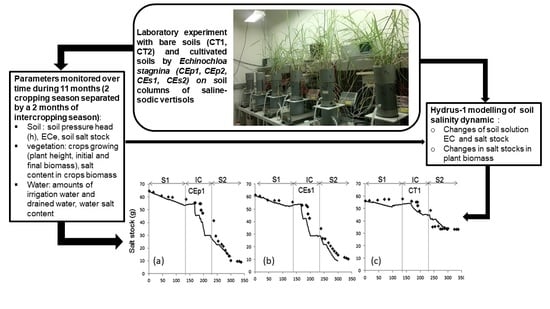
The simulated SS followed the same dynamics as ECe and agreed with the measurements from all columns (Figure 5), with a low RMSE (0.3–4.0 g) and high NSE (0.70–0.99). Simulated and measured results showed that the soil SS, initially the same among treatments (Figure 5), decreased for most of the experiment. At the end of the first cropping season, the SS had decreased by 5–14% in soil cultivated with E. stagnina (CEp and CEs), but had increased by 3% in bare soil (CT1 and CT2). The SS decreased more during the intercropping season, when water was periodically ponded on cracked soil. At the end of the intercropping season, the initial SS had decreased by 35–45% in soil cultivated with E. stagnina and by 14–22% in bare soil. At the end of the experiment, the SS was higher in bare soil (33–40 g per column) than in cultivated soils (9–22 g per column).

The salt balance, calculated from the initial soil SS, salt inputs from irrigation water and the final soil SS at the end of the experiment, was positive in all columns, confirming soil desalinization (

Table 5. Soil salt balance established at the end of the experiment between the initial salt stock (SSi), salt supplied by irrigation water (SSe) and the final salt stock (SSf) in the six columns. CT1 and CT2 are the columns with bare soil. CEs1 and CEs2 are the columns cultivated with seasonal E. stagnina and CEp1 and CEp2 are the columns cultivated permanently with E. stagnina.

Component	CEp1	CEp2	CEs1	CEs2	CT1	CT2
SSi	64.5	59.0	61.3	57.2	56.2	58.3
SSe	7.6	7.9	7.7	7.1	4.4	3.4
SSf	9.2	20.3	10.4	22.2	33.1	40.5
∆SS	63.0	46.6	58.7	42.1	27.4	21.2
Desalinization %	87	70	85	65	45	34

). Irrigation water contributed to 11–13% of the soil SS (i.e., 7.1–7.9 g per column) in columns cultivated with E. stagnina and to 6–8% of the soil SS (i.e., 3.4–4.4 g per column) in bare soil, due to the larger amount of irrigation water in columns cultivated with E. stagnina. At the end of the experiment, the SS had decreased more in soil cultivated with E. stagnina (by 65–87%) than in bare soil (by 34–45%).

3.5. Dynamics of Salt Stock during the Intercropping Season

Periodic water ponding during the intercropping season decreased the soil SS in cracked soil in all columns (Figure 6). Although all columns received the same amount of water, more salt was removed from soil cultivated with E. stagnina (17–21 g per column) than from bare soil (10–15 g per column). At the end of the intercropping season, ponding in soil cultivated with E. stagnina had removed 31–39% of the soil SS present at the beginning of the intercropping season (i.e., 30–36% of initial SS in the columns). In contrast, ponding in bare soil had removed 17–25% of the soil SS present at the beginning of the intercropping season (i.e., 18–26% of initial soil SS).

4. Discussion

4.1. E. stagnina as a Crop for Effectively Decreasing the Salinity of Vertic Soils

This study shows that the fodder crop of E. stagnina reduces soil salinity of saline-sodic Vertisols. Indeed, after 15 months of growth on soil columns under laboratory conditions, the SS decreased considerably in soils cultivated with E. stagnina (65–87%) while it only decreased by 34–45% in submerged bare soil. The same tendency was also observed with the EC reduction which was more pronounced in soil cultivated by E. stagnina than in submerged bare soil, particularly in deeper layers.

At the end of the experiment, the initially saline soils had become non-saline (ECe < 4 dS/m). These results confirm the ability of E. stagnina to decrease soil salinity, as reported by previous studies [12,15,32]. Ref. [15] reported similar percentages of soil desalinization under field conditions, observing that E. stagnina grown in saline Vertisols reduced the SS by 72–81% in the topsoil (0–10 cm) after 8 months of field growth in the Niger River valley. This decrease was similar to that of [12], who observed that E. stagnina grown for two years on a saline-sodic clay soil in Egypt reduced the soil ECe significantly (from 27.6 to 4.3 dS/m) in the 0–15 cm soil layer. These two studies were conducted under field conditions, while our laboratory conditions allowed for measurement of ECe at three depths and with drainage at the bottom of the columns. Pot experiments of vertic soil planted with Lotus corniculatus without drainage also experienced a decrease in ECe (from 8.37 to 2.11 dS/m) after 2 months of growth [53]. Several other studies have shown the impacts of salt-tolerant plants or halophytes to reduce soil salinity, such as Suadea maritima, Sesuvium potulacastrum and Ipomoea pers-caprae by [9], Lonicera japonica by [54], or Atriplex aucheri, Suaeda salsa and Salicornia europea by [41].

The reduction in soil salinity by E. stagnina is explained mainly by (i) its root system improving soil structure with a higher soil macroporosity, (6–9%) in comparison to bare soil (3–4%) as reported by [35], and increasing salt leaching which is the dominant process and (ii) by salt accumulation in plant biomass [15,32,41]. The relative importance of these two processes has also been reported by [16].

4.2. Modeling of Vertisol Soil Salinity Phytoreclamation by HYDRUS-1D

The Hydrus-1D model allowed simulation of the general trends in the phytodesalinization processes of Vertisols by the E. stagnina crop. Indeed, the simulated results agreed with the measurements, highlighting a decrease of the soil ECw and SS in soil cultivated with E. stagnina. At the end of the experiment, simulations and measurements showed that ECw and SS were greater in bare soil than in soil cultivated with E. stagnina. However, the simulations were performed without considering geochemical processes (e.g., salt dissolution or precipitation), which may have biased model predictions. Although model predictions followed the general trends of salt accumulation measured in plant biomass, the model predicted less salt in plant biomass, particularly during the second cropping season. Based on the threshold in the simulated salt accumulation predicted at the beginning of the second cropping season (Figure 5), we assume that the prediction of water uptake and consequently salt uptake was the main source of uncertainty. The salinity stress threshold in the [51] function was calibrated for a plant (ryegrass) that does not necessarily have the same agronomic characteristics as E. stagnina.

Refs. [27,28] used Hydrus-1D to simulate the effects of gypsum amendment on soil salinity dynamics in a saline-sodic clay soil. Their predictions agreed with the measurements, showing a decrease in soil ECe in saline-sodic clay soil after gypsum application. Recently, ref. [29] coupled Hydrus-1D with the UNSATCHEM module to simulate the Ca, Na, Mg and K contents of sodic Vertisols reclaimed with gypsum amendment and irrigated with water of varying quality. Unlike our study, these studies excluded plant effects from the simulations, particularly the salt accumulation in plant biomass. We simulated soil with a single-porosity model during the cropping seasons and a double-porosity model during the intercropping season, assuming that the hydraulic parameters changed over time but were constant during each season. However, these hydraulic parameters may change progressively, given the shrink–swell processes of Vertisols [25,26,55]. These variations in the hydraulic parameters of Vertisols may affect soil desalinization, but they remain difficult to assess in our modeling approach. Moreover, other simulation models have been developed to consider geochemical processes (e.g., salt dissolution and precipitation). For example, PHREEQ-C [56] and SWAP [57] simulate both the salt accumulation in plant biomass based on plant growth and salt leaching based on the improvement in soil structure due to plant root systems.

4.3. Role of the Intercropping Season in the Desalinization of Vertisols

Soil cultivated with E. stagnina cracks more than bare soil, highlighting the benefits of E. stagnina roots, as reported by many authors [58,59]. Moreover, the intercropping season promotes soil restructuring during soil cracking, due to shrinkage mechanisms during the drying phase. The periodic water ponding on cracked soil during the intercropping season induced water flow bypass and salt transfer between the soil matrix and the macroporosity induced by cracks. The total amount of salt removed during the intercropping season by water ponding represented 30–36% of the initial SS in soil cultivated with E. stagnina and 18–26% of the initial SS in bare soil. Several authors [15,60,61,62] also reported these processes, explaining that during the intercropping season, salt in cracked clay soils moves from the inside to the outside of soil prisms (due to evaporation), precipitates on prism faces and then becomes easily dissolved and leached by irrigation. However, ref. [63] reported that water flow bypass in cracks limits salt dissolution in the soil matrix, questioning the effectiveness of soil desalinization by water ponding on cracked soil. Moreover, supplying water causes early crack closure (4–5 h) in Vertisols [61,64] and low saturated hydraulic conductivity (2.8 × 10⁻⁸ m/s), which decreases water infiltration and salt leaching [4,15]. The financial cost of moving water during this period without crop production may also limit the feasibility of this technique, particularly under arid and semi-arid conditions.

5. Conclusions

This study showed that the E. stagnina crop reduced the soil salinity of Vertisols and the Hydrus-1D model allowed simulation of the general trends in the phytodesalinization processes of Vertisols. Indeed after 11 months of growth, simulated and measured results showed that the SS, which was initially the same in all columns, decreased by 65–87% in soil cultivated with E. stagnina and by 34–45% in ponded bare soil. However, the simulated salt accumulation in plant biomass was lower than that measured, with a pronounced difference from the beginning of the second cropping season. Our results suggested that planting E. stagnina is a promising option for reducing the soil salinity of saline-sodic Vertisols. A simplified modeling approach based on Hydrus-1D was adequate for predicting the general dynamics of soil salinity. The fodder crop of E. stagnina can improve irrigated salt-affected lands and improve cropping systems by the diversification of agricultural production of irrigated land.

References

- Shrivastav, P.; Kumar, R. Soil salinity: A serious environmental issue and plant growth promoting bacteria as one of the tools for its alleviation. Saudi J. Biol. Sci. 2015, 22, 123–131. [Google Scholar] [CrossRef] [Green Version]
- Jamil, A.; Riaz, S.; Ashraf, M.; Foolad, M.R. Gene expression profiling of plants under salt stress. Crit. Rev. Plant Sci. 2011, 30, 435–458. [Google Scholar] [CrossRef]
- Balpande, S.S.; Deshpande, S.B.; Pal, D.K. Factors and processes of soil degradation in Vertisols of the Purna Valley, Maharashira, India. Land Degrad. Dev. 1996, 7, 313–324. [Google Scholar] [CrossRef]
- Adam, I.; Michot, D.; Guero, Y.; Soubega, B.; Moussa, I.; Walter, C. Detecting soil salinity changes in irrigated Vertisols by electrical resistivity prospection during a desalinization experiment. Agric. Water Manag. 2012, 109, 1–10. [Google Scholar] [CrossRef]
- Guéro, Y. Contribution à L’étude des Mécanismes de Dégradation Physico-Chimique des Sols Sous Climat Sahélien. Exemple Pris dans la Vallée du Moyen Niger. Ph.D. Thesis, Université Abdou Moumouni, Niamey, Niger, 2000; p. 109. [Google Scholar]
- Adam, I. Cartographie Fine et Suivi Détaillé de la Salinité des Sols d’un Périmètre Irrigué au Niger en Vue de Leur Remédiation. Ph.D. Thesis, Université Abdou Moumouni, Rennes, France, 2011; p. 219. [Google Scholar]
- Nouri, H.; Borujeni, S.C.; Nirola, R.; Hassanli, A.; Beecham, S.; Alaghmand, S.; Saint, C.; Mulcahy, D. Application of green remediation on soil salinity treatment: A review on halophytoremediation. Process Saf. Environ. Prot. 2017, 107, 94–107. [Google Scholar] [CrossRef]
- Qadir, M.; Ghafoor, A.; Murtaza, G. Amelioration strategies for saline soils: A review. Land Degrad. Dev. 2000, 11, 501–521. [Google Scholar] [CrossRef]
- Ravindran, K.C.; Venkatesan, K.; Balakrishnan, V.; Chellappan, K.P.; Balasubramanian, T. Restoration of saline land by halophytes for Indian soils. Soil Biol. Biochem. 2007, 39, 2661–2664. [Google Scholar] [CrossRef]
- Zorrig, W.R.M.; Ferchichi, S.; Smaoui, A.; Abdelly, C. Phytodesalination: A solution for salt-affected soils in arid and semi-arid regions. J. Arid Land Stud. 2012, 22, 299–302. [Google Scholar]
- Jesus, J.M.; Danko, A.S.; Fiúza, A.; Borges, M.T. Phytoremediation of salt-affected soils: A review of processes, applicability, and the impact of climate change. Environ. Sci. Pollut. Res. 2015, 22, 6511–6525. [Google Scholar] [CrossRef] [PubMed]
- Helalia, A.M.; El-Amir, S.; Abou-Zeid, S.T.; Zaghloul, K.F. Bio-reclamation of saline-sodic soil by Amshot grass in Northern Egypt. Soil Tillage Res. 1992, 22, 109–115. [Google Scholar] [CrossRef]
- Qadir, M.; Qureshi, R.H.; Ahmad, N.; Ilyas, M. Saline-sodic field for biomass production and soil reclamation salt-tolerant forage cultivation. Land Degrad. Dev. 1996, 7, 11–18. [Google Scholar] [CrossRef]
- Rabhi, M.; Karray-Bouraoui, N.; Medini, R.; Attia, H.; Athar, H.U.R.; Abdelly, C.; Smaoui, A. Seasonal variations in phytodesalination capacity of two perennial halophytes in their natural biotope. J. Biol. Res.-Thessalon. 2010, 14, 181–189. [Google Scholar]
- Ado, M.N.; Guéro, Y.; Michot, D.; Soubeiga, B.; Senga Kiesse, T.; Walter, C. Phytodesalinization of irrigated saline Vertisols in the Niger Valley by Echinochloa stagnina. Agric. Water Manag. 2016, 177, 229–240. [Google Scholar] [CrossRef]
- Qadir, M.; Steffens, D.; Yan, F.; Schubert, S. Sodium removal from a calcareous saline-sodic soil through leaching and plant uptake during phytoremediation. Land Degrad. Dev. 2003, 14, 301–307. [Google Scholar] [CrossRef]
- Ammari, T.G.; Tahboub, A.B.; Saoub, H.M.; Hattar, B.I.; Al-Zubi, Y.A. Salt removal efficiency as influenced by phyto-amelioration of salt-affected soils. J. Food Agric. Environ. 2008, 6, 456–460. [Google Scholar]
- Rabhi, M.; Lakhdar, A.; Hajji, S.; Barhoumi, Z.; Hamrouni, M.H.; Abdelly, C.; Smaoui, A. Evaluation of the capacity of three halophytes to desalinize their rhizosphere as grown on saline soils under nonleaching conditions. Afr. J. Ecol. 2009, 47, 463–468. [Google Scholar] [CrossRef]
- Ahmad, N.; Qureshi, R.H.; Qadir, M. Amelioration of a calcareous saline-sodic soil by gypsum and forage plants. Land Degrad. Rehabil. 1990, 2, 277–284. [Google Scholar] [CrossRef]
- Tanton, T.W.; Rycroft, D.W.; Hashimi, M. Leaching of salt from heavy clay subsoil under simulated rainfall conditions. Agric. Water Manag. 1995, 27, 321–329. [Google Scholar] [CrossRef]
- Qadir, M.; Oster, J.D.; Schubert, S.; Noble, A.D.; Sahrawat, K.L. Phytoremediation of sodic and saline-sodic soils. Adv. Agron. 2007, 96, 197–247. [Google Scholar]
- Jones, C.A. Effect of soil texture on critical bulk densities for root growth. Soil Sci. Soc. Am. J. 1983, 47, 1208–1211. [Google Scholar] [CrossRef]
- Hammecker, C.; Antonino, A.; Maeght, J.L.; Boivin, P. Experimental and numerical study of water flow in soil under irrigation in Northern Senegal: Evidence of air entrapment. Eur. J. Soil Sci. 2003, 54, 491–503. [Google Scholar] [CrossRef]
- Ndiaye, B.; Molénat, J.; Ndoye, S.; Boivin, P.; Cheverry, C.; Gascuel-Odoux, C. Modélisation du transfert de l’eau et des sels dans les casiers rizicoles du delta du fleuve Sénégal. Rev. Sci. L’Eau 2008, 21, 325–336. [Google Scholar] [CrossRef] [Green Version]
- Coppola, A.; Gerke, H.H.; Comegna, A.; Basile, A.; Comegna, V. Dual-permeability model for flow in shrinking soil with dominant horizontal deformation. Water Resour. Res. 2012, 48, 1–21. [Google Scholar] [CrossRef]
- Stewart, R.D.; Abou Najm, M.R.; Rupp, D.E.; Selker, J.S. Modeling multidomain hydraulic properties of shrink-swell soils. Water Resour. Res. 2016, 52, 7911–7930. [Google Scholar] [CrossRef]
- Wang, J.; Bai, Z.; Yang, P. Using HYDRUS to simulate the dynamic changes of Ca2+ and Na+ in sodic soils reclaimed by gypsum. Soil Water Res. 2016, 11, 1–10. [Google Scholar] [CrossRef] [Green Version]
- Reading, L.P.; Baumgartl, T.; Bristow, K.L.; Lockington, D.A. Applying HYDRUS to flow in a sodic clay soil with solution composition–dependent hydraulic conductivity. Vadose Zone J. 2012, 11, vzj2011.0137. [Google Scholar] [CrossRef]
- Mosley, L.M.; Cook, F.; Fitzpatrick, R. Field trial modelling of different strategies for remediation of soil salinity and sodicity in lower Murray irrigation areas. Soil Res. 2017, 55, 670–681. [Google Scholar] [CrossRef]
- Barbiéro, L. Les Sols Alcalinisés sur Socle dans la Vallée du Fleuve Niger. Origines de L’Alcalinisation et Evolution des Sols Sous Irrigation. Ph.D. Thesis, ENSA de Rennes, Rennes, France, 1995. [Google Scholar]
- Léauthaud, H.C. De L’influence des Crues sur les Services Ecosystémiques des Prairies Inondables. Application à la Production Fourragère dans le Delta du Fleuve Tana, au Kenya. Ph.D. Thesis, Université de Montpellier II, Montpellier, France, 2013. [Google Scholar]
- Barbiero, L.; Valles, V.; Régeard, A.; Cheverry, C. Residual alkalinity as tracer to estimate the changes induced by forage cultivation in a non-saline irrigated sodic soil. Agric. Water Manag. 2001, 50, 229–241. [Google Scholar] [CrossRef] [Green Version]
- FAO. World Reference Base for Soil Resources: International Soil Classification System for Naming Soils and Creating Legends for Soil Maps; FAO: Rome, Italy, 2014; p. 192. [Google Scholar]
- Blackwell, P.S.; Jayawardane, N.S.; Green, T.W.; Wood, J.T.; Blackwell, J.; Beatty, H.J. Subsoil macropore space of a transitional red-brown earth after either deep tillage, gypsum or both 1. Physical effects and short-term changes. Aust. J. Soil Res. 1991, 29, 123–140. [Google Scholar] [CrossRef]
- Ado, M.N.; Michot, D.; Guero, Y.; Hallaire, V.; Dan Lamso, N.; Dutin, G.; Walter, C. Echinochloa stagnina improves soil structure and phytodesalinization of irrigated saline sodic Vertisols. Plant Soil 2019, 434, 413–424. [Google Scholar] [CrossRef]
- AFNOR. Détermination de la conductivité électrique spécifique. In Qualité des Sols, Recueil de Normes Françaises, 3rd ed.; Norme NF ISO 11265; AFNOR Editions: Paris-La, Défense, 1996; pp. 521–524. [Google Scholar]
- Slavich, P.G.; Petterson, G.H. Estimating the electrical conductivity of saturated paste extracts from 1:5 soil: Water suspensions and texture. Aust. J. Soil Res. 1993, 31, 73–81. [Google Scholar] [CrossRef]
- Paine, C.E.; Marthews, T.R.; Vogt, D.R.; Purves, D.; Rees, M.; Hector, A.; Turnbull, L.A. How to fit nonlinear plant growth models and calculate growth rates: An update for ecologists. Methods Ecol. Evol. 2012, 3, 245–256. [Google Scholar] [CrossRef]
- Chessel, D.; Dufour, A.B. Modèles Logistiques, Rapport Utilisant le Logiciel R; Université de Lyon1: Lyon, France, 2008; p. 9. [Google Scholar]
- Pinheiro, J.; Bates, D.; DebRoy, S.; Sarkar, D. Nlme: Linear and Nonlinear Mixed Effects Models, R Package Version 3; 2009; pp. 1–86. Available online: https://www.researchgate.net/publication/272475067_The_Nlme_Package_Linear_and_Nonlinear_Mixed_Effects_Models_R_Version_3 (accessed on 29 December 2021).
- Zhao, Z.Y.; Zhang, K.; Wang, P.; Wang, L.; Yin, C.H.; Tian, C.Y. The effects of halophytes on salt balance in an arid irrigation district. J. Food Agric. Environ. 2013, 11, 2669–2673. [Google Scholar]
- Simunek, J.; Sejna, M.; Saito, H.; Sakai, M.; van Genuchten, M.T. The HYDRUS-1D Software Package for Simulating the Movement of Water, Heat, and Multiple Solutes in Variably Saturated Media. Version 4.0; Hydrus Software; Department of Environmental Sciences University of California Riverside: Riverside, CA, USA, 2008; p. 315. [Google Scholar]
- Vanderboght, J.; Vereecken, H. Review of dispersivities for transport modelling in soils. Vadose Zone J. 2007, 6, 29–52. [Google Scholar] [CrossRef]
- Mualem, Y. A new model for predicting the hydraulic conductivity of unsaturated porous media. Water Resour. Res. 1976, 12, 513–522. [Google Scholar] [CrossRef] [Green Version]
- Van Genuchten, M.T. A closed-form equation for predicting the hydraulic conductivity of unsaturated soils. Soil Sci. Soc. Am. J. 1980, 44, 892–898. [Google Scholar] [CrossRef] [Green Version]
- Schaap, M.G.; Leij, F.J.; van Genuchten, M.T.; Rosetta, M.T. A computer program for estimating soil hydraulic parameters with hierarchical pedotransfer functions. J. Hydrol. 2001, 251, 163–176. [Google Scholar] [CrossRef]
- Gerke, H.H.; van Genuchten, M.T. A dual-porosity model for simulating the preferential movement of water and solutes in structured porous media. Water Resour. Res. 1993, 29, 305–319. [Google Scholar] [CrossRef]
- Skaggs, T.H.; van Genuchten, M.T.; Shouse, P.J.; Poss, J.A. Macroscopic approaches to root water uptake as a function of water and salinity stress. Agric. Water Manag. 2006, 86, 140–149. [Google Scholar] [CrossRef]
- Phogat, V.; Skewes, M.A.; Cox, J.W.; Sanderson, G.; Alam, J.; Simunek, J. Seasonal simulation of water, salinity and nitrate dynamics under drip irrigated mandarin (Citrus reticulata) and assessing management options for drainage and nitrate leaching. J. Hydrol. 2014, 513, 504–516. [Google Scholar] [CrossRef] [Green Version]
- Feddes, R.A.; Kowalik, P.J.; Zaradny, H.X. Simulation of Field Water Use and Crop Yield; Centre for Agricultural Publishing and Documentation: Wageningen, The Netherlands, 1982; pp. 194–209. [Google Scholar]
- Maas, E.V. Crop salt tolerance. In Agricultural Salinity Assessment and Management; Tanji, K.K., Ed.; ASCE Manuals and Reports on Engineering Practice, No 71; ASCE Press: New York, NY, USA, 1990. [Google Scholar]
- Simunek, J.; Hopmans, J.W. Modeling compensated root water and nutrient uptake. Ecol. Model. 2009, 220, 505–521. [Google Scholar] [CrossRef]
- Aydemir, S.; Sünger, H. Bioreclamation effect and growth of a leguminous forage plant (Lotus corniculatus) in calcareous saline-sodic soil. Afr. J. Biotechnol. 2011, 10, 15571–15577. [Google Scholar] [CrossRef]
- Yan, K.; Xu, H.; Zhao, S.; Shan, J.; Chen, X. Saline soil desalination by honeysuckle (Lonicera japonica Thunb.) depends on salt resistance mechanism. Ecol. Eng. 2016, 88, 226–231. [Google Scholar] [CrossRef]
- Garnier, P.; Perrier, E.; Bellier, G.; Rieu, M. Modelling water flow in unsaturated swelling soil samples. Bull. Soc. Geol. Fr. 1998, 169, 589–593. [Google Scholar]
- Parkhurst, D.L.; Appelo, C.A.J. Description of Input and Examples for PHREEQC Version 3: A Computer Program for Speciation, Batch-Reaction, One-Dimensional Transport, and Inverse Geochemical Calculations; U.S. Geological Survey: Menlo Park, CA, USA, 2013; p. 497. [Google Scholar]
- Kroes, J.; Van Dam, J.C.; Groenendijk, P.; Hendriks, R.F.A.; Jacobs, C.M.J. SWAP Version 3.2: Theory Description and User Manual; Alterra: Wageningen, The Netherlands, 2009; p. 262. [Google Scholar]
- Mitchell, A.R.; Ellsworth, T.R.; Meek, B.D. Effect of root systems on preferential flow in swelling soil. Commun. Soil Sci. Plant Anal. 1995, 26, 2655–2666. [Google Scholar] [CrossRef]
- Angers, D.A.; Caron, J. Plant-induced changes in soil structure: Processes and feedbacks. Biogeochemistry 1998, 42, 55–72. [Google Scholar] [CrossRef]
- Wallender, W.W.; Tanji, K.K.; Gilley, J.R.; Hill, R.W.; Lord, J.M.; Moore, C.V.; Robinson, R.R.; Stegman, E.C. Water flow and salt transport in cracking clay soils of the Imperial Valley, California. Irrig. Drain. Syst. 2006, 20, 361–387. [Google Scholar] [CrossRef]
- Favre, F.; Boivin, P.; Wopereis, M. Water movement and soil swelling in a dry, cracked Vertisols. Geoderma 1997, 78, 113–123. [Google Scholar] [CrossRef]
- Maruyama, T.; Tanji, K.K. Physical and Chemical Processes of Soil Related to Paddy Drainage; Shinzan-Sha Science and Technology: Tokyo, Japan, 1997; p. 229. [Google Scholar]
- Bouma, J. Field measurement of soil hydraulic conductivity characterizing water movement through swelling clay soils. J. Hydrol. 1980, 45, 149–158. [Google Scholar] [CrossRef]
- Greve, A.; Andersen, M.S.; Acworth, R.I. Investigations of soil cracking and preferential flow in a weighing lysimeter filled with cracking clay soil. J. Hydrol. 2010, 393, 105–113. [Google Scholar] [CrossRef]
Figure 1.
Design of Echinochloa stagnina growth experiment on reconstituted saline Vertisols.
Figure 2.
Dynamics of the pressure head (h) measured with tensiometers (M) and simulated with Hydrus−1D (S) at 5, 15 and 21 cm soil depths in soil columns for the three treatments during the experiment. S1 is the first cropping season, IC is the intercropping season, S2 is the second cropping season, CEp1 (a) and CEp2 (b) are the columns cultivated permanently with E. stagnina, CEs1 (c) and CEs2 (d) are the columns cultivated with seasonal E. stagnina, and CT1 (e) and CT2 (f) are the columns with bare soil.
Figure 3.
Dynamics of electrical conductivity (ECw) measured in soil solution (M) and simulated with Hydrus-1D (S) at 5, 15 and 21 cm soil depths in soil columns for the three treatments during the experiment. S1 is the first cropping season, IC is the intercropping season, S2 is the second cropping season, CEp1 (a) and CEp2 (b) are the columns cultivated permanently with E. stagnina, CEs1 (c) and CEs2 (d) are the columns cultivated with seasonal E. stagnina, and CT1 (e) and CT2 (f) are the columns with bare soil.
Figure 4.
Dynamics of salt accumulation in plant biomass of E. stagnina measured in dry shoot and root biomass (M) and simulated with HYDRUS-1D (S) for the three treatments during the experiment. S1 is the first cropping season, IC is the intercropping season, S2 is the second cropping season, CT1 and CT2 are the columns with bare soil, CEp1 (a) and CEp2 (b) are the columns cultivated permanently with E. stagnina, CEs1 (c) and CEs2 (d) are the columns cultivated with seasonal E. stagnina.
Figure 5.
Dynamics of soil salt stock calculated in dry soil mass (M) and simulated (S) for the three treatments during the experiment. S1 is the first cropping season, IC is the intercropping season, S2 is the second cropping season, CEp1(a) and CEp2 (b) are the columns cultivated permanently with E. stagnina, CEs1 (c) and CEs2 (d) are the soil columns cultivated with seasonal E. stagnina, CT1 (e) and CT2 (f) are the columns with bare soil.
Figure 6.
Relationship between cumulative irrigation and the soil salt stock in soil columns for the three treatments during the intercropping season. CEp1 and CEp2 are the columns cultivated permanently with E. stagnina, CEs1 and CEs2 are the columns cultivated with seasonal E. stagnina, CT1 and CT2 are the columns with bare soil.