Article

Impact of Drought and Changing Water Sources on Water Use and Soil Salinity of Almond and Pistachio Orchards: 2. Modeling

1
Department of Environmental Sciences, University of California Riverside, Riverside, CA 92521, USA
2
USDA-Agricultural Research Service, US Salinity Laboratory, Agricultural Water Efficiency and Salinity Research Unit, Riverside, CA 92507, USA
*
Authors to whom correspondence should be addressed.
Soil Syst. 2021, 5(4), 58; https://doi.org/10.3390/soilsystems5040058
Submission received: 10 May 2021 / Revised: 16 July 2021 / Accepted: 10 September 2021 / Published: 24 September 2021
(This article belongs to the Special Issue Advances in the Prediction and Remediation of Soil Salinization)

Abstract

:
California is increasingly experiencing drought conditions that restrict irrigation deliveries to perennial nut crops such as almonds and pistachios. During drought, poorer quality groundwater is often used to maintain these crops, but this use often results in secondary salinization that requires skilled management. Process-based models can help improve management guidelines under these challenging circumstances. The main objective of this work was to assess seasonal soil salinity and root water uptake as a function of irrigation water salinity and annual rain amounts. The manuscript presents a comparison of three-year experimental and numerically simulated root zone salinities in and below the root zone of almond and pistachio drip-irrigated orchards at multiple locations in the San Joaquin Valley (SJV), California, with different meteorological characteristics. The HYDRUS-1D numerical model was calibrated and validated using field measurements of soil water contents and soil solute bulk electrical conductivities at four root zone depths and measured soil hydraulic conductivities. The remaining soil hydraulic parameters were estimated inversely. Observations and simulations showed that the effects of rain on root zone salinity were higher in fields with initially low salinities than in fields with high salinities. The maximum reduction in simulated root water uptake (7%) occurred in response to initially high soil salinity conditions and saline irrigation water. The minimum reduction in simulated water uptake (2.5%) occurred in response to initially low soil salinity conditions and a wet rain year. Simulated water uptake reductions and leaching fractions varied at early and late times of the growing season, depending on irrigation water salinity. Root water uptake reduction was highly correlated with the cumulative effects of using saline waters in prior years, more than salt leaching during a particular season, even when rain was sufficient to leach salts during a wet year.

1. Introduction

California’s agricultural management practices need to be adjusted to account for ongoing water scarcity and forecasted climate change. It is essential to quantify and predict management effects on soil properties and model their consequent impacts on production and the environment [1]. Developing sustainable agricultural practices requires using methods that accurately describe salinity patterns and changes in salinity over time and space [2]. A comprehensive understanding of the spatial distribution of deep percolation fluxes due to the spatial distribution of soil properties and spatial vegetation heterogeneities is still needed to develop such strategies [3].
Soil salinity, similarly to soil water content, is often variable in time and space. A complete analysis of transient salt transport in the root zone requires extensive measurements, a long time, and significant efforts and costs. On the other hand, numerical models have proven to be valuable and efficient tools for carrying out spatial-temporal agricultural system analyses aimed at enhancing productivity under various irrigation schemes and assessing ongoing climate change effects on soil salinity [4,5,6,7]. In particular, transient-state salinity models are desirable for the analysis of management [8]. Soil salinity problems integrate the effects of many time-varying factors, including soil properties, climate, crops, irrigation methods, and management practices. Therefore, transient models can provide solutions for quantifying salinity build-up in the root zone due to these various processes and factors. These may include irrigation-induced salinity, upward movement of salts from the saline groundwater table, and sodification processes [9].
There is a need to develop practical and straightforward (e.g., quicker and cheaper) methods to determine and evaluate soil salinity to improve decision-making processes and soil salinity stress management [10,11,12]. The accuracy of salinity build-up and water uptake predictions depends on selecting proper mathematical models [13]. Modeling can explain how temporal and spatial aspects of soil water and solute fluxes are affected by irrigation practices [14]. Feddes and Raats [15] summarized the progress, challenges, and applications of unsaturated-zone modeling.
Simulations using transient-state models for actual field conditions require information about the quantity and quality of waters entering the soil (e.g., rainwater and irrigation water), other climate variables (e.g., evapotranspiration), soil hydraulic, and transport properties, and crop properties. The continuous changes that occur throughout the root zone are a function of irrigation water salinity, amounts of applied water, rainfall, crop evapotranspiration (ET), and other climate variables [16]. Gigante et al. [17] stated that vegetation’s space-time distribution is crucial for a correct evaluation of soil evapotranspiration and other components of soil water balance. However, some of the past analyses that compared models used to evaluate steady-state and transient-based leaching requirements ignored rainfall and did not correctly represent field conditions [18].
The HYDRUS-1D model [14] has been used in many studies to assess soil salinity problems, including those involving drip irrigation, through a one-dimensional or two-dimensional analysis [7,19,20,21,22,23,24]. For example, Ramos et al. [22] concluded that HYDRUS-1D is a powerful tool for analyzing solute concentrations related to overall soil salinity and nitrogen species. Haj-Amor et al. [25] used HYDRUS-1D to clarify the impact of different water salinities and irrigation practices on soil salinity (expressed as electric conductivity, EC), which exceeded the palm salt tolerance in their study. Li et al. [4] used HYDRUS-1D to investigate the effects of soil water dynamics, soil salinization, and groundwater salinity. In their research, simulated soil water contents (SWC) and electrical conductivities (ECs) of the soil solution were in suitable agreement with the observations.
The HYDRUS-1D model [14] provides two different approaches to simulate soil salinity in agricultural soils. First, the HYDRUS-1D standard module can simulate overall salinity by assuming that EC behaves as a tracer. Second, the HYDRUS-1D multicomponent major ion chemistry module UNSATCHEM permits simulations that account for multiple geochemical reactions involved in the salinization process, such as precipitation-dissolution of minerals and cation exchange. This is a complex and advanced numerical tool to predict coupled processes of major ion chemistry, variably saturated water flow, and solute transport in soils during transient conditions. The UNSATCHEM module considers the salinization process in its full complexity while considering all major ion interactions. Ramos et al. [22] compared these two modeling approaches and concluded that they provide similar results as long as the effects of geochemical reactions, such as precipitation-dissolution of mineral salts and cation exchange, can be neglected. Additionally, Ramos et al. [26] modeled two-dimensional water flow and nitrogen fate and transport in a sweet sorghum field irrigated with fresh and blended saline waters using HYDRUS-2D.
Models such as HYDRUS generally require extensive calibration to confirm that water flow and solute transport and all boundary conditions of the simulated scenarios are suitably addressed by the model structure [7,12]. Accurate predictions of such models rely on the precise determination of soil hydraulic characteristics [27] or their estimation using pedotransfer function models, such as ROSETTA [28]. The unsaturated soil hydraulic properties are described in the HYDRUS-1D model using the van Genuchten–Mualem hydraulic relations [29]. The pedotransfer functions implemented in the ROSETTA module [28] of HYDRUS-1D use neural networks to predict soil hydraulic parameters from soil texture and related data. The ROSETTA module predicts the following soil hydraulic parameters: the residual water content (θr), the saturated water content (θs), the saturated hydraulic conductivity (Ks), and the fitting parameters n and α of the van Genuchten–Mualem soil hydraulic model [29]. Studies have indicated that the laboratory-measured soil hydraulic parameters, e.g., α, n, and l in the van Genuchten–Mualem functions, combined with pedotransfer functions and inverse optimization algorithms, are effective in simulating soil water contents and salinities [14,30].
In part one of this manuscript series [31], we presented experimental data for several locations in the San Joaquin Valley (hereafter SJV), including precipitation, irrigation, ET fluxes, soil hydraulic properties, and measured root zone soil water contents and electrical conductivities. We also summarized seasonal averages and maximum values of root zone salinity. Periods with maximum values suggest opportunities for improved soil leaching or other management practices.
In this second manuscript, we aim to use the experimental data from selected sites presented in part one [31] to (i) calibrate the HYDRUS-1D numerical model simulating transient root zone deep percolation, and plant water uptake, (ii) relate salt leaching fluxes and accumulated salt concentrations to soil properties, winter rainfall, and irrigation water quantity and quality, and (iii) establish base simulations of root zone salinity for two regions of the San Joaquin Valley (SJV), California. These base simulations and the calibrated model will then be used in a future part 3 of this manuscript series (Helalia et al., in prep.) to evaluate the impacts of likely future climate change scenarios on the sustainability of almond and pistachio orchards agriculture in SJV and to provide management recommendations considering available water resources and their quality to mitigate any negative and adverse impacts of anticipated climate change.

2. Materials and Methods

2.1. Field Sites

A detailed description of five agricultural orchards with five different salinity levels is given in part 1 of this manuscript series. The five sites have eddy covariance towers that are part of the Ameriflux network [32,33,34,35,36]. As shown in Table 1, three sites are on the west side of San Joaquin Valley (SJV), while two sites are on the eastern side. Rainfall on the east side of SJV (about 275 mm/year) is higher than on the western side (about 190 mm/year) due to the rain shadow effect of the coast ranges of California. Two of the west SJV orchards sites are almond, and one is pistachio. On the east side, one is almond, and one is pistachio. Initial salinities, defined as the electrical conductivity of the saturated soil solution extract, averaged over the root zone (about 120 cm deep), are below 2 dS/m at the low salinity sites, about 3 dS/m at the medium salinity site, and above 4 dS/m at the high salinity sites (Table 1). All orchards were irrigated using drip irrigation.
The Sierra Nevada provides surface waters with very low salinity for irrigation in the eastern SJV. When surface water is available for the western SJV, it has increased salinity from passing through the California Delta to the Central Valley Project and State Water Project [37]. Irrigation water salinity at the eastern sites (ASL and PSL) is about 0.04–0.24 dS/m. The western sites were chosen because they were irrigated with saline groundwaters before this study was initiated due to a prolonged historic drought from 2011 to 2016.
Irrigation water samples were collected at different times of the growing season. Five replications are presented for most sites in Table 2. As mentioned in part 1, few samples were available from ASL due to that site’s irrigation strategy. A couple of samples from outside the study period showed ASL to have very low salinity water comparable to PSL, so we assumed that ASL had the same composition as PSL. All measured irrigation water salinity values were used to identify the time-variable concentration boundary conditions. A tipping bucket instrument on the eddy covariance towers (details about various measurements are given in [32]) measured rainfall in each orchard during the 2016–2019 years. Measured rains were compared with rainfall values provided by the California Irrigation Management and Information System (CIMIS) weather stations adjacent to the western and eastern SJV sites. The CIMIS data were very similar to the measured orchard data, which were used in this study’s simulations. In the SJV, seasonal rain events occur mainly from December to March (the winter season). Annual precipitation for a given year tends to be either significantly wetter or drier than the climatological normal. In this study, 2017 was relatively a wet year, and 2018 was a dry year.
The SJV, CA growing seasons for almond and pistachio are given in Table 3. In the analysis below, changes in root zone salinity as affected by winter rains are evaluated based on salinity trends in the “early growing season”. Likewise, the impact of irrigation water quality (Table 2) on soil salinity is based on analyses of “late growing season” salinity trends. Almond has a winter dormancy period between November and January [38], and we define the early growing season to be February to March. The late season is July to August, with harvest in August. Pistachio blooms later than almond, and the early growing season is taken to be April to May, whereas the late season is August to September.

2.2. Model Setup

Simulations of transient soil water flow and solute transport were performed using the HYDRUS-1D model [14,39] for a soil profile 120 cm deep.

2.2.1. Water Flow

The model solves the Richards equation for water flow and the convection-dispersion equation for solute transport in variably saturated porous media numerically. The Richards equation [40] that controls variably saturated water flow is:
θ t = z [ K   ( h z + c o s   α ) ] S
where θ is the soil water content (L3·L−3) t is time (T), z is the vertical space coordinate (L) (positive upward), K is the hydraulic conductivity (L·T−1), h is the pressure head (L), S is the sink term accounting for root water uptake (L3·L−3T−1), and α is the angle between the flow direction and the vertical axis (i.e., α = 0° for vertical flow, α = 90° for horizontal flow, and 0° < α < 90° for inclined flow).
The unsaturated soil hydraulic properties are described using the following van Genuchten–Mualem hydraulic relations [29]:
θ ( h ) { θ r + θ s θ r [ 1 + | α h | n ] m     h < 0 θ s     h 0
K ( h ) = K s K r = K s S e 1 2 [ 1 ( 1 S e 1 m ) ] 2
m = 1 1 n ,   n > 1
S e = θ θ r θ s θ r
where θ r and θ s denote the residual and saturated water contents (L3·L−3 ), respectively, Ks is the saturated hydraulic conductivity (L·T−1), Kr is the relative hydraulic conductivity (-), Se is the effective water content (-), and a (L−1), m (-), and n (-) are empirical parameters in the water retention function.

2.2.2. Initial and Boundary Conditions

The initial root zone soil solute concentrations and water contents were measured at four depths (25, 50, 75, and 100 cm). Atmospheric and free drainage boundary conditions were used at the top and bottom of the soil profile, respectively. The atmospheric variable boundary condition was defined using precipitation, irrigation, and evapotranspiration fluxes as a function of time. Potential evapotranspiration fluxes (ET0) were obtained from the CIMIS meteorological data. Irrigation depths were calculated for each studied orchard using emitter discharges [M3.T−1] and distances between emitters per drip line. Irrigation fluxes were estimated based on seasonal allocations of irrigation provided by the farm managers. Farmers’ estimates of irrigation were adjusted to fulfill the potential evapotranspiration demands (ET0) for almond and pistachio.
In the HYDRUS-1D model, leaf area index (LAI) or surface cover fraction (SCF) of soil by plants are used to estimate potential evaporation (Ep) and potential transpiration (Tp) from potential evapotranspiration (ETp) [14,41,42,43] as shown in Equation (6). The leaf area index values (LAI) and the crop coefficients (Kc) for the studied sites were obtained from satellite NDVI data [44] for 2016–2018. The LAI values were used to estimate the soil cover fractions (SCF) by the canopy at the studied sites (Equation (7)). The SCF was then used to divide potential evapotranspiration ETp into potential evaporation (Ep) and potential transpiration (Tp) using Equations (8) and (9), respectively:
E T P = E T 0 k c
SCF = 1 exp ( r Extinct LAI )
T P = E T P SCF
E P = E T P ( 1 SCF )
where rExtinct is the radiation extinction coefficient (=0.463).

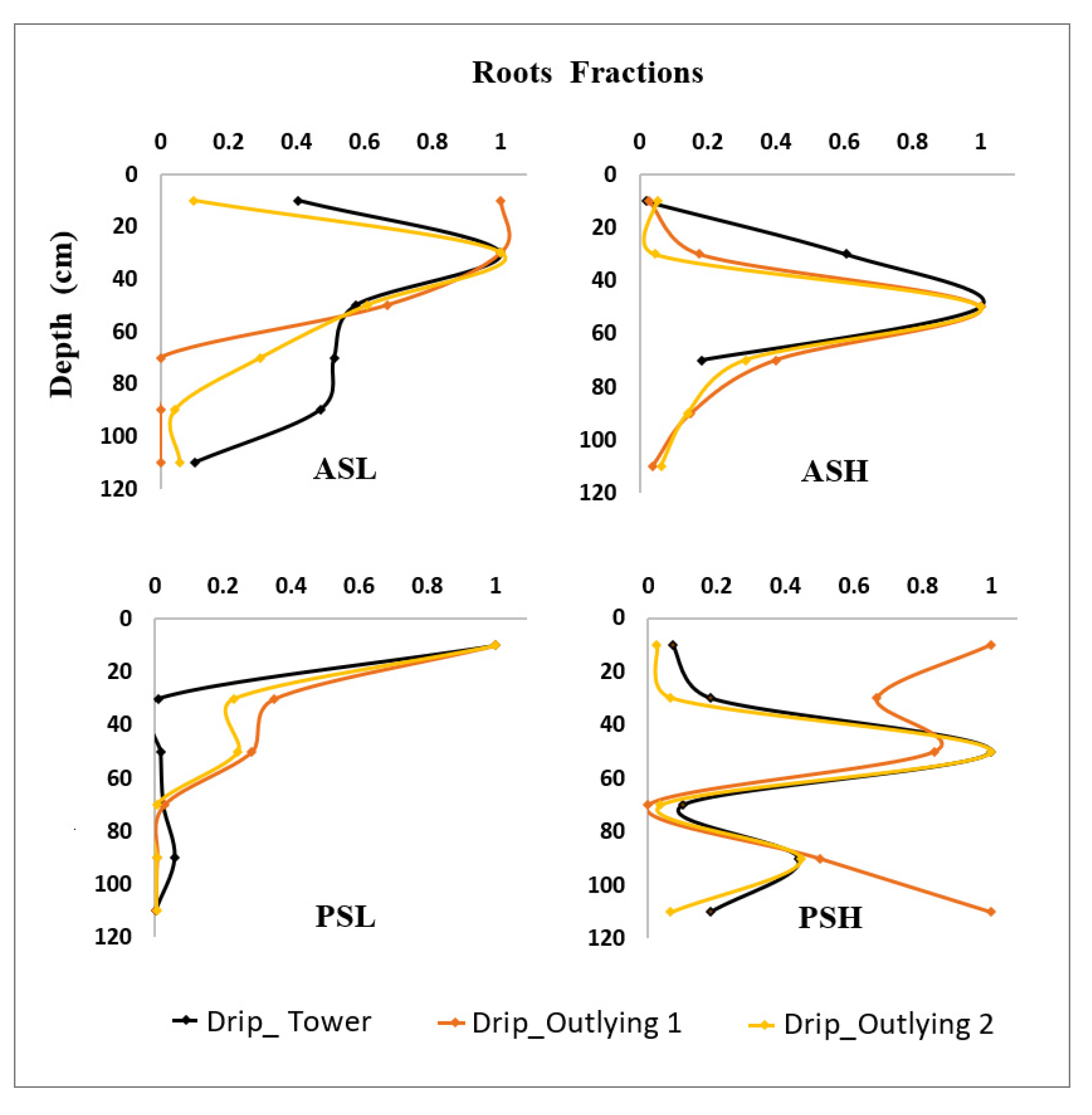
2.2.3. Root Water Uptake

Root water uptake is simulated in HYDRUS-1D using the S-shape model [45]. In this approach, potential transpiration is distributed across the root zone using the root density distribution function to obtain potential root water uptake. This potential uptake is then reduced due to the saturation and salinity stresses represented by corresponding stress response functions [46,47]. The spatial root distribution was determined from measured weights of almond (ASL and ASH) and pistachio (PSL and PSH) roots in six root zone soil layers (Figure 1).
Root water uptake and corresponding yield reductions occur when salts accumulate in the root zone to the extent that the crop cannot extract enough water due to the osmotic (salt) stress. Similarly, root water uptake and yield reductions occur when the soil profile is too dry and there is not enough soil water available for uptake. The root water uptake (transpiration) reduction due to salinity stress is computed in the HYDRUS-1D model using either the threshold and slope function [48] or the S-shape function of van Genuchten [46]. In this research, the S-shape root water uptake model [45] is used to simulate the plant water uptake reduction due to salinity. The root water uptake stress response function parameters of the S-shape function were obtained from the most recent reference values of the salinity reduction slope and threshold values for the studied varieties of almond (Prunus duclis) [48,49,50] and pistachio (Pistacia vera L.) [51].
Crop growth and yield do not respond to salinity until a salinity threshold is reached. Early studies found that almonds have a salinity threshold of 1.8 dS·m−1 [49]. Earlier studies found that pistachios’ (P. vera) shoot growth is reduced at root zone salinity of 7.9 to 10 dS·m−1 [51]. The threshold value for the start of pistachio yield reduction was taken to be 10 dS·m−1, and the 50% reduction was 14–15 dS·m−1 [51].
The parameters of the S-shape model were obtained directly from the threshold and slope model as follows. First, the c50 coefficient (salinity at which the root water uptake reduction is 50%) was calculated as:
c50 = 50/s + cT
where cT is the salinity threshold, and s is the slope of the yield reduction curve. The coefficients of the root water uptake reduction (c50) for almonds and pistachios in this research were calculated as, respectively:
c50 Almond = 50/(19/2) + (1.5 × 2) = 8.263
c50 Pistachio = 50/(10/2) + (5 − 6 × 2) = 20 − 22
The conversion from the EC of the saturated extract (ECe) to the EC of water (ECw) is as follows: ECwke × ECe, where ke is approximately 2 [46]. Consequently, almond and pistachio salinity threshold values were multiplied by the coefficient ke (=2), and the slope values were divided by ke (Equations (11) and (12)).

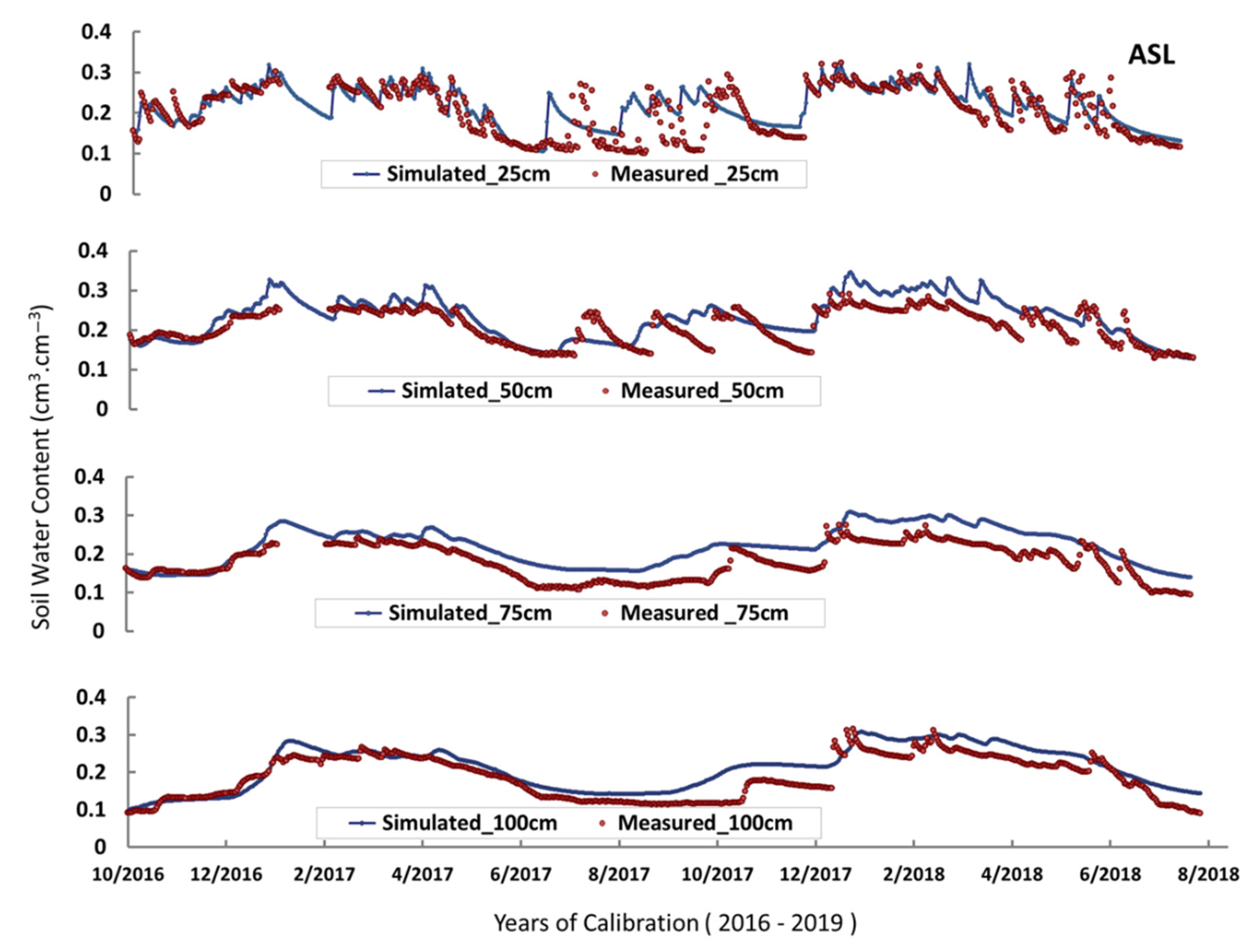
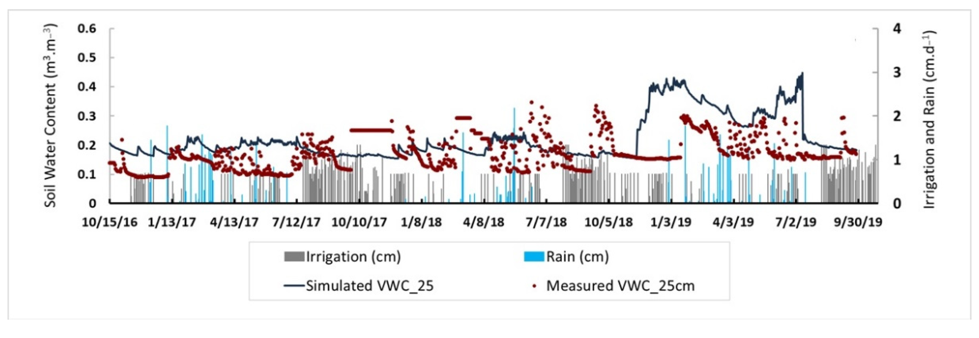
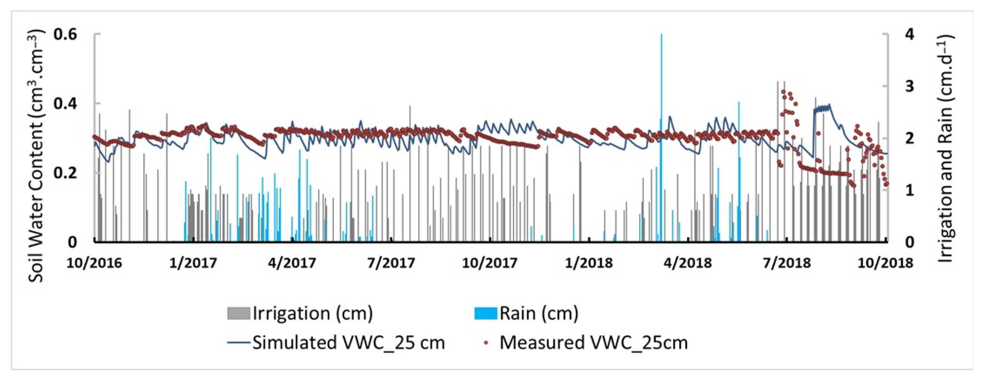
2.3. Model Calibration and Validation

The numerical model was calibrated for the five experimental sites. Soil water contents and soil salinities at depths of 25, 50, 75, and 100 cm measured during 2016–2018 (measurement methods are described in part 1 of this manuscript series [31]) were used in calibration. The model was validated using the third-year data sets from 2018 to 2019.
The HYDRUS-1D codes are physically based models and, as such, require little calibration when all necessary input parameters are experimentally determined. In this study, we measured the saturated soil water content (θs), the average field capacity (θFC) moisture content at 0.33 bar, percentages of sand, silt, and clay, the soil bulk density, and the saturated hydraulic conductivity (Ks). The above-listed soil properties were measured for four layers of each simulated location. The ROSETTA [28] pedotransfer function software was used to predict soil hydraulic parameters θr, α, and n of the soil water retention curve. The measured and ROSETTA-estimated soil hydraulic parameters were used as initial estimates of the soil hydraulic parameters. The inverse optimization option for soil hydraulic parameters implemented in the HYDRUS-1D model was then used to adjust these parameters further to obtain a better correspondence between simulated and measured soil water contents. The obtained soil hydraulic parameters for four depths at five experimental sites are given in Table 4.
The governing convection-dispersion equation for solute transport includes only two parameters when tracer transport is simulated (EC is simulated as a tracer in the standard HYDRUS model). One parameter is the molecular diffusion coefficient, which can be considered using the default HYDRUS value between 1 and 2 cm2/d. The second is the longitudinal dispersivity, which is commonly considered with a value equal to one-tenth of the soil profile depth, i.e., 10 cm. Thus, there are no fitting parameters in the solute transport equation. For calculating the root mean squared error, we used the following formula as shown in Equation (13):
RMSE = 1 N ( y ^ i y obs , i ) 2 N
where RMSE is the root mean squared error, ŷ is the modeled output from HYDRUS, yobs is the observed field value, i is timestep from 1 to N, and N is the length of the time series over which the RMSE is computed.

3. Results

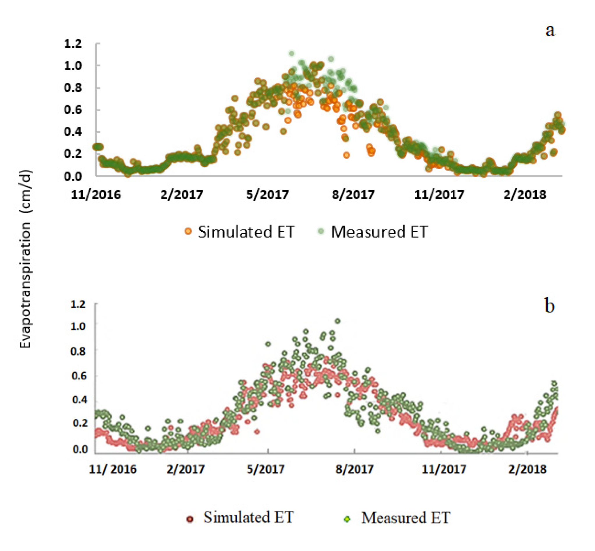
3.1. Root Zone Water Content

Root zone water contents and salinities were analyzed and compared at the five sites. The sites ASL and PSL represent the eastern SJV, and the sites ASH and PSH represent the western SJV.
The effects of rains (mainly in winter) and irrigation on soil water contents in the top root zone at the ASL and ASH sites are shown in Figure 2. The HYDRUS-1D simulated and measured soil water contents (SWCs) showed suitable agreement, both exhibiting time courses that corresponded to rain and irrigation inputs (Figure 2). The seasonal SWC trends show high water contents during the growing season (January–July) due to irrigation and low SWCs during summer. Daily fluctuations in summer were lower at the ASL site (eastern SJV) than at the ASH site (western SJV).
The western site ASH (Figure 2b) had smaller differences in average SWCs between winters and summers than the eastern ASL site (Figure 2a). In summer, the dry and wet events fluctuated more at the ASL site (Figure 2b). In contrast, a long-term stable trend of low SWCs was observed in summer at the ASH site (Figure 2a). The ASH site had a higher soil clay percentage, initial salinity, and SAR than the ASL site (Table 1). The rain total was lower at the ASH site than at the ASL site. Due to these factors, the two regions had a different frequency of topsoil’s wetting and drying patterns. Simulated and measured SWCs at both sites showed an overall high agreement with small values of root mean square errors (RMSEs) at the surface for both sites (Table 5).
At the eastern SJV site ASL, values of simulated and measured SWCs were compared at depths of 25, 50, 75, and 100 cm (Figure 3). The correlation coefficients between the simulated and measured values were 0.91, 0.94, 0.83, and 0.96 at depths of 25, 50, 75, and 100 cm. RMSEs were also low at 0.06 or less (Table 5).
At ASH (Figure 4), the simulated and measured SWCs in the top 25 cm of the root zone showed lower agreement in all seasons, in both wet and dry years of 2017 and 2018, respectively (Table 5). The correlation was highly significant during the winter rain season (October–March), with a p-value of 0.0005. The agreement between simulated and measured SWCs in deeper layers varied depending on the season. In winter (the rainy season), the simulated and measured SWCs showed the highest agreement in the top layer (0–15 cm), with a correlation coefficient of 0.99. The simulated SWCs showed a lower agreement with the measured SWCs at deeper layers, i.e., the correlation coefficients were 0.82 and 0.72 at depths of 75 and 100 cm, respectively. In spring, the highest agreement was obtained in deeper depths of 75 and 100 cm, with correlation coefficients of 0.98 and 0.94, respectively. The correlation was highly significant, as indicated by very low p values (1.5 × 10⁻¹⁹ and 2.7 × 10⁻¹¹). The correlation coefficient for the topsoil layer (25 cm) was 0.62 during the spring (March-May) (Figure 4). These relatively large error values reflect much smaller temporal variations of simulated soil water contents compared to measured ones.
Calibration and validation of the simulated SWCs at depths of 25 for the remaining three sites (of the five studied sites) are presented in Figure 5, Figure 6 and Figure 7. The agreements between measured and simulated water contents were, for various reasons, less suitable at the other three sites than at the ASL and ASH sites (Figure 3 and Figure 4). Irrigation and rainfall at the ASM site (Figure 5) were similar to the ASH site. The ASM site had a layer of clogged semi-permeable dense clay with a measured saturated hydraulic conductivity of only about 0.5 cm/day at a depth of 75 cm. This layer led to the violation of the assumption of one-dimensional flow and transport and poor correspondences between measured and simulated SWCs throughout the soil profile (not shown for other depths). Nevertheless, the RSME for this site was very low (0.078), indicating small errors and high agreement.
The HYDRUS-1D simulated and measured soil water contents (SWCs) at the PSL and PSH sites are shown in Figure 6 and Figure 7, respectively. Surface soil water contents (SWC) at the PSL site (a coarse, well-drained soil) (Figure 6) show much smaller seasonal variations than at the site PSH (a fine soil) (Figure 7). The calibrated model for the PSL site (Figure 6) produced an acceptable agreement between measured and simulated SWCs. Some overestimations occurred during the data validation year (2018–2019). The high saturated hydraulic conductivity of sandy layers above 50 cm, combined with deep, poorly drained duri-pan layers observed at depths of 70–80 cm, hindered the proper validation of HYDRUS-1D for the soil layers above 70 cm (not shown). The root mean square error values for the simulated and measured SWCs were 0.081 and 0.111 at the PSL and PSH sites, respectively.
Finally, the PSH site (Figure 7) has a sodic clay soil, where physicochemical reactions cause slaking of soil aggregates and swelling and dispersion of clay minerals. This leads to a reduction in the soil hydraulic conductivity and a corresponding decrease in infiltration and, hence, the yield. The highest Na concentration measurements were obtained for irrigation waters used at the ASM and PSH sites (Table 2). Additionally, the soils at the ASM and PSH sites have a fine texture and high initial soil solution SAR. The high SAR reduced the soil hydraulic conductivity at both sites (as described in [31]). We believe that the lack of agreement between simulated and measured SWCs at the ASM and PSH sites (Figure 5 and Figure 7) was caused by the previously discussed negative effects of soil SAR on the soil hydraulic conductivity.

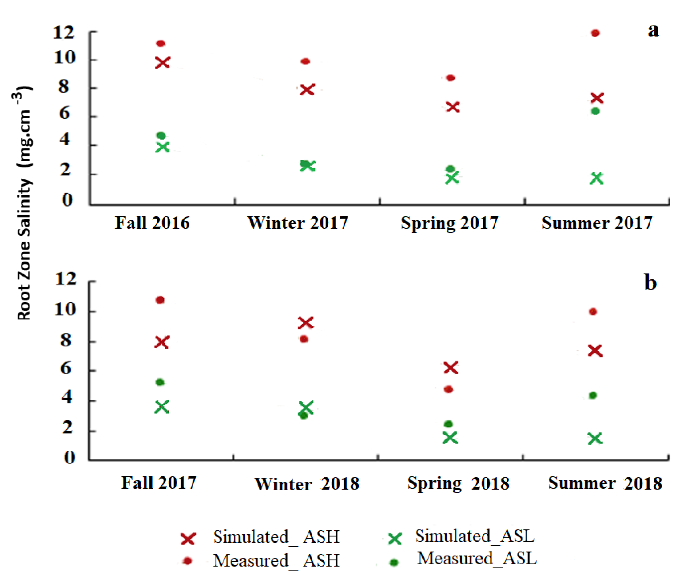
3.2. Root Zone Salinity

Measured and simulated rootzone salinities, i.e., soil water electrical conductivities, are discussed below for the two western and eastern SJV almond sites (for which soil water flow modeling was successful) during two consecutive wet and dry years of 2017 and 2018. The clogged layers at the PSH site and heterogeneous duri-pan layers at the PSL site, with low SWC measurements, prevented HYDRUS-1D from being successfully calibrated against salinities at deeper depths at these two sites. As a result, only the simulations of root zone salinities at the ASL and ASH sites will be used for further analysis.
Salinity increased during the irrigation season (from April to June) at the ASL site in east SJV (Figure 8). During the dry year 2018, soil water salinity reached 6–8 dS·m−1 at depths of 50 and 100 cm, which is marginally higher than almond’s tolerance threshold [48]. During the irrigation season (April to June) of the wet year 2017, rootzone salinity decreased to an average of 2–3 dS·m−1, which is less than half of what was observed in the dry year of 2018. Rain from December to February played a significant role in decreasing root zone salinity to 2–4, 4–6, and 4–6 dS·m−1 at depths of 25, 50, and 100 cm, respectively. The rain reduced the root zone salinities during December and January in all root zone depths in both wet and dry years. The correspondence between simulated and measured root zone salinities and SWCs indicates that HYDRUS-1D can be reliably used to predict future root zone salinity trends at the ASL site.
The correlation coefficients between the measured and simulated salinities were 0.46, 0.59, 0.40, and 0.72 at the root zone depths 25, 50, 75, and 100, respectively. Correlations between measured and simulated salinities were higher in the summer than it in the winter. For example, the correlation coefficients for the deep layers were 0.6 and 0.4 during the summer of 2018 and 2019, respectively, while only 0.2 and 0.4 in the winter. The deep layers showed highly significant correlations in both wet and dry years, with a p-value of 2.7 × 10⁻¹².
We believe that the inability of HYDRUS-1D to produce higher correlations between measurements and simulations of soil salinity was caused by multiple factors. In general, measurement errors, model input errors, and model structure errors could cause disagreement between simulated results and experimental data. First, the distribution of water and salinity is known to be spatially non-uniform when drip emitters are used. The soil water content is highest near the drip line after water application, and then water redistributes throughout the soil profile, as controlled by soil physical properties [52,53]. This non-uniformity could explain deviations between measured and simulated salinities, especially in the shallower depths. Using a two-dimensional version of HYDRUS-1D would likely result in better agreement between experimental and modeled data. Second, while models usually report point values, measurements with suction cups are averaged over a sampling area of a certain volume, the size of which depends on soil hydraulic properties, the soil water content, and the applied suction in the ceramic cup [22,54]. Measured values thus do not represent point values. Third, while measured soil hydraulic parameters were determined in the laboratory on soil samples of a certain size, the obtained parameters may not always represent simulated flow, transport, and reaction processes at a much larger field scale [22]. Forth, while soil hydraulic and solute transport properties are spatially variable at the field scale, our HYDRUS-1D simulations assumed a homogeneous soil environment and thus might not fully account for inherent spatial variability.
Measured salinity increased considerably after the irrigation season (April–July) at the ASH site in the west SJV (Figure 9). Rainfall has a lower effect on reducing root zone salinity at the ASH site, which has a relatively higher initial root zone salinity than the ASL site (Figure 8). The RSME values for the ASH site increased to 1.61, 1.68, and 1.91 dS.m−1 at depths of 25, 50, and 100 cm, respectively.
Simulated and measured concentrations of root zone soil water were averaged over different seasons (spring, summer, fall, and winter) to obtain “seasonal salinities” in terms of electrical conductivities (ECs) as follows:
E C S = Daily   EC Number   of   days   per   season
Simulated and measured data were then grouped for different regions (i.e., the eastern (ASL) and western (ASH) SJV regions) and various seasons (fall, winter, spring, and summer) during both the wet year 2017 (Figure 10a) and the dry year 2018 (Figure 10b). Initial salinity conditions controlled both irrigation and rain effects on increasing and reducing seasonal salinities.
The two data sets are very distinct. Salinities are primarily in the low range of 2–6 dS·m−1 at the ASL site (green lines) and in the high range of 6–12 dS·m−1 at the ASH site (orange lines). The lower range of seasonal salinities in the eastern SJV reflects the effect of the relatively higher mean annual precipitation and higher quality irrigation water. On the other hand, in the western SJV, the higher range of seasonal salinities reflects high soil SAR (Table 1), poorer quality irrigation water, and a low mean annual rainfall. Seasonal salinities were reduced in the middle of the winter seasons in both wet and dry years at both high and low salinity (ASH and ASL, respectively) sites. In the wet year, the effect of rains on reducing soil salinity was higher than the impact of initial salinities.
Simulated and measured seasonal salinities were the highest in the fall and summer of both the wet and dry years of 2017 and 2018, respectively. This increase in soil water salinity reflects the effect of applied irrigation water, in addition to the impacts of initial soil salinity and SAR conditions. The salinity risk at the initially high saline ASH site due to irrigation practices is high. Soil reclamation and amendments to lower initial salinity levels at the beginning of the growing seasons would increase winter rains’ efficiency in reducing root zone salinities and minimizing salinity risk during the irrigation season.
At the ASL site, irrigation water caused only a small increase in seasonal salinities, which remained in an acceptable salinity range. In summer, measured salinity was higher than simulated salinity, which could be related to the irrigation events and dry root zone conditions. The EC measured by GS3 sensors depends on a specific range of soil water contents. When SWCs are less than about 0.10 m3·m−3, the denominator in the pore water conductivity equation for water permittivity becomes very small, leading to significant potential errors [55]. Accordingly, that can lead to the overestimation of measured soil solution electrical conductivities. This would explain some measured values of salinities that were too high when SWCs were lower than 0.10 m3·m−3.
The measured evapotranspiration (ET) fluxes, estimated from measured carbon dioxide and heat fluxes using eddy covariance, were compared with the ET fluxes simulated using the HYDRUS-1D model (Figure 11). The simulated ET (root water uptake + evaporation) showed a suitable agreement with the measured values of actual evapotranspiration. The p values for the correlation analysis were 0.001 and 0.05 for the ASL and ASH sites, respectively. The p-value is lower than the 0.05 test level of significance, indicating strong evidence against the null hypothesis and a high correlation significance (Figure 11).

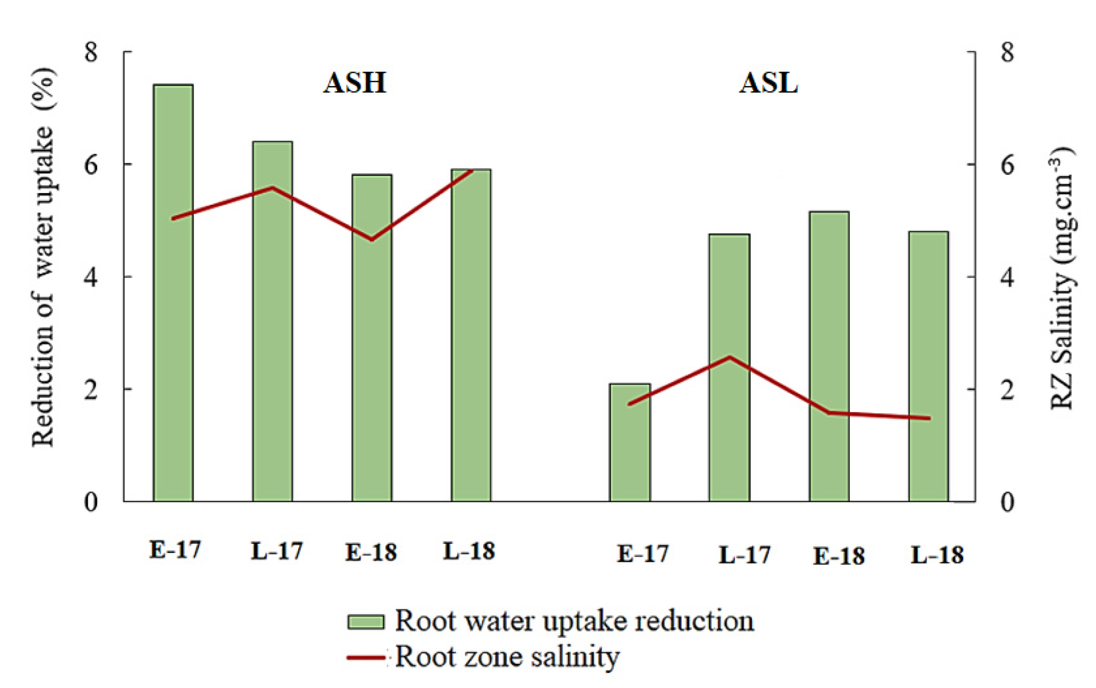
3.3. Salinity Impacts on Root Water Uptake

The reduction in water uptake by trees (Tr reduction) due to the salinity stress was estimated as follows:
T r   reduction = 1 Actual   root   water   uptake / season Potential   root   water   uptake / season
The reductions in HYDRUS-1D-simulated actual transpiration fluxes (i.e., root water uptake) were related to root zone salinities in Figure 12 for different parts of the growing season. In SJV, CA, the almond growing season starts after a winter dormancy in January and ends in August. The growing season of pistachios begins in late March and ends in September (Table 3). We analyzed the effects of simulated root zone salinities on the water uptake reduction in west and east SJV by comparing the ASH and ASL sites, respectively. The comparison was carried out for two periods, the early time of the growing season (“E”) and the late time of the growing season (“L”). The analysis includes the wet year 2017, followed by the dry year 2018. The seasonal deficit in crop growth is assumed to be related to the reduction in root water uptake (tree transpiration) due to salinity stress.
Average rootzone soil salinities in the early and late seasons in both east (ASL) and west (ASH) SJV during years 2017 and 2018 are shown in Figure 12. The early growing season (“E”) is February–March, when soil salinity reflects the impact of winter rains. On the other hand, the late growing season (“L”) is July–August, when soil salinity reflects the impact of irrigation water quality. Initial soil salinity at the ASH site in west SJV is relatively high compared to that at the ASL site in east SJV. As shown by E-17 (early season 2017) for the ASH site, the initially high salinity causes a relatively high reduction in root water uptake (almost 8%). Initial root zone soil salinity measured at the ASL site is lower than at the ASH site. Accordingly, at the ASL site, the reduction in root water uptake was low in the wet year (E-17) and increased in the dry year (E-18). The rain had a higher impact on reducing soil salinity when initial soil salinity was lower, and irrigation with less saline water was used. Root zone salinity decreased by 15% at the ASL site (during E-17 and E-18). The correlation between the root water uptake reduction and the root zone salinity is highly significant (the P one-tail value is 0.03). At the high salinity ASH site, the soil salinity increased by 10% and 26% in wet and dry years, respectively, while water uptake was reduced during both E-17 to E-18 by 20%.
The late growing season (“L”) is when soil salinity reflects the impact of irrigation. The effect of irrigation was higher at the ASH site (with initial high salinity) than at the ASL site (with initial low salinity). At the ASH site, root zone soil water salinity in the late season increased during both wet and dry years (i.e., L-17 and L-18, respectively). At the ASL site, root zone salinity increased only in the wet year (L-17) but decreased in the dry year (L-18). The degree of root zone salinity increase or decrease did not significantly affect root water uptake reduction in both years at the ASL site (with initial low salinity). We attribute the reduction in root zone salinity during L-18 at the ASL site to the leaching practice, which successfully maintained root water uptake during both dry (i.e., L-18) and wet (i.e., L-17) years.
The ASH and ASL sites are commercial orchards where current root zone salinities are mostly below the almond and pistachio salinity threshold values (discussed in Section 2.2). The maximum reduction in potential water uptake (7%) occurred at the (initially saline) ASH site. This simulated high reduction in root water uptake reflects the effects of continued irrigations with highly saline water in the west SJV. The reduction in root water uptake at the ASL site in response to both low initial soil salinity conditions and the wet year (ASL, E-17) was the lowest (2.5%). In conclusion, the minimum reduction in root water uptake occurred during the wet year 2017 at the site with low root zone salinity at the beginning of the growing season.

3.4. The Impact of Salt Leaching on Root Water Uptake

The leaching fraction indicates the degree to which salts are leached from the root zone [56]. Micro-irrigation’s leaching efficiency can be expressed as a ratio of the salt reduction to the equivalent leaching depth [57]. The leaching fraction is defined as a fraction of applied irrigation and rain that drains beyond the root zone [58]. Fractions of water leached below the root zone were estimated from the simulated top and bottom cumulative water fluxes. Leaching fractions showed a similar increase spike at all sites during winter (December 2016 and December 2017), when the uptake reductions decreased at all sites accordingly.
Table 6 provides information about correlations between a reduction in root water uptake and leaching fractions. Most values in the table above showed a significant negative correlation between leaching fractions (which positively affect reducing root zone salinity) and water uptake reduction. Negative correlations (Table 6) indicate that the lower the leaching fraction, the higher the water uptake reduction. For example, at the ASH site in the west SJV, a significant negative correlation (−0.91) between the leaching fraction and root water uptake reduction was achieved, which means that decreased leaching in early 2017 was correlated with an increase in root water uptake reduction. In addition, at the ASL site in the eastern SJV, the root water uptake reduction was always negatively associated with the leaching fraction (−0.95, −0.93, and −0.45) except for the early time of the wet year 2017.
When leaching fractions showed a low positive correlation with a root water uptake reduction (i.e., 0.23 at the ASH site and 0.41 at the ASL site, Table 6), then an increase in leaching was positively correlated with an increase in water uptake reductions. This increase in the water uptake reduction is more closely correlated with the effects of the saline irrigation water use in prior years than with the rain year type (and thus leaching) during the measurement time.

4. Summary and Conclusions

The HYDRUS-1D model was used to evaluate experimental data collected at four sites in SJV, California (ASH, ASL, ASM, PSH, and PSL), involving almond (A) and pistachio (P) orchards with high (SH) and low (SL) soil salinities. Calibration and validation of the HYDRUS-1D model were conducted using measured soil water contents and electrical conductivities. Water flow, soil water contents, root zone water leaching, and root water uptake were simulated at all five sites ASH, ASL, ASM, PSH, and PSL. However, only the ASH and ASL sites were successfully analyzed in terms of root zone water contents and root water uptake. At the other three sites, agreements between measured and simulated water contents were, for reasons discussed in Section 3.1, less suitable. Consequently, soil salinity at different root zone depths and salt leaching were simulated only for the ASL and ASH sites. The ASL and ASH sites were used to compare the effects of different irrigation waters, initial soil water salinities, and regional mean rainfalls between east and west SJV, CA.
Simulated actual evapotranspiration (ET) showed a suitable agreement with on-site eddy covariance measurements of actual ET at the ASL and ASH sites. The minimum root water uptake reduction was obtained during the wet year 2017 at the site with low root zone salinity at the beginning of the growing season (i.e., at the ASL site). The simulated water uptake reduction was highly negatively correlated with the leaching fraction. The more water drained (and salts leached), the less root water uptake was reduced.
The effect of rain on soil salinity at the ASL and ASH sites was evaluated for the early growing season when rain was a dominant factor for soil salinity and for the late growing season when irrigation water salinity was the dominant factor. Simulated higher leaching fractions showed higher root water uptake reductions in late seasons than in early seasons (Figure 12). During the early season, the root water uptake reduction at the ASH site was mainly caused by salinity accumulated during prior seasons and not adequately leached by winter rainfalls. Lowering salinity at the beginning of the growing season (either by winter rains or additional irrigation) is crucial for minimizing the risk of substantial crop water uptake reductions due to the potentially high salinity of irrigation water.
The suitable correspondence between simulated and measured root zone salinities and SWCs obtained in this study for the ASL and ASH sites will enable us in a further study to use HYDRUS-1D to predict future root zone salinity trends at these sites for various future climate scenarios. The base simulations and the calibrated model presented in this manuscript will allow us to evaluate the impacts of likely future climate change scenarios on the sustainability of almond orchards agriculture in SJV and to provide management recommendations considering available water resources and their quality to mitigate any negative and adverse impacts of anticipated future climate change. We will not be able to do that for the other three sites, for which the agreements between measured and simulated water contents were, for various reasons, less suitable than at the ASL and ASH sites.

Author Contributions

Conceptualization, methodology, resources, supervision, project administration, funding acquisition: T.H.S., R.G.A. and J.Š.; software: J.Š. and S.A.H.; formal analysis: S.A.H.; investigation: S.A.H., J.Š., T.H.S. and R.G.A.; data curation: T.H.S.; writing—original draft preparation: S.A.H.; writing—review and editing: J.Š., T.H.S. and R.G.A.; visualization: S.A.H. All authors have read and agreed to the published version of the manuscript.

Funding

This work was funded by the USDA-ARS Office of National Programs (project 2036-61000-018-00-D) and USDA (CA-R-ENS-5047-RR and CA-R-ENS-7274-H).

Institutional Review Board Statement

Not applicable.

Informed Consent Statement

Not applicable.

Data Availability Statement

Eddy covariance data are available via Ameriflux. Other data are available upon reasonable request to the corresponding authors.

Acknowledgments

The authors would like to thank Dennise Jenkins, Towfiq Khan, and Kailuh Menefee for their assistance with field and laboratory work.

Conflicts of Interest

The authors declare no conflict of interest.

References

  1. Green, T.R.; Ahuja, L.R.; Benjamin, J.G. Advances and Challenges in Predicting Agricultural Management Effects on Soil Hydraulic Properties. Geoderma 2003, 116, 3–27. [Google Scholar] [CrossRef]
  2. Schoups, G.; Hopmans, J.W.; Young, C.A.; Vrugt, J.A.; Wallender, W.W.; Tanji, K.K.; Panday, S. Sustainability of Irrigated Agriculture in the San Joaquin Valley, California. Proc. Natl. Acad. Sci. USA 2005, 102, 15352–15356. [Google Scholar] [CrossRef] [Green Version]
  3. Li, X.; Kang, Y.; Wan, S.; Chen, X.; Liu, S.; Xu, J. Response of a Salt-Sensitive Plant to Processes of Soil Reclamation in Two Saline-Sodic, Coastal Soils Using Drip Irrigation with Saline Water. Agric. Water Manag. 2016, 164, 223–234. [Google Scholar] [CrossRef]
  4. Li, H.; Yi, J.; Zhang, J.; Zhao, Y.; Si, B.; Hill, R.L.; Cui, L.; Liu, X. Modeling of Soil Water and Salt Dynamics and Its Effects on Root Water Uptake in Heihe Arid Wetland, Gansu, China. Water 2015, 7, 2382–2401. [Google Scholar] [CrossRef] [Green Version]
  5. Phogat, V.; Pitt, T.; Cox, J.W.; Šimůnek, J.; Skewes, M.A. Soil Water and Salinity Dynamics under Sprinkler Irrigated Almond Exposed to a Varied Salinity Stress at Different Growth Stages. Agric. Water Manag. 2018, 201, 70–82. [Google Scholar] [CrossRef] [Green Version]
  6. Phogat, V.; Mallants, D.; Cox, J.W.; Šimůnek, J.; Oliver, D.P.; Awad, J. Management of Soil Salinity Associated with Irrigation of Protected Crops. Agric. Water Manag. 2020, 227. [Google Scholar] [CrossRef]
  7. Ramos, T.B.; Darouich, H.; Šimůnek, J.; Gonçalves, M.C.; Martins, J.C. Soil Salinization in Very High-Density Olive Orchards Grown in Southern Portugal: Current Risks and Possible Trends. Agric. Water Manag. 2019, 217. [Google Scholar] [CrossRef] [Green Version]
  8. Suarez, D.L. Modeling transient root zone salinity (SWS model). In Agricultural Salinity Assessment and Management; Wallender, W.W., Tanji, K.K., Eds.; American Society of Civil Engineers: Reston, VA, USA, 2011; pp. 856–897. ISBN 978-0-7844-1169-8. [Google Scholar]
  9. Minhas, P.S.; Ramos, T.B.; Ben-Gal, A.; Pereira, L.S. Coping with Salinity in Irrigated Agriculture: Crop Evapotranspiration and Water Management Issues. Agric. Water Manag. 2020, 227, 105832. [Google Scholar] [CrossRef]
  10. Shrivastava, P.; Kumar, R. Soil Salinity: A Serious Environmental Issue and Plant Growth Promoting Bacteria as One of the Tools for Its Alleviation. Saudi J. Biol. Sci. 2015, 22, 123–131. [Google Scholar] [CrossRef] [Green Version]
  11. Lobell, D.B.; Burke, M.B. On the Use of Statistical Models to Predict Crop Yield Responses to Climate Change. Agric. For. Meteorol. 2010, 150, 1443–1452. [Google Scholar] [CrossRef]
  12. Rasouli, F.; Kiani Pouya, A.; Šimůnek, J. Modeling the Effects of Saline Water Use in Wheat-Cultivated Lands Using the UNSATCHEM Model. Irrig. Sci. 2013, 31, 1009–1024. [Google Scholar] [CrossRef] [Green Version]
  13. Kumar, R.; Shankar, V.; Jat, M.K. Evaluation of Root Water Uptake Models—A Review. ISH J. Hydraul. Eng. 2015, 21, 115–124. [Google Scholar] [CrossRef]
  14. Šimůnek, J.; Šejna, M.; Saito, H.; Sakai, M.; Van Genuchten, M. The HYDRUS-1D Software Package for Simulating the One-Dimensional Movement of Water, Heat, and Multiple Solutes in Variably-Saturated Media; Version 4.17, HYDRUS Software Series 3; Department of Environmental Sciences, University of California Riverside: Riverside, CA, USA, 2008. [Google Scholar]
  15. Feddes, R.A.; Raats, P.A.C. Parameterizing the soil–water–plant root system. In Unsaturated-Zone Modeling; Progress, Challenges and Applications; Feddes, R.A., de Rooij, G.H., van Dam, J.C., Eds.; Wageningen UR Frontis Series; Kluwer Academic Publishers: Dordrecht, The Netherlands, 2004; pp. 95–141. ISBN 978-1-4020-2918-9. [Google Scholar]
  16. Oster, J.D.; Letey, J.; Vaughan, P.; Wu, L.; Qadir, M. Comparison of Transient State Models That Include Salinity and Matric Stress Effects on Plant Yield. Agric. Water Manag. 2012, 103, 167–175. [Google Scholar] [CrossRef]
  17. Gigante, V.; Iacobellis, V.; Manfreda, S.; Milella, P.; Portoghese, I. Influences of Leaf Area Index Estimations on Water Balance Modeling in a Mediterranean Semi-Arid Basin. Nat. Hazards Earth Syst. Sci. 2009, 9, 979–991. [Google Scholar] [CrossRef] [Green Version]
  18. Letey, J.; Hoffman, G.J.; Hopmans, J.W.; Grattan, S.R.; Suarez, D.; Corwin, D.L.; Oster, J.D.; Wu, L.; Amrhein, C. Evaluation of Soil Salinity Leaching Requirement Guidelines. Agric. Water Manag. 2011, 98, 502–506. [Google Scholar] [CrossRef] [Green Version]
  19. Kaledhonkar, M.J.; Keshari, A.K. Modelling the Effects of Saline Water Use in Agriculture. Irrig. Drain. 2006, 55, 177–190. [Google Scholar] [CrossRef]
  20. Kaledhonkar, M.J.; Sharma, D.R.; Tyagi, N.K.; Kumar, A.; Van Der Zee, S.E.A.T.M. Modeling for Conjunctive Use Irrigation Planning in Sodic Groundwater Areas. Agric. Water Manag. 2012, 107, 14–22. [Google Scholar] [CrossRef]
  21. Gonçalves, M.C.; Šimůnek, J.; Ramos, T.B.; Martins, J.C.; Neves, M.J.; Pires, F.P. Multicomponent Solute Transport in Soil Lysimeters Irrigated with Waters of Different Quality. Water Resour. Res. 2006, 42. [Google Scholar] [CrossRef] [Green Version]
  22. Ramos, T.B.; Šimůnek, J.; Gonçalves, M.C.; Martins, J.C.; Prazeres, A.; Castanheira, N.L.; Pereira, L.S. Field Evaluation of a Multicomponent Solute Transport Model in Soils Irrigated with Saline Waters. J. Hydrol. 2011, 407, 129–144. [Google Scholar] [CrossRef]
  23. Zeng, Z.; Wang, T.; Zhou, F.; Ciais, P.; Mao, J.; Shi, X.; Piao, S. A Worldwide Analysis of Spatiotemporal Changes in Water Balance-Based Evapotranspiration from 1982 to 2009. J. Geophys. Res. Atmos. 2014, 119, 1186–1202. [Google Scholar] [CrossRef]
  24. Suarez, D.L.; Wood, J.D.; Lesch, S.M. Effect of SAR on Water Infiltration under a Sequential Rain–Irrigation Management System. Agric. Water Manag. 2006, 86, 150–164. [Google Scholar] [CrossRef]
  25. Haj-Amor, Z.; Ibrahimi, M.-K.; Feki, N.; Lhomme, J.-P.; Bouri, S. Soil Salinisation and Irrigation Management of Date Palms in a Saharan Environment. Environ. Monit. Assess. 2016, 188, 497. [Google Scholar] [CrossRef] [PubMed]
  26. Ramos, T.B.; Šimůnek, J.; Gonçalves, M.C.; Martins, J.C.; Prazeres, A.; Pereira, L.S. Two-Dimensional Modeling of Water and Nitrogen Fate from Sweet Sorghum Irrigated with Fresh and Blended Saline Waters. Agric. Water Manag. 2012, 111, 87–104. [Google Scholar] [CrossRef]
  27. Wang, J.; Bai, Z.; Yang, P. Mechanism and Numerical Simulation of Multicomponent Solute Transport in Sodic Soils Reclaimed by Calcium Sulfate. Environ. Earth Sci. 2014, 72, 157–169. [Google Scholar] [CrossRef]
  28. Schaap, M.G.; Leij, F.J.; van Genuchten, M.T. Rosetta: A Computer Program for Estimating Soil Hydraulic Parameters with Hierarchical Pedotransfer Functions. J. Hydrol. 2001, 251, 163–176. [Google Scholar] [CrossRef]
  29. van Genuchten, M.T. A Closed-Form Equation for Predicting the Hydraulic Conductivity of Unsaturated Soils. Soil Sci. Soc. Am. J. 1980, 44, 892–898. [Google Scholar] [CrossRef] [Green Version]
  30. Jacques, D.; Šimůnek, J.; Timmerman, A.; Feyen, J. Calibration of Richards’ and Convection–Dispersion Equations to Field-Scale Water Flow and Solute Transport under Rainfall Conditions. J. Hydrol. 2002, 259, 15–31. [Google Scholar] [CrossRef]
  31. Helalia, S.A.; Anderson, R.G.; Skaggs, T.H.; Jenerette, G.D.; Wang, D.; Šimůnek, J. Impact of Drought and Changing Water Sources on Water Use and Soil Salinity of Almond and Pistachio Orchards: 1. Observations. Soil Syst. 2021, 5, 50. [Google Scholar] [CrossRef]
  32. Anderson, R. AmeriFlux US-ASH USSL San Joaquin Valley Almond High Salinity. 2020. Available online: https://ameriflux.lbl.gov/sites/siteinfo/US-ASH (accessed on 1 September 2020).
  33. Anderson, R. AmeriFlux US-ASM USSL San Joaquin Valley Almond Medium Salinity. 2020. Available online: https://ameriflux.lbl.gov/sites/siteinfo/US-ASM (accessed on 1 September 2020).
  34. Anderson, R. AmeriFlux US-ASL USSL San Joaquin Valley Almond Low Salinity. 2020. Available online: https://ameriflux.lbl.gov/sites/siteinfo/US-ASL (accessed on 1 September 2020).
  35. Anderson, R. AmeriFlux US-PSH USSL San Joaquin Valley Pistachio High. 2020. Available online: https://ameriflux.lbl.gov/sites/siteinfo/US-PSH (accessed on 1 September 2020).
  36. Anderson, R. AmeriFlux US-PSL USSL San Joaquin Valley Pistachio Low. 2020. Available online: https://ameriflux.lbl.gov/sites/siteinfo/US-PSL (accessed on 1 September 2020).
  37. Holm, L.; Podger, D.; Harader, S.; Fernandez, P.; Ullrey, R.; Li, X.; McCarthy, M.; Larsen, K.; Burau, J.; Orloff, L.; et al. Conceptual Model For Salinity in the Central Valley and Sacramento-San Joaquin Delta; CALFED Bay-Delta Program: Sacramento, CA, USA, 2007; p. 65. [Google Scholar]
  38. Almond Board of California. Almond Almanc; Almond Board of California: Modesto, CA, USA, 2018; p. 25. [Google Scholar]
  39. Šimůnek, J.; van Genuchten, M.T.; Šejna, M. Recent Developments and Applications of the HYDRUS Computer Software Packages. Vadose Zone J. 2016, 15. [Google Scholar] [CrossRef] [Green Version]
  40. Richards, L.A. Capillary conduction of liquids through porous mediums. Physics 1931, 1, 318–333. [Google Scholar] [CrossRef]
  41. Allen, R.G.; Pereira, L.S.; Raes, D.; Smith, M. Crop Evapotranspiration: Guidelines for Computing Crop Water Requirements; Food and Agriculture Organization of the United Nations: Rome, Italy, 1998; ISBN 92-5-104219-5. [Google Scholar]
  42. Zheng, C.; Lu, Y.; Guo, X.; Li, H.; Sai, J.; Liu, X. Application of HYDRUS-1D Model for Research on Irrigation Infiltration Characteristics in Arid Oasis of Northwest China. Environ. Earth Sci. 2017, 76, 785. [Google Scholar] [CrossRef]
  43. Raz-Yaseef, N.; Yakir, D.; Schiller, G.; Cohen, S. Dynamics of Evapotranspiration Partitioning in a Semi-Arid Forest as Affected by Temporal Rainfall Patterns. Agric. For. Meteorol. 2012, 157, 77–85. [Google Scholar] [CrossRef]
  44. Melton, F.S.; Johnson, L.F.; Lund, C.P.; Pierce, L.L.; Michaelis, A.R.; Hiatt, S.H.; Guzman, A.; Adhikari, D.D.; Purdy, A.J.; Rosevelt, C.; et al. Satellite Irrigation Management Support With the Terrestrial Observation and Prediction System: A Framework for Integration of Satellite and Surface Observations to Support Improvements in Agricultural Water Resource Management. IEEE J. Sel. Top. Appl. Earth Obs. Remote Sens. 2012, 5, 1709–1721. [Google Scholar] [CrossRef]
  45. van Genuchten, M.T.; Hoffman, G.J.; Hanks, R.J.; Meiri, A.; Shalhevet, J.; Kafkafi, U. Management Aspect for Crop Production. In Soil Salinity under Irrigation; Shainberg, I., Shalhevet, J., Eds.; Springer Berlin Heidelberg: Berlin/Heidelberg, Germany, 1984; pp. 258–338. ISBN 978-3-642-69836-1. [Google Scholar]
  46. Skaggs, T.H.; van Genuchten, M.T.; Shouse, P.J.; Poss, J.A. Macroscopic Approaches to Root Water Uptake as a Function of Water and Salinity Stress. Agric. Water Manag. 2006, 86, 140–149. [Google Scholar] [CrossRef]
  47. Grismer, M.E. Leaching Fraction, Soil Salinity, and Drainage Efficiency. Calif. Agric. 1990, 44, 24–26. [Google Scholar] [CrossRef]
  48. Maas, E.V.; Hoffman, G. Crop Salt Tolerance—Current Assessment. J. Irrig. Drain. Div.-ASCE 1977, 103, 115–134. [Google Scholar] [CrossRef]
  49. Maas, E.V. Crop salt tolerance. In Agricultural Salinity Assessment and Management; Tanji, K.K., Ed.; ASCE manuals and reports on engineering practice; American Society of Civil Engineers: New York, NY, USA, 1990; pp. 262–304. ISBN 978-0-87262-762-8. [Google Scholar]
  50. Sanden, B.L.; Ferguson, L.; Reyes, H.C.; Grattan, S.R. Effect of salinity on evapotranspiration and yield of San Joaquin Valley pistachios. In Proceedings of the Acta Horticulturae; International Society for Horticultural Science (ISHS): Leuven, Belgium, 2004; pp. 583–589. [Google Scholar]
  51. Sepaskhah, A.R.; Maftoun, M. Relative Salt Tolerance of Pistachio Cultivars. J. Hortic. Sci. 1988, 63, 157–162. [Google Scholar] [CrossRef]
  52. Hanson, B.R.; Šimůnek, J.; Hopmans, J.W. Evaluation of Urea–Ammonium–Nitrate Fertigation with Drip Irrigation Using Numerical Modeling. Agric. Water Manag. 2006, 86, 102–113. [Google Scholar] [CrossRef]
  53. Gärdenäs, A.I.; Hopmans, J.W.; Hanson, B.R.; Šimůnek, J. Two-Dimensional Modeling of Nitrate Leaching for Various Fertigation Scenarios under Micro-Irrigation. Agric. Water Manag. 2005, 74, 219–242. [Google Scholar] [CrossRef]
  54. Weihermüller, L.; Kasteel, R.; Vanderborght, J.; Pütz, T.; Vereecken, H. Soil Water Extraction with a Suction Cup: Results of Numerical Simulations. Vadose Zone J. 2005, 4, 899–907. [Google Scholar] [CrossRef]
  55. METER Group. GS3 Manual; METER Group: Pullman, DC, USA, 2019. [Google Scholar]
  56. US Salinity Laboratory. Diagnosis and Improvement of Saline and Alkali Soils; Richards, L.A., Ed.; Handbook; Soil and Water Conservative Research Branch, Agricultural Research Service, U.S. Dept. of Agriculture: Washington, DC, USA, 1954.
  57. Burt, C.M.; Isbell, B. Leaching of Accumulated Soil Salinity under Drip Irrigation. Trans. ASAE 2005, 48, 2115–2121. [Google Scholar] [CrossRef]
  58. Corwin, D.L.; Grattan, S.R. Are Existing Irrigation Salinity Leaching Requirement Guidelines Overly Conservative or Obsolete? J. Irrig. Drain. Eng. 2018, 144, 02518001. [Google Scholar] [CrossRef] [Green Version]
Figure 1. Measured relative spatial distributions (the maximum is one) of root densities of almond trees (top) at the ASL (left) and ASH (right) sites and of pistachio trees (bottom) at the PSL (left) and PSH (right) sites. The terms “Tower” and “Outlying” refer to sampling locations with respect to the eddy covariance tower [31].
Soilsystems 05 00058 g001
Figure 2. Effects of irrigation and rain on the measured and HYDRUS-1D simulated soil water contents at a depth of 25 cm at the ASL site (a) and the ASH site (b).
Soilsystems 05 00058 g002
Figure 3. Measured (dots) and simulated (lines) soil water contents at four root zone depths of 25, 50, 75, and 100 cm at the ASL site.
Soilsystems 05 00058 g003
Figure 4. Measured (dots) and simulated (lines) soil water contents at four root zone depths of 25, 50, 75, and 100 cm at the ASH site.
Soilsystems 05 00058 g004
Figure 5. Effects of irrigation and rain on the measured and HYDRUS-1D simulated soil water contents at a depth of 25 cm at the ASM site.
Soilsystems 05 00058 g005
Figure 6. Effects of irrigation and rain on the measured and HYDRUS-1D simulated soil water contents at a depth of 25 cm at the PSL site.
Soilsystems 05 00058 g006
Figure 7. Effects of irrigation and rain on the measured and HYDRUS-1D simulated soil water contents at a depth of 25 cm at the PSH site.
Soilsystems 05 00058 g007
Figure 8. Measured (dots) and simulated (lines) salinities at four observation depths of 25, 50, 75, and 100 cm at the ASL site.
Soilsystems 05 00058 g008
Figure 9. Measured (dots) and simulated (lines) electrical conductivities at four observation depths of 25, 50, 75, and 100 cm at the ASH site.
Soilsystems 05 00058 g009
Figure 10. Seasonal (fall, winter, spring, and summer) simulated and measured root zone salinities at the low and high saline ASL and ASH sites, respectively, during the wet year 2017 (a) and the dry year 2018 (b).
Soilsystems 05 00058 g010
Figure 11. Simulated and measured actual evapotranspiration at (a) the ASL site and (b) the ASH site.
Soilsystems 05 00058 g011
Figure 12. Simulated root zone salinities and corresponding reductions in tree water uptake at the ASH site (west SJV) and the ASL site (east SJV). “E” refers to the early growing season (February–March period), and “L” refers to the late growing season (July–August period).
Soilsystems 05 00058 g012
Table 1. List of study orchards and their characteristics.
Site NameAmeri Flux DesignationSoil TypeMean Annual Rain (mm)Initial Salinity (dS/m)Initial SAR
(mmol/L)0.5
Almond Salinity HighUS-ASHClay Loam<2002.2–4.17–25
Almond Salinity MediumUS-ASMSilty Clay Loam<2001.8–3.57–20
Pistachio Salinity HighUS-PSHSilty Clay<2002.3–4.75–15
Almond Salinity LowUS-ASLSandy Loam>2501.3–1.910–25
Pistachio Salinity LowUS-PSLSandy Loam>2501.1–2.13–10
Table 2. Irrigation water salinity, sodicity, and ionic composition at four experimental sites.
SitesDay of Water CollectionECiw (dS·m−1)SARpHCa2+Mg2+Na+K+
(mmolc/L)0.5(mmolc·L−1)
PSL30 March 20170.050.487.640.10.020.190.05
30 March 20170.040.67.60.080.010.130.04
5 July 20170.24 7.80.490.241.150.07
17 May 20180.04 7.20.080.020.190.04
2 August 20180.05 8.060.070.010.150.04
ASH30 May 20170.3 7.780.320.321.290.17
11 August 20170.241.47.140.350.351.540.09
6 July 20180.43 7.61.040.512.240.1
19 September 20180.54 6.950.310.291.090.07
20 January 20190.79 7.81.11.164.760.19
ASM30 May 20170.281.77.70.330.331.470.08
17 May 20180.43 7.690.870.582.470.13
6 July 20180.541.87.720.430.613.260.12
6 July 20180.531.881.111.24.920.24
19 September 20180.51 7.890.460.522.310.11
5 January 20180.48 7.80.910.695.980.14
PSH20 February 20180.44 7.570.520.592.860.16
31 August 20180.894.17.720.510.562.540.12
19 September 20180.4837.930.440.573.030.11
30 January 20190.9 7.771.220.745.890.09
Table 3. Growing seasons in the San Joaquin Valley for almond and pistachio.
CropGrowing SeasonEarly SeasonLate Season
AlmondFebruary–AugustFebruary–MarchJuly–August
PistachioApril–SeptemberApril–MayAugust–September
Table 4. The soil hydraulic parameters for four depths of five experimental sites.
SitesDepth
(cm)
θr
(cm3·cm−3)
θs
(cm3·cm−3)
α
(cm−1)
n
(-)
Ks
(cm·d−1)
ASL250.0390.3950.0201.4929.2
500.0410.4640.0201.5117.7
750.0470.4040.0141.4821.8
1000.0360.3490.0171.5327.8
ASH250.0720.3430.0091.3016.2
500.0980.4330.0021.715.6
750.1170.8470.0031.750.5
1000.1160.9350.0031.662.1
ASM250.0980.5030.0141.3919.8
500.0940.4860.0131.3118.3
750.0920.4900.0101.4820.6
1000.0920.4900.0101.4820.6
PSL250.0380.5230.0401.5551.0
500.0350.4230.0241.2630.4
750.0400.5500.0361.5030.3
1000.0350.3760.0411.5213.8
PSH250.1010.4800.0161.3321.9
500.1010.5030.0161.337.03
750.0990.4940.0151.357.03
1000.0930.4780.0131.4013.6
Table 5. RMSE (dimensionless) for simulated volumetric water content and measured.
ASH, West SJV, CAASL, East SJV, CA
0–25 cm25–50 cm50–75 cm75–100 cm0–25 cm25–50 cm50–75 cm75–100 cm
0.0540.150.280.250.0560.0590.0630.033
Table 6. Pearson correlation between a reduction in root water uptake and leaching fractions.
ASH, West SJV, CAASL, East SJV, CA
Wet 2017Dry 2018Wet 2017Dry 2018
EarlyLateEarlyLateEarlyLateEarlyLate
−0.912 **0.2360.2360.955 **0.419 **−0.949 **−0.933 **−0.436 **
** Correlation is significant at the 0.01 level (2-tailed).
Publisher’s Note: MDPI stays neutral with regard to jurisdictional claims in published maps and institutional affiliations.

