A New Method for Calculating the Hamaker Constant Based on the Hansen Solubility Parameters for Non-Polar Liquids

Abstract

A simple relationship between the Hamaker constant and the Hansen solubility parameters for non-polar liquids is derived by combining a Hamaker constant/surface tension relationship derived by Israelachvili and a Hansen solubility parameters/surface tension relationship derived by Abbott. With this relationship, one can easily estimate the Hamaker constant of non-polar liquids on the basis of the database of the Hansen solubility parameters. This is an entirely new method for calculating the Hamaker constant without recourse to data on the frequency-dependent dielectric permittivity of those substances (which are required for the rigorous Lifshitz theory) and laborious numerical calculations.

1. Introduction

When two molecules or atoms are approaching each other, attractive intermolecular or interatomic forces, which are called the van der Waals forces, are acting between these two molecules or atoms. There are three types of intermolecular van der Waal interactions: (i) the Keesom interaction due to permanent electric dipole–dipole interaction between two polar molecules; (ii) the Debye interaction, which is the permanent dipole-induced dipole interaction between polar and nonpolar molecules; and (iii) the dispersion interaction between quantum mechanically fluctuating dipoles induced within the interacting molecules. The van der Waals attractive interaction energy acting between two molecules separated by a distance r is proportional to 1/r⁶, as shown later in Equation (1), making it extremely short-ranged. Among these three van der Waals interactions, the contribution of the dispersion interaction is the largest for non-polar molecules. Unlike strong covalent interactions, however, the van der Waals dispersion interaction does not exhibit saturation, lacks directionality, and demonstrates additive behavior. Therefore, a significantly large van der Waals attractive interaction is expected to operate between two approaching colloidal particles, which are composed of a large number of molecules.

Hamaker [1] considered attractive interaction forces of the same nature as the van der Waals intermolecular dispersion forces to act between two approaching colloidal particles composed of a large number of molecules. Hamaker calculated the van der Waals dispersion interaction energy between two colloidal particles by summing up the van der Waals dispersion interaction energies between molecules in one particle and those in another particle on the basis of the assumption that the intermolecular van der Waals dispersion interaction energy is additive.

The interparticle van der Waals dispersion interaction energy is found to be proportional to the Hamaker constant A and to 1/h² for the case of two parallel plates separated by a distance h, which is now a long-range attractive interaction [1], as is seen later in Equation (3). It is further seen from Equation (4) that the Hamaker constant A is proportional to the London–van der Waals constant C characterizing the intermolecular van der Waals dispersion interaction and the square of the number density N of the molecules within the interacting particles. Lifshitz [2] later developed a rigorous continuum theory of the van der Waals interaction between colloidal particles without recourse to the additivity approach of Hamaker and derived the exact expression for the Hamaker constant, expressed later in Equation (5). Note that while the Hamaker theory [1] accounts only for the van der Waals dissipative interactions, the Lifshitz theory [2] takes into account all of the above-mentioned three types of the van der Waals interactions as well as hydrogen-bond interactions.

The theoretical estimation of the Hamaker constant of substances based on Lifshitz’s rigorous theory, however, requires data on the frequency-dependent dielectric permittivity of those substances and involves laborious numerical calculations [2,3,4].

According to the Derjaguin–Landau–Verwey–Overbeek (DLVO) theory for the stability of colloidal suspensions [5,6], the Hamaker constant A plays a crucial role in determining the stability of colloidal suspensions [3,5,6,7,8]. That is, the van der Waals force acting between colloidal particles is an attractive force in colloidal dispersion systems and is characterized by the Hamaker constant A, serving as an aggregation enhancement factor that promotes the aggregation of dispersed systems. The magnitude of the Hamaker constant, which has the dimension of energy, typically falls within the range of 10⁻²⁰–10⁻¹⁹ J for non-polar liquids, corresponding to 10–100 times the thermal energy kT, where k is the Boltzmann constant and T is the absolute temperature. Further, it is important to note that the Hamaker constant of a substance is related to its cohesion energy and surface tension [3].

The Hamaker constant is practically important, particularly in the field of drug delivery systems (DDS). The Hamaker constant A, quantifying the van der Waals forces at the nanoscale, plays a crucial role in formulating and optimizing nanocarriers for drug delivery. Understanding the Hamaker constants aids researchers in designing nanosized drug carriers with enhanced stability, controlled release, and improved bioavailability. The intermolecular dispersion forces, influenced by the Hamaker constant A, impact the interaction between drug-loaded nanoparticles and biological interfaces, ultimately affecting the efficiency of drug delivery.

The history of Hansen solubility parameters, on the other hand, dates back to 1967 when Charles Hansen introduced this concept [9,10]. Hansen proposed a method to determine the solubility of substances with the help of the Hansen solubility parameter. Since the Hansen solubility parameter is widely adopted in fields such as chemistry, engineering, and materials science, it has become a valuable tool for substance design and product development, providing insights into compatibility for various applications.

The Hansen solubility parameter δ, which was introduced by Hansen [9,10], is a crucial parameter in the field of intermolecular interactions. The Hansen parameter provides a comprehensive framework for understanding the compatibility between different substances on the basis of their molecular interactions (see, e.g., [11]). That is, this parameter quantifies the cohesive energy density of a substance, representing the contributions from the dispersion forces δ_D, polar forces δ_P, and hydrogen bonding forces δ_H. These forces determine whether a substance will dissolve or mix well with another substance. The data for the Hansen solubility parameters for a large number of substances have so far been accumulated, and their extensive databases are now available for practical use [9,10].

The Hansen parameter is also important in the field of DDS. The Hansen parameters, characterizing the solubility and compatibility of materials, play a vital role in tailoring the formulations of drug carriers and biomaterials. By accounting for the dispersion, polar, and hydrogen bonding forces, one can precisely choose materials that enhance drug solubility, bioavailability, and targeted delivery. The Hansen parameters guide the selection and combination of polymers, coatings, and encapsulants, ensuring optimal compatibility with therapeutic agents. This understanding facilitates the development of DDS platforms that exhibit improved drug stability and controlled release profiles. The Hansen solubility parameter is thus a measure indicating the interaction between organic solvents and solutes based on molecular polarity and intermolecular forces. Comprising dispersion forces, dipole–dipole interactions, and hydrogen bonding, it helps understand how substances interact. This parameter facilitates the prediction of interactions between specific solvents and materials, contributing to material design and optimizing chemical processes.

The Hansen parameter has been increasingly recognized not only in the field of solution chemistry but also in the field of colloid and interface science. For example, the Hansen parameters are highly useful when selecting the most suitable dispersant for dispersing colloidal systems. Fairhurst et al. [12] demonstrated the crucial importance of choosing the right solvent to disperse sub-micron particles for optimal product performance. Utilizing solvent relaxation NMR, they effectively evaluated the suitability of the solvent. This technique, responsive to intermolecular forces, functions as a dependable indicator of dispersion stability. Employing a systematic relaxation measurement approach, they obtained the Hansen solubility parameters for particle surfaces, facilitating precise solvent selection and blending to align with the particle interface. For the case of surface-modified zinc oxide and aluminum oxide particles, this approach clears subtle distinctions in particle surfaces. Saita et al. [13] reported that optimizing stabilizers and solvents is crucial for nanoparticle inks. They used the Hansen solubility parameters for oleylamine-capped silver nanoparticles and found that the Hansen solubility parameter approach quantitatively predicts the dispersibility of these nanoparticles, correlating with the sintered film morphology for electronic applications. This method contributes to the optimization of stabilizers and solvents for creating stable nanoparticle inks in the field of printed electronics.

As mentioned earlier, the Hamaker constant can be estimated with the help of the rigorous Lifshitz theory [2,3,4] but it requires tedious numerical calculations. The purpose of the present paper is to derive a simple relationship between the Hamaker constant A and the Hansen solubility parameters δ (δ_D, δ_P, and δ_H) for non-polar liquids. By using the obtained A/δ relationship, one can easily estimate the value of the Hamaker constant A of non-polar liquids based on the rigorous Lifshitz theory without recourse to data on the frequency-dependent dielectric permittivity of the liquid and laborious numerical calculations. This will be an entirely new method for estimating the Hamaker constant of non-polar liquids.

2. The Relationship between the Hamaker Constant and the Hansen Solubility Parameters

2.1. Hamaker Constant and Surface Tension

The potential energy u(r) of the van der Waals dispersion interaction between two similar molecules at a separation r between their centers in air, which can be regarded as a vacuum, is given by [1,3,7,8] as

$$u\left(r\right)=-\frac{C}{r^6}$$

(1)

with

$$C=\frac{3{\alpha }^{2}h\nu }{4{\left(4\pi {\epsilon }_0\right)}^2}$$

(2)

where C is the London–van der Waals constant, α and ν are, respectively, the electronic polarizability and the characteristic frequency of the molecule, ε₀ is the permittivity of a vacuum, h is the Planck constant, and hν corresponds to the ionization energy of the molecule.

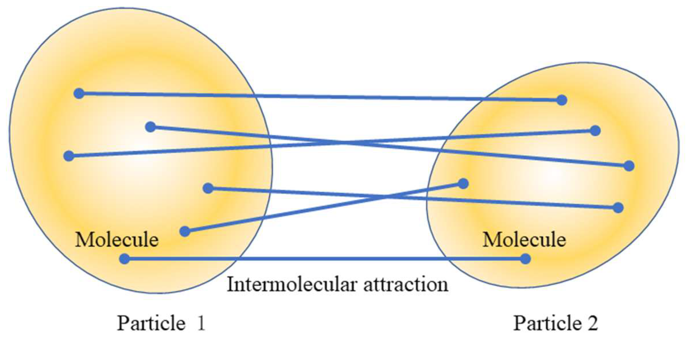
Hamaker [1] noticed that since the additivity of the van der Waals dispersion interactions holds quite well, the van der Waals dispersion interaction energy between two particles in a vacuum may thus be calculated approximately by a summation (or by an integration) of the dispersion interaction energies for all molecular pairs formed by two molecules belonging to different particles, as shown in Figure 1.

Hamaker [1] calculated the van der Waals dispersion interaction energy V(h) per unit area between two parallel plates at separation h between their surfaces across a vacuum by summing up the intermolecular interaction energy u(r) given in Equation (1), with the result that

$$V\left(h\right)=-\frac{A}{12\pi h^2}$$

(3)

In Equation (3), the parameter A is the Hamaker constant defined by

$$A={\pi }^{2}C{N}^2$$

(4)

where C is the London–van der Waals constant given in Equation (2).

Hamaker’s classical theory [1] of the van der Waals attractive interaction accounts only for the additive London dispersion interaction between molecules but ignores the two other intermolecular van der Waals interactions, that is, the Keesom interaction between two permanent electric dipoles and the Debye interaction between permanent and induced electric dipoles, unlike the theory by Hansen [9], which considers not only the dispersion interaction but also polar interactions and hydrogen-bonding interactions. Lifshitz [2] later presented a modern continuum theory of the van der Waals interaction energy, showing that the interaction energy between two parallel plates takes the same dependence on the plate separation h (Equation (3)) if the retardation effect may be neglected. Lifshitz derived the following rigorous expression for the Hamaker constant A for the van der Waals attractive interaction between two identical particles on the basis of the continuum approach:

$$A=\frac{3h}{16{\pi }^2}{\int }_0^{\infty }d\omega {\int }_0^{\infty }\frac{x^2}{\left[\frac{{\left\{{\epsilon }_{\mathrm{r}}\left(i\omega \right)+1\right\}}^2}{{\left\{{\epsilon }_{\mathrm{r}}\left(i\omega \right)-1\right\}}^2}{e}^x-1\right]}dx$$

(5)

where ε_r(iω) is the frequency ω-dependent relative permittivity of the particles, and i is the imaginary unit. The following approximate expression for the Hamaker constant has also been proposed [3]:

$$A=\frac{3h\nu }{16\sqrt{2}}\frac{{\left(n^2-1\right)}^2}{{\left(n^2+1\right)}^{3/2}}+\frac{3}{4}kT{\left(\frac{{\epsilon }_{\mathrm{r}}-1}{{\epsilon }_{\mathrm{r}}+1}\right)}^2$$

(6)

where n is the refraction index. In Equation (6), the first term on the right-hand side is the interaction at the main ultraviolet frequency ν corresponding to electronic absorption. It accounts for the London dispersion force, while the second term, which is proportional to the absolute temperature T, is the interaction at zero frequency and contains both the Debye and Keesom interactions.

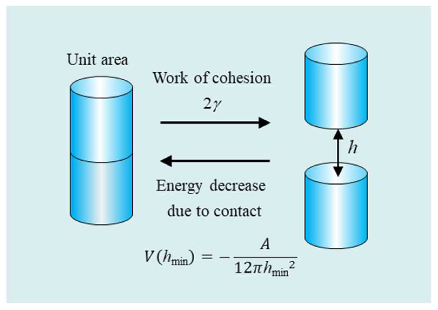
In order to find the relationship between the Hamaker constant A and the surface tension γ of a liquid, we consider two cylinders with two flat surfaces of unit area in contact with each other and those separated by a distance h (Figure 2). It follows from Equation (3) that the energy required to bring the two cylinders from infinity into contact (at h = h_min) is given by

$$V\left(h_{\mathrm{m}\mathrm{i}\mathrm{n}}\right)=-\frac{A}{12\pi h_{\mathrm{m}\mathrm{i}\mathrm{n}}^2}$$

(7)

where h_min is the closest separation distance between the surfaces of the two approaching cylinders and it has the same order of magnitude as the molecular diameter. Conversely, the energy required to separate these two cylinders from contact at h = h_min into infinity (h = ∞) is given by the negative of V(h_min) (Figure 2).

This energy V(h_min) is the cohesion (or cohesive) energy and is equal to the work to generate two unit surfaces of the substance, which amounts to 2γ, γ being the surface tension of the substance, so that we obtain

$$\gamma =\frac{A}{24\pi h_{\mathrm{m}\mathrm{i}\mathrm{n}}^2}$$

(8)

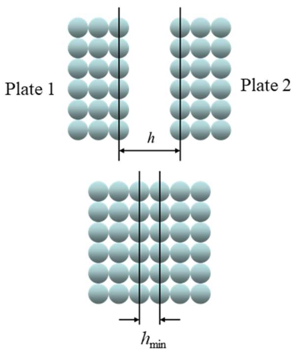
Note here that the closest distance between two flat surfaces may seem to be exactly the molecular diameter (Figure 3). Upon closer examination, however, due to the microscale surface structure caused by the arrangement of molecules, the closest distance between the two flat surfaces becomes smaller than the molecular diameter. Note also that the continuum theory by Lifshitz [2] can be applied only for distances much larger than the molecular dimension so that the determination of h_min, which should have the same order of magnitude as the molecular diameter, requires Hamaker’s molecular approach [1] as well as the continuum approach [3].

Israelachvili [3] rigorously derived the expression for h_min as follows: Let us obtain the value of h_min following Israelachvili [3]. Consider an idealized planar close-packed liquid surface. Each surface molecule (of diameter σ) will have only nine nearest neighbors instead of twelve. Thus, when it comes into contact with a second surface, each surface atom will gain 3u(σ) = −3C/σ⁶ (see Equation (1)) in binding energy. For a close-packed liquid surface, each surface molecule occupies an area of σ²sin60°, and the bulk density N of molecules is $N=\sqrt{2}/{\sigma }^3$. Thus, the surface energy should be approximately given by

$$\gamma =\frac{\mathrm{E}\mathrm{x}\mathrm{c}\mathrm{e}\mathrm{s}\mathrm{s} \mathrm{e}\mathrm{n}\mathrm{e}\mathrm{r}\mathrm{g}\mathrm{y} \mathrm{p}\mathrm{e}\mathrm{r} \mathrm{s}\mathrm{u}\mathrm{r}\mathrm{f}\mathrm{a}\mathrm{c}\mathrm{e} \mathrm{m}\mathrm{o}\mathrm{l}\mathrm{e}\mathrm{c}\mathrm{u}\mathrm{l}\mathrm{e} 3C/2{\sigma }^6}{\mathrm{S}\mathrm{u}\mathrm{r}\mathrm{f}\mathrm{a}\mathrm{c}\mathrm{e} \mathrm{a}\mathrm{r}\mathrm{e}\mathrm{a} \mathrm{o}\mathrm{c}\mathrm{c}\mathrm{u}\mathrm{o}\mathrm{i}\mathrm{e}\mathrm{d} \mathrm{b}\mathrm{y} \mathrm{o}\mathrm{n}\mathrm{e} \mathrm{s}\mathrm{u}\mathrm{r}\mathrm{f}\mathrm{a}\mathrm{c}\mathrm{e} \mathrm{m}\mathrm{o}\mathrm{l}\mathrm{e}\mathrm{c}\mathrm{u}\mathrm{l}\mathrm{e} \sqrt{3}{\sigma }^2/2}$$

$$=\frac{\sqrt{3}C}{{\sigma }^8}=\frac{\sqrt{3}C{N}^2}{{2\sigma }^2}=\frac{\sqrt{3}A}{{2{\pi }^2\sigma }^2}=\frac{A}{24\pi {\left(\sqrt{\frac{\pi }{12\sqrt{3}}}\sigma \right)}^2}\approx \frac{A}{24\pi {\left(\sigma /2.5\right)}^2}$$

(9)

where the definition of the Hamaker constant A = π²CN² (Equation (4)) has been used. We thus obtain

$$\gamma =\frac{A}{24\pi (\sigma /2.5{)}^2}$$

(10)

which means that the value of h_min should be σ/2.5 instead of the actual molecular diameter σ. This value σ/2.5 is substantially less than the molecular diameter σ. Further, Israelachvili [3] found that if the value of σ ≈ 0.4 nm (i.e., σ/2.5 ≈ 0.16 nm), which is a typical value of liquids, is used in Equation (10), the surface tension γ calculated with Equation (10) for non-polar liquids is in excellent agreement with experimentally measured values of their surface tension.

Israelachvili [3] thus found that the value of h_min = 0.165 nm is an excellent approximation for all non-polar liquids, viz.

$$\gamma =\frac{A}{24\pi (0.165 \mathrm{n}\mathrm{m}{)}^2}$$

(11)

We employ Equation (11) for the relationship between A and γ for non-polar liquids in the present paper.

2.2. Hansen Solubility Parameter and Surface Tension

The Hansen solubility parameter δ is defined as [9,10]

$${\delta }^2=\frac{E}{V_{\mathrm{m}}}$$

(12)

where E is the cohesive energy and V_m is the molar volume of the substance molecule. As mentioned in the Introduction, δ has three components, viz.

$${\delta }^2={\delta }_{\mathrm{D}}^2+{\delta }_{\mathrm{P}}^2+{\delta }_{\mathrm{H}}^2$$

(13)

Several empirical relationships between the Hansen solubility parameters δ_D, δ_P, and δ_H and the surface tension γ of non-polar and polar substances have been proposed [10,14,15,16,17]. We use the following latest formula derived by Abbot [10]:

$$\gamma =0.0146\left(2.28{\delta }_{\mathrm{D}}^2+{\delta }_{\mathrm{P}}^2+{\delta }_{\mathrm{H}}^2\right)V_{\mathrm{m}}^{1/5}$$

(14)

where the surface tension γ is given in units of (mN m⁻¹), the Hansens solubility parameters δ_D, δ_P, and δ_H in units of (MPa^1/2), and the molar volume V_m in units of (10⁻⁶ m³ mol⁻¹).

It must be noted here that Equation (14) for the relationship between the surface tension γ and the Hansen solubility parameters δ_D, δ_P, and δ_H is applicable for all liquids, that is, polar liquids and non-polar liquids, while on the other hand, Equation (11) for the relationship between the surface tension γ and the Hamaker constant A are applicable only for non-polar liquids. We thus confine ourselves here to the relationship between the Hamaker constant A and the Hansen solubility parameters δ_D, δ_P, and δ_H for non-polar liquids.

3. Results and Discussion

We now have two equations for γ of a non-polar liquid, that is, Equation (11) for the A/γ relationship and Equation (14) for the δ/γ relationship. From these two equations, we immediately obtain the following relationship between the Hamaker constant A and the three components of the Hansen solubility parameter δ_D, δ_P, and δ_H:

$$A=0.03\left(2.28{\delta }_{\mathrm{D}}^2+{\delta }_{\mathrm{P}}^2+{\delta }_{\mathrm{H}}^2\right)V_{\mathrm{m}}^{1/5}$$

(15)

where the Hamaker constant A is given in units of (10⁻²¹ J) and the three Hansen solubility parameters δ_D, δ_P, δ_H, and the molar volume V_m are given in the same units as those given in Equation (14). For the case of completely non-polar liquids with δ_P = 0 and δ_H = 0, Equation (15) further reduces to

$$A=0.0683{\delta }_{\mathrm{D}}^2{V}_{\mathrm{m}}^{1/5}$$

(16)

Table 1. A comparison between the values of the Hamaker constant A estimated from the Lifshitz theory and those from the Hansen solubility parameters δ (δ_D, δ_P, and δ_H) for seven non-polar liquids, that is, n-Hexane, n-Heptane, n-Octane, n-Decane, n-Dodecane, n-Tetradecane, and n-Hexadecane.

Liquids	Vm (10−6 m3 mol−1)	δD (MPa1/2)	δP (MPa1/2)	δH (MPa1/2)	γ (mN m−1) Experimental (25 °C)	γ (mN m−1) (Equation (14))	γ (mN m−1) (Equation (11))	A (10−21 J) Lifshitz theory	A (10−21 J) (Equation (15))
n-Hexane	131.6	14.9	0	0	20.4	19.6	20.0	41	40
n-Heptane	147.4	15.3	0	0	22.1	21.2	20.9	43	43
n-Octane	163.5	15.5	0	0	23.5	22.2	21.9	45	45
n-Decane	195.9	15.7	0	0	25.7	23.6	23.4	48	48
n-Dodecane	228.6	16.0	0	0	27.1	25.3	24.4	50	52
n-Tetradecane	261.3	16.2	0	0	28.3	26.6	24.8	51	55
n-Hexadecane	294.1	16.3	0	0	29.2	27.6	25.3	52	57

The values for V_m, δ (δ_D, δ_P, and δ_H), and experimental γ are taken from Ref. [16] and those for A obtained via the Lifshitz theory from Refs. [3,4].

compares the exact values of the Hamaker constant A obtained from the rigorous Lifshitz theory [2,3,4] and those from the Hansen solubility parameters δ_D, δ_P, and δ_H (Equation (15) or Equation (16)) for seven non-polar liquids, that is, n-Hexane, n-Heptane, n-Octane, n-Decane, n-Dodecane, n-Tetradecane, and n-Hexadecane.

Table 1 demonstrates that Equation (15) is an excellent approximation for the Hamaker constant of non-polar liquids with δ_P = 0 and δ_H = 0. One can easily estimate the values of the Hamaker constant A for non-polar liquids without recourse to data on the frequency-dependent dielectric permittivity ε_r(iω) of those substances required for the rigorous Lifshits theory [2] and to laborious numerical calculations. Equation (15) (or Equation (16)) provides an entirely new method for calculating the Hamaker constant A of non-polar liquids. The Hamaker constant A of completely non-polar liquids is found to be proportional to the square of the dispersion component of the Hansen solubility parameter (δ_D²) and to the fifth root of the molar volume (V_m^1/5).

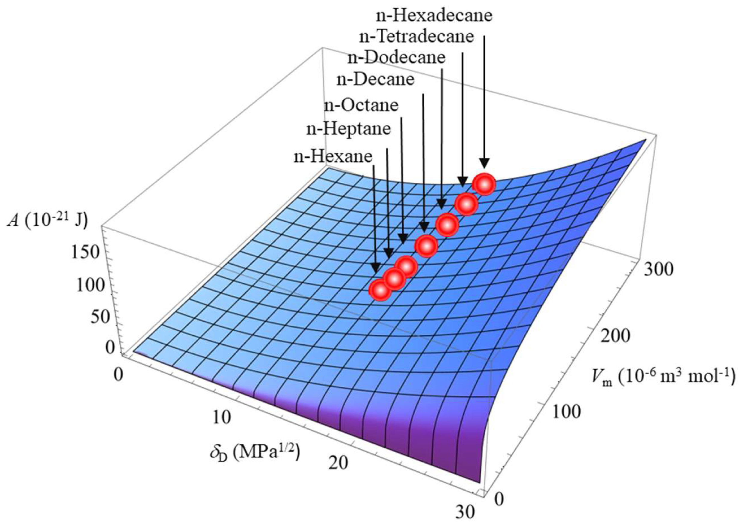
Figure 4 illustrates how the Hamaker constant A depends on δ_D and V_m for completely non-polar liquids with δ_P = 0 and δ_H = 0. The seven small spheres lying on the three-dimensional curved surface in Figure 4 correspond to the seven non-polar liquids, that is, n-Hexane, n-Heptane, n-Octane, n-Decane, n-Dodecane, n-Tetradecane, and n-Hexadecane. Any non-polar liquid may be expressed as a point lying on this three-dimensional surface. On the basis of Figure 4, one can thus predict the precise value of the Hamaker constant of a substance, the value of which is not available.

4. Conclusions

The purpose of the present paper is to bridge quantitatively the Hansen solubility parameter δ, which is one of the key factors in solution chemistry, and the Hamaker constant A, which is one of the key factors in colloid and interface science. The principal result of the present paper is Equation (15) (or Equation (16) for completely non-polar liquids) for the relationship between the Hamaker constant A and the Hansen solubility parameters δ_D, δ_P, and δ_H for non-polar liquids. The Hamaker constant A plays an essential role in determining the stability of colloidal suspensions, and one needs the values of the Hamaker constant to evaluate the stability of colloidal suspensions. The precise values of the Hamaker constant can be estimated based on the rigorous Lifshitz theory [2,3]. This estimation, however, requires laborious numerical calculations involving numerical data on the frequency-dependent dielectric permittivity of substances. In the present paper, we provide a simple expression (Equation (15)) for calculating the Hamaker constant for non-polar liquids based on the Hansen solubility parameters δ (δ_D, δ_P, and δ_H) on the basis of the database of the Hansen solubility parameters [9,10] and the molar volume V_m of the substance molecule, avoiding difficulties associated with the rigorous Lifshitz theory.

In the present paper, we propose a new method for calculating the Hamaker constant A of nonpolar liquids. With the help of the values of the Hamaker constant A of a non-polar liquid, one can calculate the Hamaker constant for the van der Waals interaction between two colloidal particles dispersing in this non-polar liquid based on the following relation:

$$A_{121}={\left(\sqrt{A_1}-\sqrt{A_2}\right)}^2$$

(17)

where A₁ is the Hamaker constant for the van der Waals interaction between these two colloidal particles across a vacuum and A₂ is that for the interaction between the two non-polar liquids across a vacuum.

References

- Hamaker, H.C. The London-van der Waals attraction between spherical particles. Physica 1937, 4, 1058–1072. [Google Scholar] [CrossRef]
- Lifshitz, E.M. The theory of molecular attractive forces between Solids. J. Exper. Theoret. Phys. 1956, 2, 73–83. [Google Scholar]
- Israelachvili, J.N. Intermolecular and Surface Forces, 3rd ed.; Elsevier: Amsterdam, The Netherlands, 2011. [Google Scholar]
- Hough, D.B.; White, L.R. The calculation of Hamaker constnats from Lifshitz theory with application to wetting phenomena. Adv. Colloid Interface Sci. 1980, 14, 3–41. [Google Scholar] [CrossRef]
- Derjaguin, B.V.; Landau, D.L. Theory of the stability of strongly charged and of the adhesion of strongly charged particles in solutions of electrolytes. Acta Physicochim. USSR 1941, 14, 633–662. [Google Scholar] [CrossRef]
- Verwey, E.J.W.; Overbeek, J.T.G. Theory of the Stability of Lyophobic Colloids; Elsevier: Amsterdam, The Netherlands, 1948. [Google Scholar]
- Ohshima, H. Biophysical Chemistry of Biointerfaces; Wiley: Hoboken, NJ, USA, 2010. [Google Scholar]
- Tadros, T.F. (Ed.) Colloid Stability. The Role of Surface Forces—Part 1; Wiley-VCH: Weinheim, Germany, 2007. [Google Scholar]
- Hansen, C.M. Hansen Solubility Parameters: A User’s Handbook; CRC Press: Boca Raton, FL, USA, 2007. [Google Scholar]
- Abbott, S.; Hansen, C.M.; Yamamoto, H.; Valpey, R.S. Hansen Solubility Parameters in Practice, Complete with eBook, Software and Data 4th Edition Version 4.1. 2013. Available online: http://www.hansen-solubility.com/ (accessed on 18 November 2016).
- Tinjacá, D.A.; Martinez, F.; Peña, M.A.; Jouyban, A.; Acree, W.E., Jr. Revisiting the Total Hildebrand and Partial Hansen Solubility Parameters of Analgesic Drug Meloxicam. Liquids 2023, 3, 469–480. [Google Scholar] [CrossRef]
- Fairhurst, D.; Sharma, R.; Takeda, S.; Cosgrove, T.; Prescott, S.W. Fast NMR relaxation, powder wettability and Hansen solubility parameter analyses applied to particle dispersibility. Powder Technol. 2021, 377, 545–552. [Google Scholar] [CrossRef]
- Saita, S.; Takeda, S.; Kawasaki, H. Hansen Solubility Parameter Analysis on Dispersion of Oleylamine-Capped Silver Nanoinks and their Sintered Film Morphology. Nanomaterials 2022, 12, 2004. [Google Scholar] [CrossRef] [PubMed]
- Beerbower, A. Surface free energy: A new relationship to bulk energies. J. Colloid Interface Sci. 1971, 35, 126–132. [Google Scholar] [CrossRef]
- Koenhen, D.M.; Smolders, C.A. The determination of solubility parameters of solvents and polymers by means of correlations with other physical quantities. J. Appl. Polym. Sci. 1975, 19, 1163–1179. [Google Scholar] [CrossRef]
- Pereira, C.N.; Vebber, G.C. A relationship between the heat of vaporization, surface tension, and the solubility parameters, which includes the ratio of the coordination numbers, based on Stefan’s rule. Polym. Eng. Sci. 2019, 59, E312–E321. [Google Scholar] [CrossRef]
- Murase, M.; Nakamura, D. Hansen solubility parameters for directly dealing with surface and interfacial phenomena. Langmuir 2023, 39, 10475–10484. [Google Scholar] [CrossRef] [PubMed]
Figure 1.
The van der Waals interaction between two colloidal particles resulting from the van der Walls interaction between molecules in particle 1 and those in particle 2.
Figure 2.
The surface tension γ, the wok of cohesion 2γ, and the decrease in the van der Waals dispersion interaction energy V(hmin) between two cylinders due to their contact at h = hmin.
Figure 3.
The interaction between two parallel plates 1 and 2 at separation h, whose minimum value, i.e., the closest plate separation, is denoted by hmin.
Figure 4.
The dependence of the Hamaker constant A of completely non-polar liquids with δP = 0 and δH = 0 depending on the dispersion component of the Hansen solubility parameter δD and the molar volume Vm.