The governing differential equation for the voltage (
u) in a body with conductivity distribution
under the spatial coordinates
is given by the following steady state diffusion equation and associated boundary conditions [
1,
28]:
The first boundary condition expressed in Equation (
2) relates the current density over the
electrode (surface) to the electric current
passed through the electrode (
is the outward unit normal) defined by the surface integral over the electrode (
) on the boundary
. The second boundary condition expressed in Equation (
3) specifies the electrode-free insulated boundaries (regions not included in the boundary
). In orthotropic CFRP composites, the conductivity
varies in each layer due to ply orientation, and delamination within the laminate introduces free surfaces within the domain.
2.1. Finite Element Model
The governing equations for the electric potential distribution in a composite laminate with orthotropic plies were solved using ANSYS [
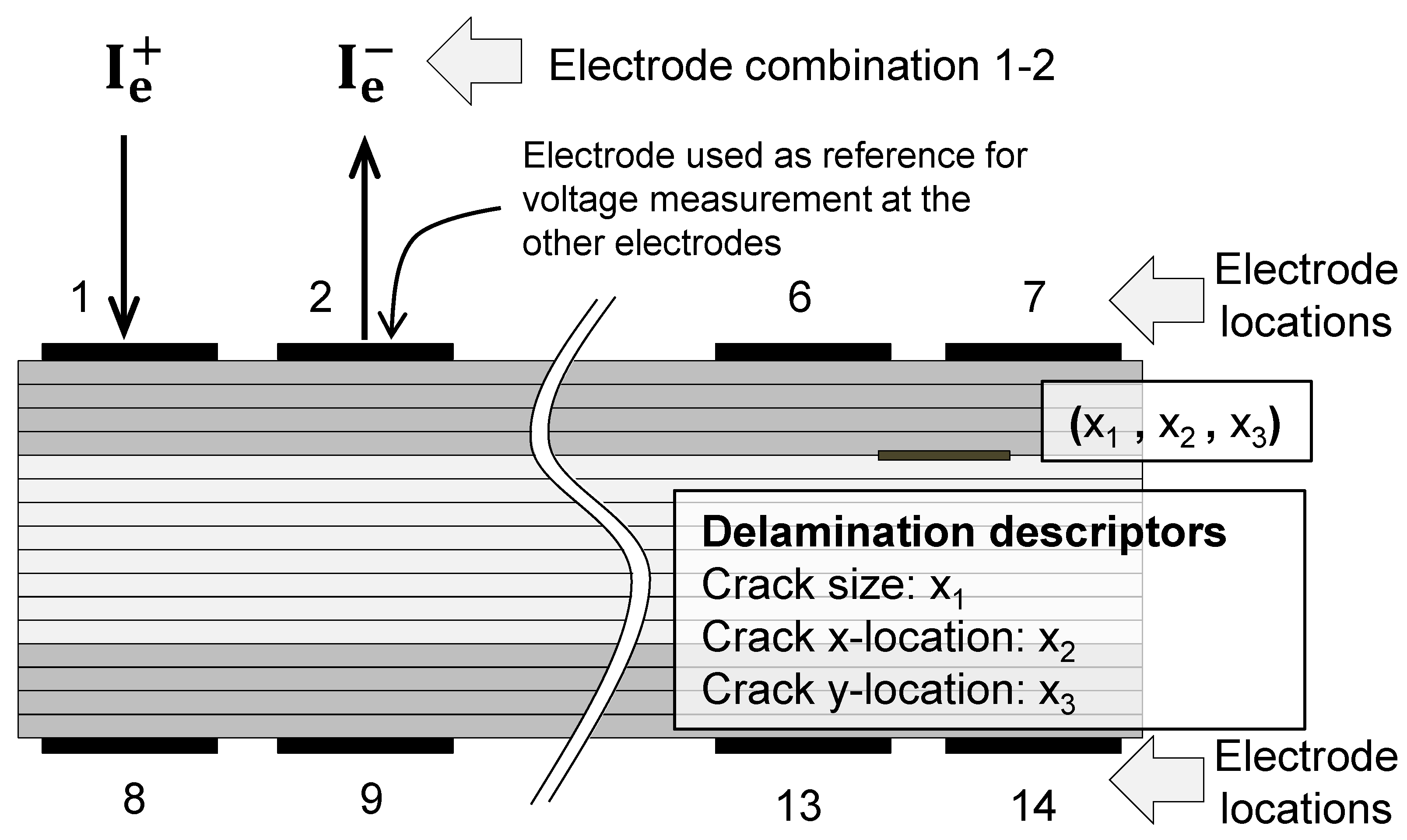
29] FEA softwar (Academic Research, Release 15.0.7, Canonsburg, PA, USA). A simplified 2D planar model for the laminate cross-section that spans the thickness and length of the laminate is analyzed under a specified current injection to obtain the voltage distribution (
Figure 1). The specimen, electrodes and the embedded delamination are all assumed to span the entire depth in the out of plane direction.
A layerwise model is used to analyze 16-ply laminates with and without delamination crack damage. Delamination cracks were created as free surfaces using doubly-defined nodes at the crack interface. The domain mesh consisted of eight node quadrilateral planar electric elements (PLANE 230). A mesh convergence study was performed and the element mesh size was found to be 0.125 mm, which completely spans through the thickness of each ply. This resulted in a model with 27,044 elements.
Orthotropic electrical properties were used [
11] to model
and
cross-ply laminates. The conductivity values used for CFRP correspond to a graphite epoxy composite lamina with 62% fiber volume fraction [
9]. The electrode material (silver) was modeled as isotropic with a 62.9 × 10
6 S/m conductivity.
2.2. Measuring Schemes
In ERT based detection, in general, there are multiple surface electrodes. The schemes for measurements refer to location of the electrode pairs for passing electric current and the locations of the electrode pairs for voltage sensing, relative to the chosen current electrodes. In this section, we discuss the geometric arrangement for the electrode locations corresponding to various schemes such as two, four and multi-probe schemes, and describe the geometric arrangement for the electrode locations.
In a general electrode setting, a specified current is injected between a chosen pair of electrodes and voltages at electrodes can be measured. In this study, the method will be demonstrated using a 2D plane representation of a laminate with electrodes distributed on the top and bottom surfaces of the laminate. This results in a total of possible electrode pairs for passing current.
When the electric potential (
V) is measured between the same electrode pairs through which the electric current (
I) is applied, then this is referred to as a
two-probe (
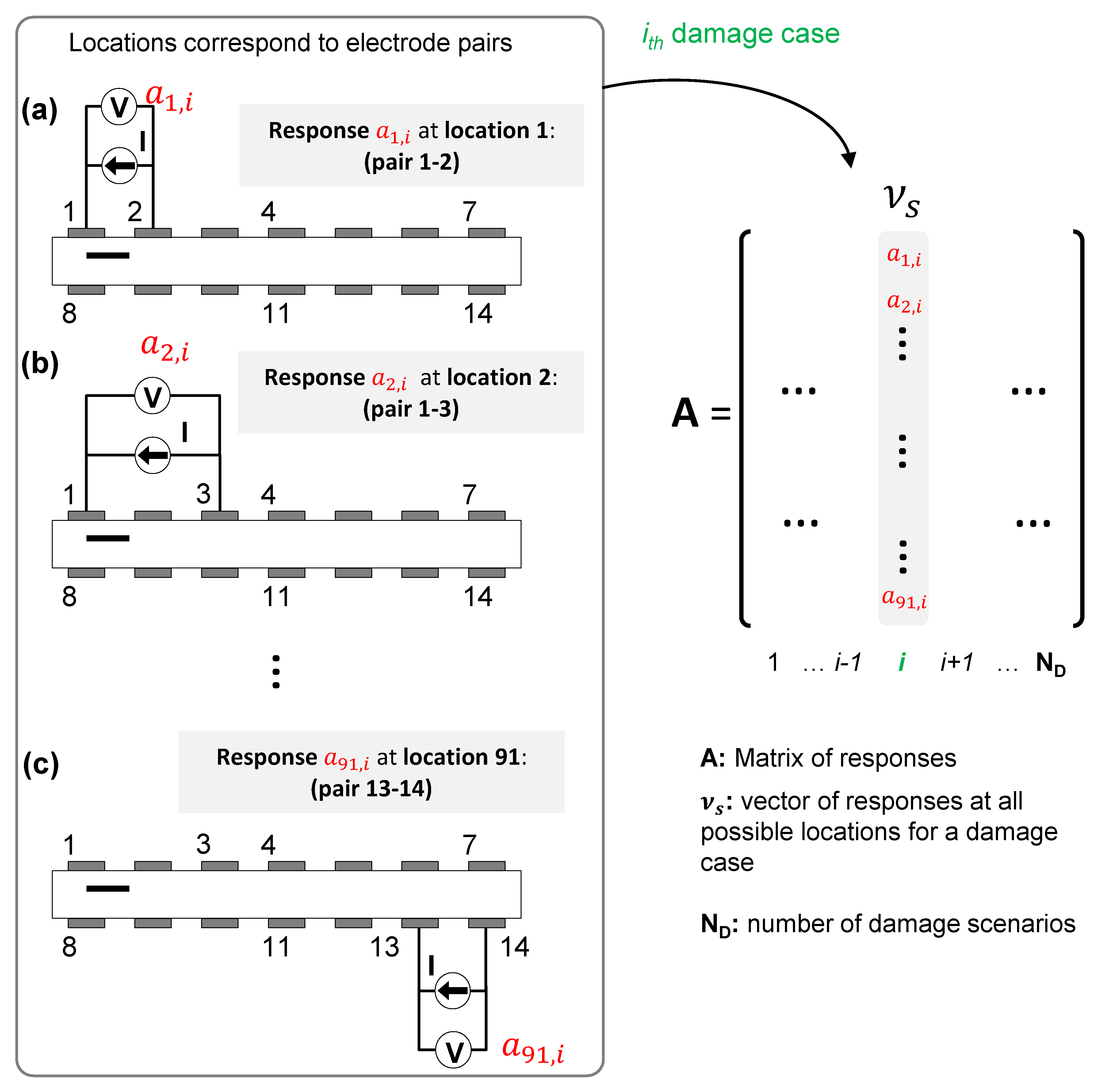
Figure 2). The effective resistance is then computed using Ohm’s Law as the ratio
[
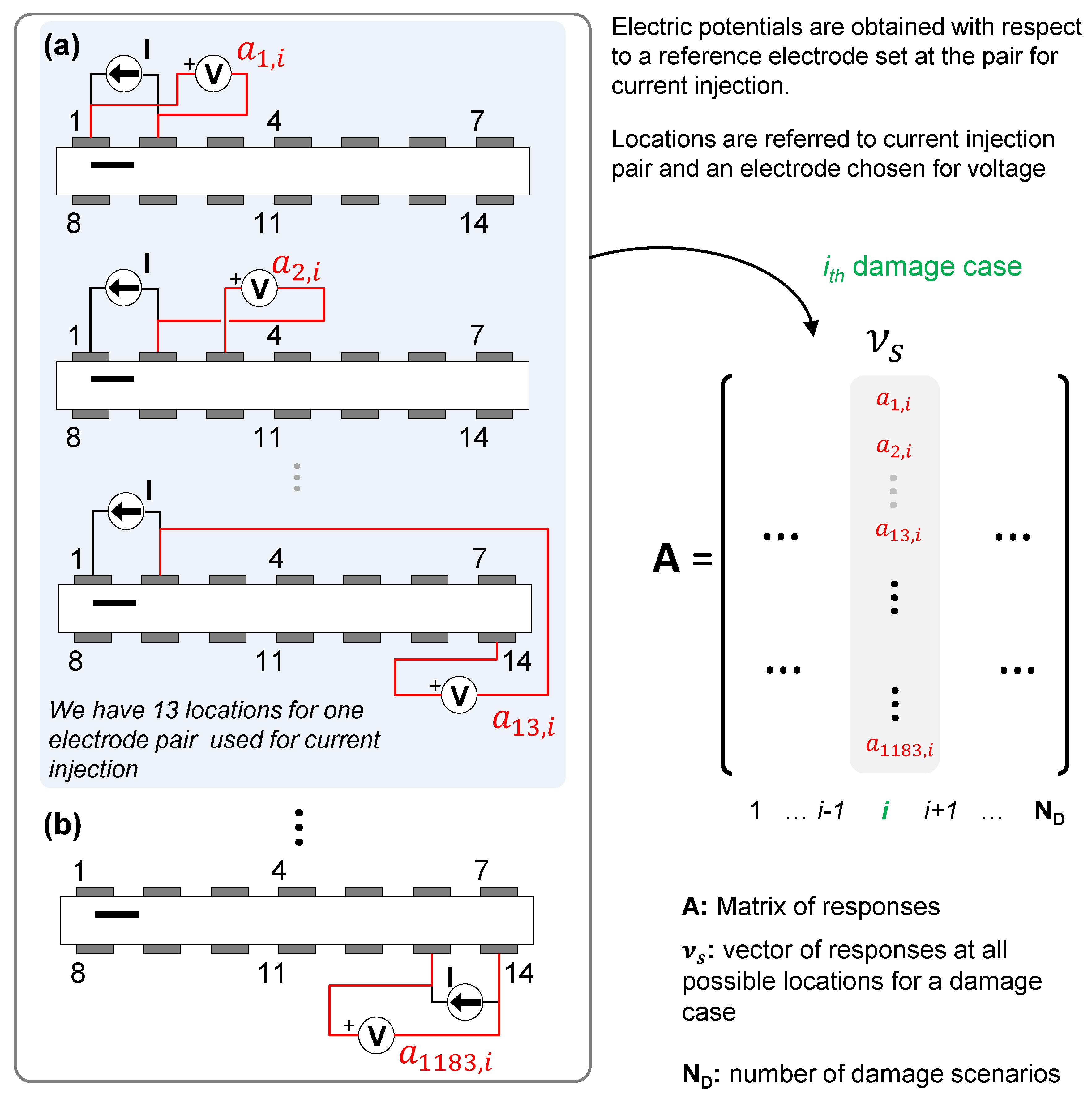
9]. For a given damage case, the voltages measured at all possible electrode combinations are grouped as a vector, hereafter referred to as responses (
). The matrix A shown in
Figure 2 is the collection of responses corresponding to
different damage cases.
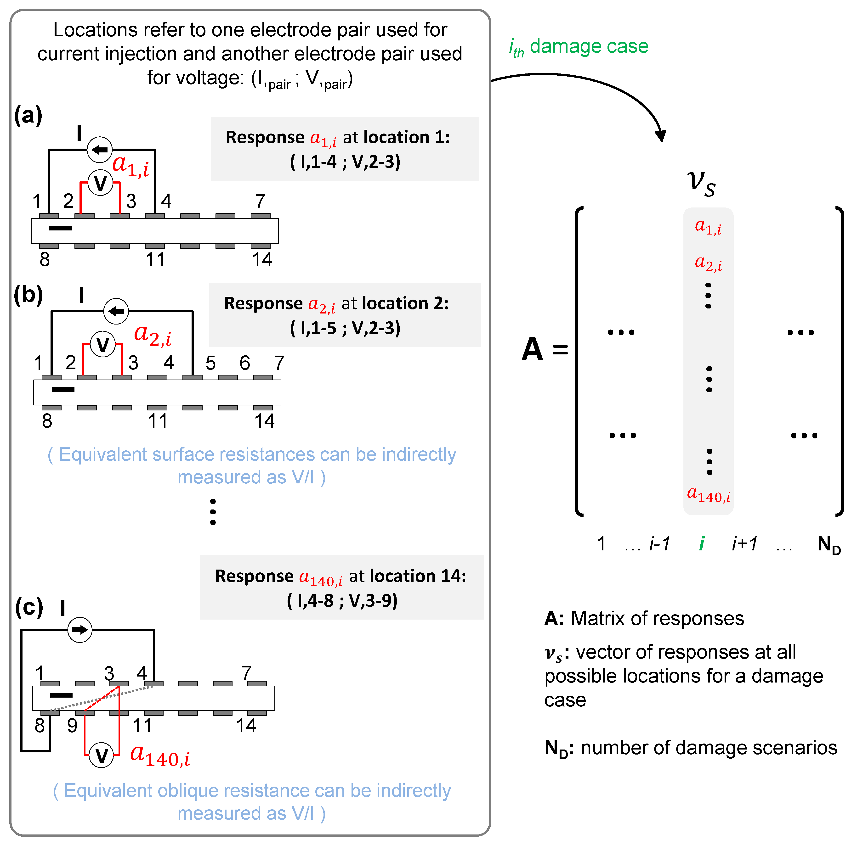
If the electric potential
V is measured at a pair of electrodes that are physically located between the electrode pairs used for current injection (
Figure 3), then this is referred to as a
four-probe [
12]. The ratio of the voltage measured at the electrode pair to the current injected can provide resistance
[
8]. In the four probe scheme, the electrodes for voltage measurements are always located within the physical horizontal space between the two current electrodes. When the two current electrodes are on the same side as in
Figure 3a, then the voltage electrodes are also kept on the same side. When electric current and voltage are measured on the same face, we refer to this as surface resistance (
Figure 3a,b). For example, when the current electrode pair is 1–5 (as in
Figure 3b), the possible choices for voltage electrode pairs are 2–3, 3–4, and 2–4. The larger spacing between electrodes for voltage measurements can sense changes farther away from the surface. When two current electrodes are selected to be on opposite faces, then the voltage measurements’ electrodes are also selected on the opposite faces, but within the range of the current electrodes. For example, if the current electrodes are chosen to be 4 and 8, then possible choices for voltage measurements are 2–10 and 3–9. When current injection and voltage measurement follow a diagonal path, we refer to this as equivalent oblique resistances (
Figure 3c).
For each of the
current electrode injection pairs from the total set of electrode pairs, we can measure electric potentials at
sites with respect to one of the current electrodes used as a reference electrode (
Figure 4). This scheme is referred to as the
multi-probe method [
4].
The total number of possible measurements using the measuring schemes on a composite laminate with a total of
h electrodes distributed either on one side or both sides are summarized in
Table 1.
The goal of this paper is to present a method for optimal selection of electrode pairs for current injection and voltage measurements to perform ERT.
2.3. Effective Independence Based Electrode Selection
This section presents a brief overview of the EI measure and its implementation for electrode selection. The use of EI measures has been previously demonstrated for optimum placement of sensors (accelerometers) for measuring structural vibration modes [
30,
31].
Let
be the measured responses at all possible locations. A modal representation of
is given in terms of matrix
of modal vectors and the vector
of target modes by:
When performing tests, we have measurements of the response at finite sample points from which the modal coefficients have to be estimated. The measurements usually also have some noise, denoted here as
N. The responses at measurement sites
can be expressed using the modal representation, with modal vectors restricted to sensing sites
, as shown in Expression (
5):
If we can assume the responses measured at sampling sites
have uniform and uncorrelated Gaussian noise
N with with variance
, the covariance matrix of estimation errors for the target mode response
from the measured responses
, is obtained by the expected value (
E) in Expression (
6) [
30]:
Minimizing the above covariance matrix is equivalent to maximizing the determinant of the Fisher Information Matrix (FIM) (
Q) leading to the best estimate
. In the case where measurement noise is uncorrelated with identical statistical properties, the FIM can be expressed analogously as
[
30] in Expression (
7):
In the expression above,
corresponds to the
row in matrix
. Deleting a row in
is equivalent to eliminating a sensor location and it removes information from the equivalent FIM [
31]
. The determinant of the new FIM (
) after deleting the
row can be expressed in terms of the original FIM [
31]:
where
is the contribution of the removed sensor to the independent information of
. The contribution of each sensor derived from the eigenvalues and eigenvectors of matrix
Q [
11]. The ranked vector of eigenvalues
provides the Effective Independence values. This effective independence distribution vector
is the main diagonal of the effective independent (EI) matrix
E in Expression (
9):
The computed EI values allow us to rank the sensor locations. After the sensor location with the lowest EI value is eliminated, the vector is recomputed and then iteratively used to eliminate the sensor location with the lowest contribution.
In this paper, we use the EI based method to investigate optimal selection of electrode pairs for the three schemes discussed. The selection requires a numerical model of the forward solution for the electrical conduction problem for the domain of interest. For our demonstration problems, voltage responses were obtained numerically from finite element analyses. The first step of the process is to construct a modal representation of the voltage responses. This is performed numerically. A set of preselected 810 delamination cases obtained from a full factorial (FF) Design of Experiments (DOE) by varying the three variables, namely crack length, crack center location along the
x-axis and crack location along the
y-axis. Since delamination cracks in composites are at interply locations, this variable is discrete. A matrix of responses
is obtained from the numerical simulations. These numerical simulations are then used to obtain the modal matrix
that provides the orthonormal basis for the response
using a Singular Value Decomposition and dimension reduction on
[
11]. Once the modal matrix or orthogonal basis
is available, one can proceed to calculation of the Effective Independence (EI) measures.
With the EI measures obtained from , measurement reduction consists of eliminating the row from with the lowest EI value. The reduction process is performed iteratively by computing the values and updating the matrix by eliminating the row associated with the sensing location with the lowest EI. The termination criteria can be set as given a number of sensors or measurements retained or when the determinant of is less than a threshold value (between and ).
In essence, the EI based selection scheme starts with the complete set of all possibilities and eliminates sites with low contribution until the desired set is obtained.
Since the process of iteratively computing the equivalent FIM for EI based selection implies computation of matrix inversion of the FIM, the condition number of this matrix must be monitored during the process of row elimination from matrix . The initial condition number of the FIM was 1 for all studied cases. After applying the EI based reduction on the different schemes and layups, the condition number increased to a maximum of 13 with a typical final value below 10. This results show that small numerical error is expected from the EI based reduction process.
2.4. Electrode Combinations Reduction
In this section, we will discuss the results of the EI based selection of electrodes of the three measurement schemes (two-, four- and multi-probe) discussed previously. For each case, the optimal electrodes for one-sided and two sided placements of electrodes are discussed. The technique is demonstrated for two crossply laminate designs, one with blocked plies
and the other with distributed plies
.
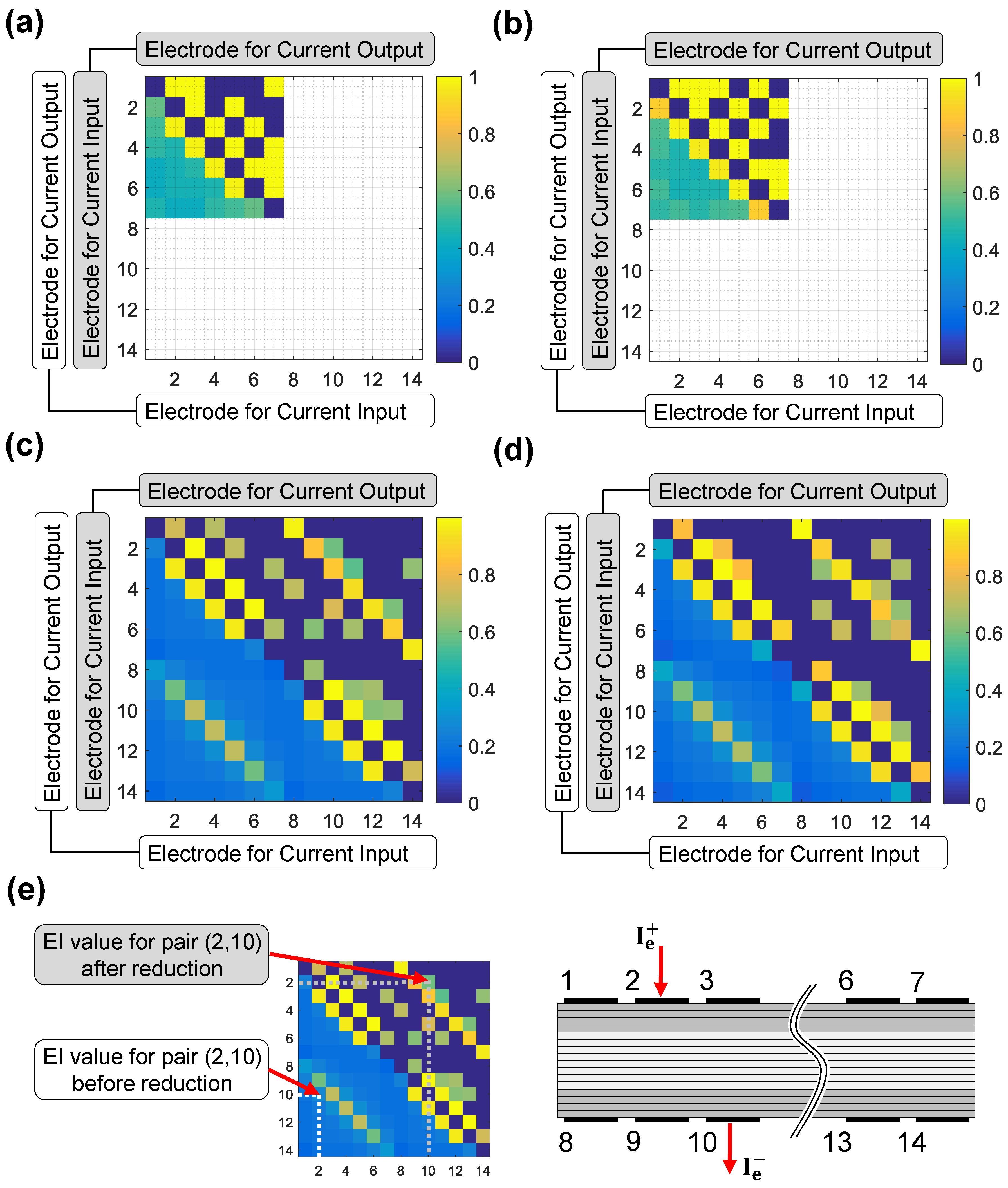
Figure 5 presents the results for the two-probe scheme. The results for electrode selection are summarized by a heatmap plot. The heatmap plot is a 14 × 14 colored grid that represents the values of EI measures for the electrode combinations before and after EI based electrode reduction. The lower triangle of the square grid shows the EI measures for the current electrode pairs (rows)-voltage electrode pairs (columns) for the full set of electrodes. The diagonal and upper triangle of the grid represents the EI of the optimal set of electrodes after EI based reduction. The EI values of the omitted electrode pairs are set to zero.
Figure 5a,c show the results of the retained electrodes under the two-probe scheme for the
laminate for one-sided and two-sided electrodes, respectively. For the two-probe method, using an EI based selection on this stacking sequence resulted in a reduced set with 12 out of 28 electrode pairs for the setting with one-sided electrodes and a reduced set with 34 out of 91 pairs for the setting with two-sided electrodes.
Figure 5b,d show the results of the retained electrodes under the two-probe scheme for the
laminate for one-sided and two-sided electrodes, respectively. When sensor selection is applied on this stacking sequence, a reduced set with 13 out of 28 electrode pairs was obtained for the setting with one-sided electrodes and a reduced set with 32 out of 91 electrode pairs for the setting with two-sided electrodes.
For both layups using the two-probe scheme, the full sets of combinations show that consecutive electrodes (e.g., 1–2, 2–3, 3–4...) have the highest contributions for both one and two face electrode placements. These combinations are preserved in the reduced sets. In the case of 14 electrodes, electrode pairs with vertically opposed placements also show high contributions before and after reduction.
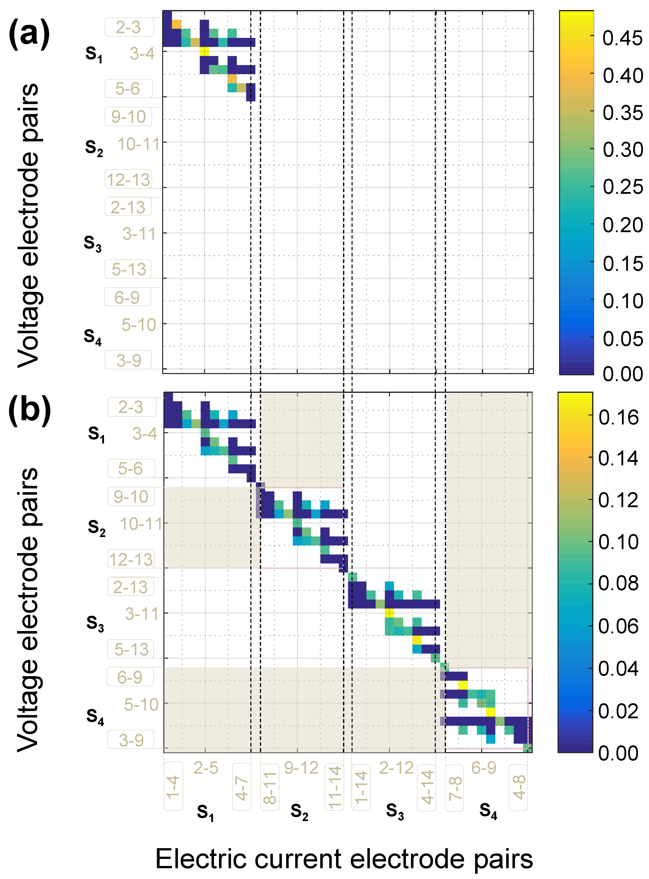
Figure 6 and
Figure 7 show the EI values for the reduced and optimum set of responses for all possible electrode pairs (abcissa) and the corresponding feasible voltage pairs available under four-probe scheme (ordinate). To provide more clarity of the optimal set, the electrode pairs are grouped by their position:
—same side on top surface,
—same side on bottom face,
—opposite faces with oblique left-to-right, and
—opposite faces with oblique right-to-left pairs. All possible combinations have a color on the heatmap. As in the previous case, the EI values of eliminated electrode pairs are set to zero (shown in dark blue).
For the four-probe method, the voltage sites are restricted to lie between the current injection sites. Furthermore, the current injection site itself is not used as a voltage site. This reduces the number of possible combinations. The possible combinations are marked by color on the plots (
Figure 6 and
Figure 7).
Using four-probe schemes on the
laminate results in a reduced set with 13 out of 35 electrode combinations for one-sided electrodes (
Figure 6a) and a reduced set with 55 out of 140 combinations for two-sided electrodes (
Figure 6b). For the one-sided setting, the retained optimal electrode pairs correspond to pairs with the largest separation. However, the highest contribution is found for the electrode pairs with the lowest separations between current injection electrode pairs and voltage pairs. For the two-sided setting, the preserved combinations are associated with evenly distributed groups of surface and oblique resistance with the highest contributions in the latter (e.g., sections
and
in
Figure 6b).
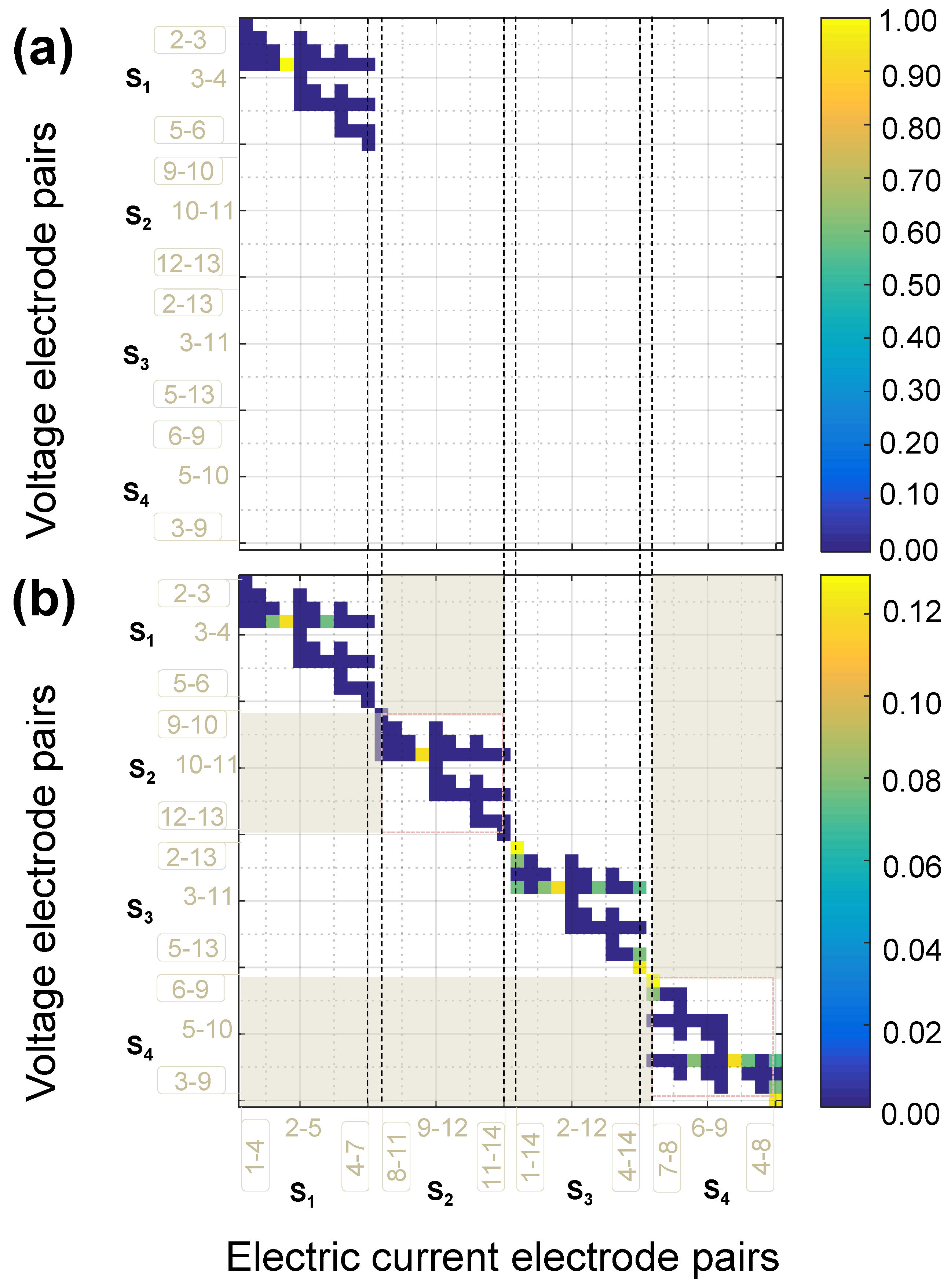
For the
laminate under four-probe schemes, when using one-sided electrodes, only one combination is retained. This corresponds to the electrode pairs with the highest separation for current injection and voltage measurement. When using two-sided electrodes, 21 of 140 combinations are retained. The retained electrode pairs with highest contributions correspond to the oblique pairs
and
(
Figure 7b).
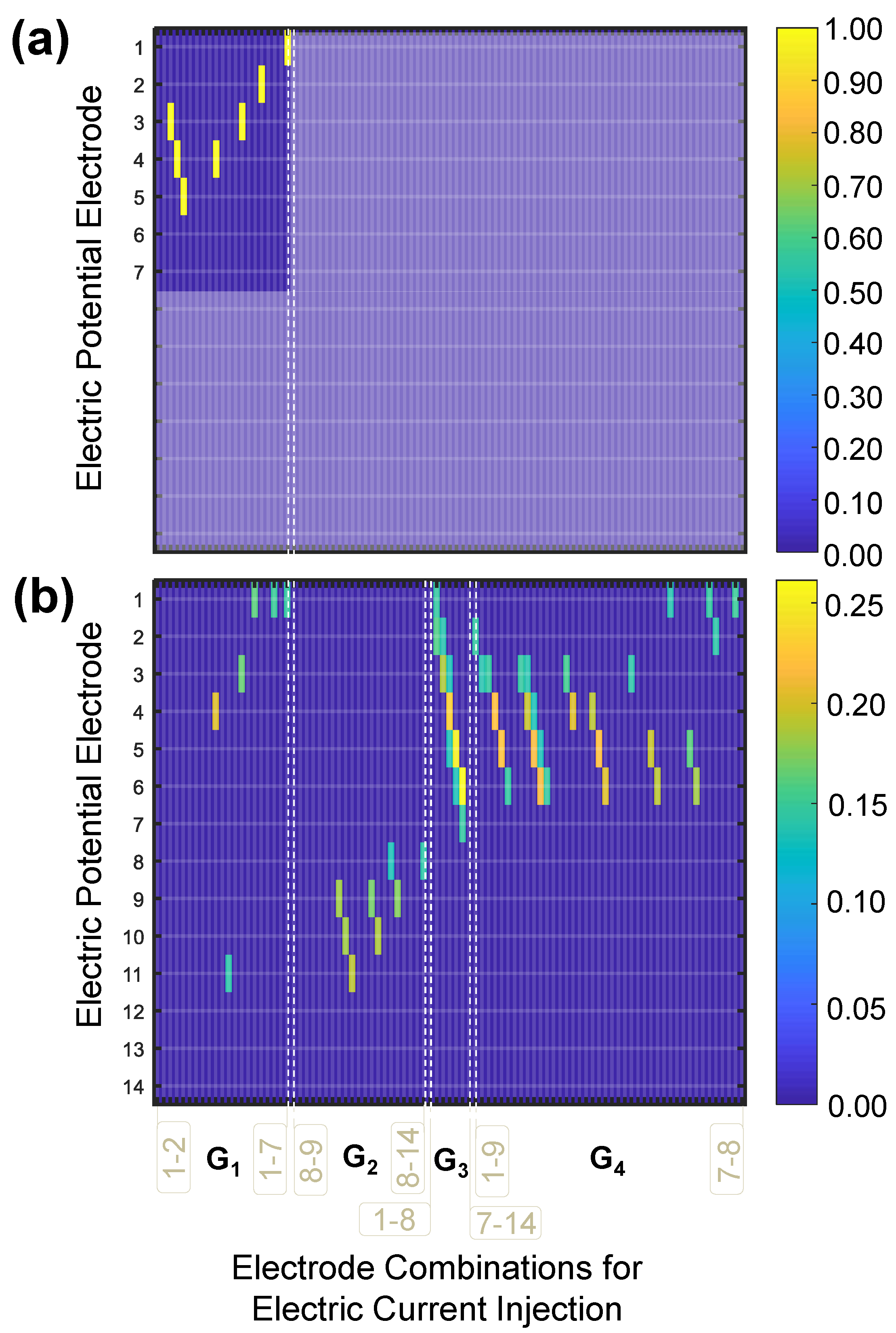
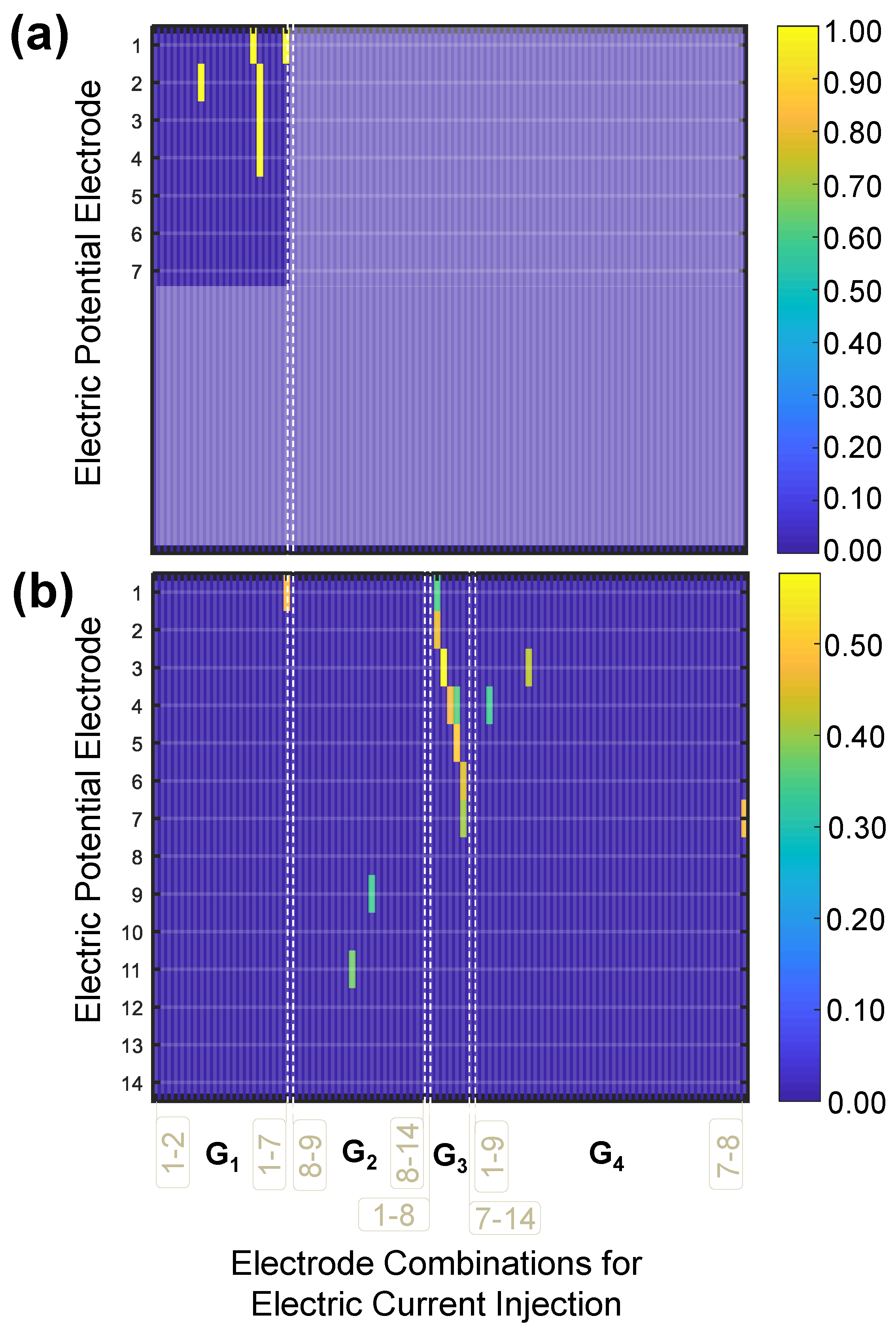
Figure 8 and
Figure 9 show the EI values for the reduced and optimum set of responses using a multi-probe scheme. The results are summarized in a 91 × 14 grid heatmap plot, with the current injection sites along the abcissa and the voltage electrodes along the ordinate axis. The retained combinations for one-sided electrodes are shown in
Figure 8a and
Figure 9a and the retained combinations for two-sided electrodes are shown in
Figure 8b and
Figure 9b. In the EI heatmap plots, the electrode pairs used for current injection are arranged into four major groups:
with electrode pairs on the top surface,
with electrode pairs on the bottom surface,
with electrode pairs facing perpendicularly across the thickness and
with electrode pairs in opposite surfaces facing obliquely. Within each group, the electrode pairs are arranged by the horizontal distance between them in ascending order. This means that, in the
category, the electrode pairs next to each other (1–2, 2–3, 3–4, 4–5, 5–6, 6–7) go first followed by (1–3, 2–4, 3–5, 4–6, 5–7) and so on until the last 1–7 pair. This is also followed for the
group. In the
oblique group, the first half are electrode pairs with top left to bottom right orientation arranged in increasing order of horizontal distance between electrodes, and the second half is the top right to bottom left orientation pairs also arranged in increasing order of distance between the electrodes.
Electrode combination reduction on the multi-probe schemes using one-sided electrodes retains seven out of 126 combinations for the laminate, and six out of 126 combinations for the laminate are retained using one-sided electrodes. For both layups, the retained combinations were those in which electric potential is measured at the electrode where electric current is injected, which is equivalent to a direct resistance measurement (as in a two-probe scheme).
Electrode combination reduction in multi-probe schemes retains 53 out of 1183 combinations for the laminate and 14 out 1183 combinations for the laminate, with two-sided electrodes. In both layups, most of the retained combinations were also those related to direct resistance measurement. These oblique resistance measurements were found to have the largest contributions in the multiprobe scheme with two-sided electrodes.
2.5. Inverse Identification Accuracy with Electrode Selection
To assess the effectiveness of the EI based sensor selection, we perform inverse identification with the full set and the EI based optimal selected set of electrodes. The inverse identification procedure used is based on a surrogate based optimization approach previously demonstrated successfully for ERT problems by the authors [
11,
32]. In this procedure, we minimize computational effort by fitting a Kriging surrogate model to the voltage responses obtained by a FEA model. The responses obtained for damage cases created using a full factorial design of experiments (810 cases) by varying crack size, and crack
x- and
y-locations were used in the Kriging model fit. This eliminates the use of a FEA model in the inverse identification optimization directly. A separate set of 40 test cases derived from a Latin Hypercube Sampling (LHS) DOE of the damage variable space was analyzed using FEA to obtain the needed voltage/resistance responses. These responses are used in lieu of test data as synthetic test data to see how well the inverse optimization can identify these damage cases. The optimization minimizes the
of the difference between the synthetic responses (simulated measurements) and the predicted responses (from the surrogate). Note that the surrogate Kriging model can introduce a small modeling error, so model and synthetic data can differ even at the same points. The RMS value of the leave one out cross validation errors for the Kriging model were of the order of 5% or less [
32]. The max local errors were of the order of 10%. The inverse optimization does not use any regularization as it only has a small number of variables (the crack parameters), unlike ERT where the description of the entire conductivity field is used as the design variables. Global optimization with Genetic Algorithms (GA) is used.
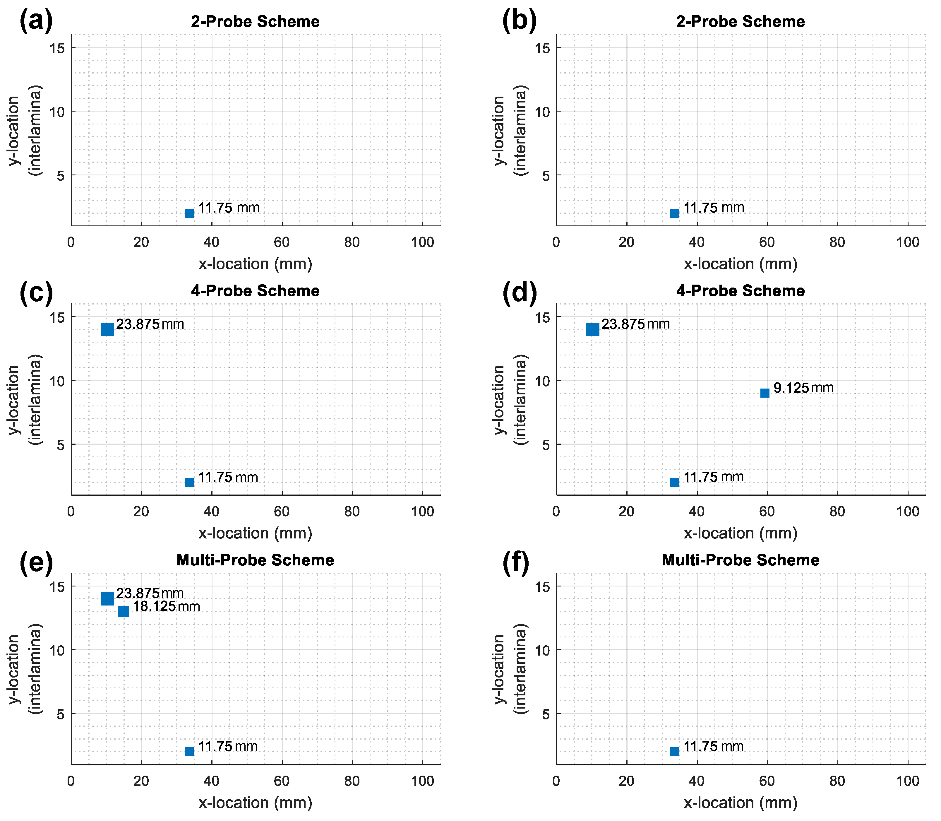
The accuracy of the inverse identification on 40 test cases for the full set of electrode measurements and reduced set for all three measuring schemes is summarized in
Table 2. Each test case uses three damage descriptors, namely: size,
x-location and
y-location. The inverse identification predicts the value at each descriptor for every test case. The relative error (RE) between the actual (
) and the predicted (
) value at each damage descriptor is computed and the maximum relative error obtained is used to assess the inverse identification accuracy for a given test case according to Equation (
10):
The RE for crack size are calculated relative to the electrode center to center spacing equal ( mm). The RE for the horizontal spacing are calculated relative to the range of used for the DOE points ( mm). The RE for vertical location are computed relative to the total number of plies (). The Root Mean Square (RMS) of the maximum relative errors between the damage descriptors and their predicted values found by inverse identification for the 40 cases is computed.
In addition, the number of cases with relative errors in inverse identification that were larger than 10% are considered as failed cases. The total number of failed cases and the computed RMS values at each set using the specified scheme and setting shown in
Table 2 are used for comparison.
2.5.1. Two-Probe Schemes
The results for the layup using the two-probe scheme with one-sided electrodes show that, for the full set of measurements, out of the 12 failed cases, 100% are associated with error in crack size identification. However, crack y-location identification also fails for 83.33% of these cases with an average error magnitude of approximately 13% equivalent to the resolution for 2-ply. For the reduced set of measurements, 90.1% of the 11 failed cases are associated with error in crack size identification, whereas the remaining 9.9% are associated with error in crack y-location identification. However, error in the crack location identification is also larger than 10% in 72.7% of the failed cases with an average error magnitude of 15.6% equivalent to the resolution of 2-ply.
The two-probe scheme on the
layup with two-sided electrodes and the full set of measurements results in one failed case associated with error in crack size identification. Besides error in crack size, the largest magnitudes are also associated with error in
y-location identification equivalent to the resolution of 1-ply. For the reduced set of measurements, the only case that fails is associated with error in crack size. The large magnitudes in crack size identification errors are followed by the errors in
y-location identification, equivalent to the resolution of 1-ply. The failed case is the same for both sets (see
Figure 10a,b).
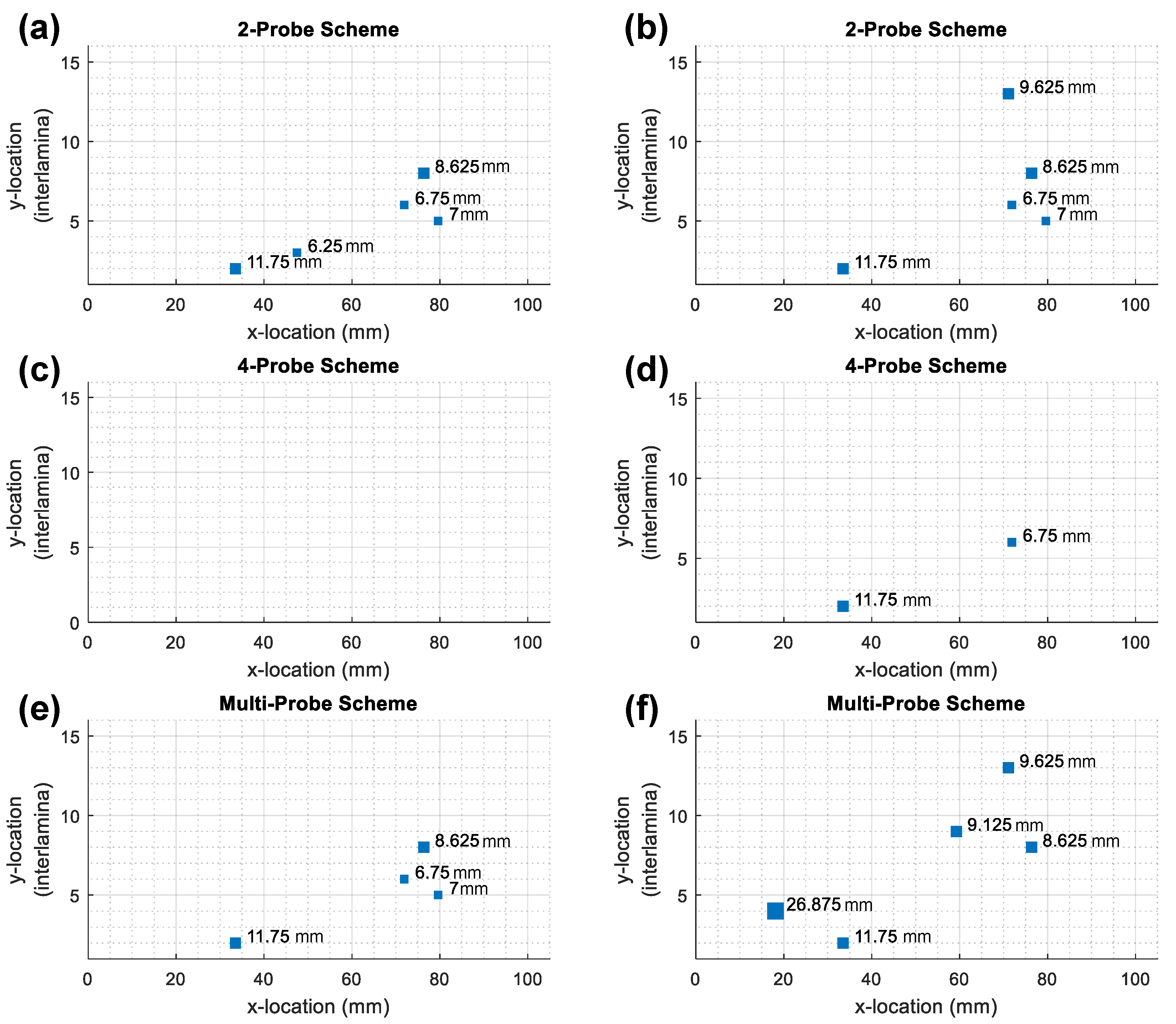
The results for the layup using the two-probe and one-sided electrodes show that, for the full set, 10 cases failed and 80% of them were associated with error in crack size and 20% with error in y-location identification. However, crack y-location identification also fails in 70% of these cases with an average error magnitude of 16% equivalent to approximately the resolution for 2-ply. For the reduced set, 75% of the 15 failed cases are associated with error in y-location identification and 25% with crack size identification. However, crack size identification shows errors larger than 10% in 37.5% of the failed cases with an average error magnitude of 27%.
Using two-sided electrodes in a two-probe scheme on the
laminate has a total of five failed cases out of the total 40 test cases. Of these five cases, two failed cases (40%) correspond to crack size identification and three (60%) failed in
y-location identification. The average error in crack size identification was 13% and the
y-location error equivalent to 3-ply. For the reduced set of measurements, a total of five cases failed. Two out of the five failed cases (40%) are associated with errors in
y-location identification and three out of five failed cases (60%) were for errors in crack size identification. The errors in crack size identification for failed cases were on the order of 17%, while the
y-location errors were on the order of 3-ply thicknesses. The failed cases with one exception were the same for both sets (see
Figure 11a,b).
2.5.2. Four-Probe Schemes
The results of using the four-probe scheme on the layup and one-sided electrodes result in 14 failed cases out of the total 40 test cases for the inverse optimization using the full set of measurements. In these cases, 78.57% (11 out of 14) are associated with identification error in crack size and 21.43% (three out of 14) are associated with errors in y-location identification. Error in crack y-location identification exceeds 10% in 64.29% (nine out of 14) of the failed cases and an average error of 20.14%, approximately equivalent to 3-ply. For the reduced set of measurements, inverse identification failed for 17 cases out of the 40 test cases. Of these 17 cases, 14 cases or 82.35% are associated with large errors in crack size identification and three out of 17 (17.65%) with y-location. For the failed cases, crack y-location identification error exceeds 10% in 76.47% (13 out of 17) of the cases with average error magnitude of 23.08%, which is equivalent to approximately 4-ply.
The four-probe scheme applied on the
layup using two-sided electrodes for the full set of measurements results in only two failed cases among the 40 test cases, both associated with large errors in crack size identification. Errors in
y-location identification were on the order of 1-ply. In the inverse identification with a reduced set of measurements, only three cases out of the total 40 test cases failed. Two failed cases are associated with error in crack size identification and one with error in
y-location identification. The errors associated with
y-location are on the order of 1-ply thickness. The failed cases with one exception are the same for both sets (see
Figure 10c,d). One of the failed cases coincides with the failed case from the two-probe scheme.
Inverse identification using the four-probe scheme on the layup and one-sided electrodes with the full set of measurements results in 13 failed cases among the total 40 test cases. In the failed cases, 53.85% (seven out of 13) are associated with crack size identification errors and 46.15% (six out of 13) are associated with y-location errors. Inverse identification error in crack y-location exceeds 10% in 76.92% (10 out of 13) of the failed cases with an average error of 18.75% equivalent to approximately 3-ply. For the reduced set of measurements, almost all cases fail (39) with 58.97% of them associated with error in crack size and the rest with errors in x-location and y-location.
The four-probe scheme applied on the
layup using two-sided electrodes for the full set of measurements results in no failed cases. Some cases have prediction errors larger than 5% associated with error in crack size and
y-location identification. For the reduced set of measurements, only two cases failed, one is associated with crack size and one with
y-location identification. The failed cases in the reduced set (see
Figure 11d) coincide with two of the failed cases from the two-probe scheme.
2.5.3. Multi-Probe Schemes
Using multi-probe schemes on the layup with one-sided electrodes for the full set of measurements results in 10 failed cases, of which 90% (nine out of 10) are associated with error in crack size identification and 10% (one out of 10 failed cases) with y-location identification. Among the failed cases, crack y-location identification error exceeds 10% in 80% of them with average error magnitude of 18% equivalent to approximately 3-ply. Inverse identification using the reduced set resulted in 12 failed cases, of which 83.33% are associated with errors in crack size identification and 16.67% with errors in y-location identification. The crack y-location identification error exceeds 10% in 75% of the failed cases with an average error magnitude of 17.36% equivalent to approximately 3-ply.
Inverse identification with two-sided electrodes on a
laminate with multi-probe schemes using the full set of measurements results in three failed cases. These cases are associated with crack size identification error. Besides crack size, the largest errors found in
y-location identification were equivalent to the resolution of 1-ply. For the reduced set, only one case fails and it is associated with error in crack size identification. The largest errors in
y-location identification are equivalent to the resolution of 1-ply. The failed case in the reduced set also fails for the full set (see
Figure 10e,f). This case corresponds to delamination near the top surface under one electrode and fails for all sets and schemes in this layup.
Using multi-probe schemes on the layup with one-sided electrodes for the full set of measurements results in 16 failed cases, of which 56.25% (nine out of 16) are associated with error in y-location identification and 43.75% (seven out of 16) with crack size identification. Inverse identification with the reduced set of measurements results in 16 failed cases, 68.75% (11 out of 16) are associated with error in y-location identification and 31.25% (five out of 16) with error in crack size identification.
Using multi-probe schemes with two-sided electrodes for inverse identification on the
laminate with the full set of electrodes results in four failed cases out of 40 test cases—of which, two are associated with crack size identification and two with
y-location identification. The largest errors found for
y-location identification are equivalent to the resolution of 1-ply. Inverse identification with the reduced set of measurements results in five failed cases, of which three are associated with
y-location identification and two with crack size. The largest errors below the 10% limit are associated with
y-location identification and are equivalent to the resolution of 1-ply. Two failed cases are found to be common between the complete and reduced set (see
Figure 11e,f). These two cases correspond to damage near the top surface under one electrode and delamination in the horizontal midplane. The failed case near the top surface is common to all the schemes and layups, whereas the case in the midplane is only found in the two-probe and multi-probe schemes.


