2.3.2. Method of Analysis
In the first method, modal parameters, natural frequency (
) and damping ratio (
), are identified using the developed ‘modified peak picking’ approach. ‘Peak-picking’, in the general sense, refers to the usage of graphical features of the real and imaginary parts of the FRF near the natural frequencies to estimate modal parameters [
3,
4,
5]. Different resources may refer to slightly varying formulations of the ‘peak-picking’ method, although they share a similar basic idea. In this paper, a modified approach from traditional ‘peak-picking’ is taken in which the accelerance FRF is employed directly. The derivations of the formulas for this case are presented in the proceeding section side-by-side with formulas that have traditionally been used for receptance. Hence, by avoiding the numerical conversion from accelerance to receptance, the problem of double-integrating the low frequency noise can be largely circumvented through the use of the proceeding modified formulas.
Accelerance FRF between two coordinates (
i and
k) of a proportionally damped multi-degree of freedom (MDOF) system can be presented as a combination of vibratory modes as [
3],
where,
is the number of modes,
and
are the
i-th and
k-th elements of the
r-th mode shape vector,
is the natural frequency,
is the damping ratio, and
is the modal stiffness. In the case of a point FRF (
),
can be set without loss of generality, which makes
equivalent to the static compliance contribution of each mode. The receptance for the same FRF (
) can be obtained from the accelerance as,
Equation (2) can be separated into real and imaginary parts as,
where
represents the normalized frequency. If the modes are assumed to be separated from each other (i.e., having sufficiently distant natural frequencies), the real and imaginary plots of the FRF near each eigenfrequency
(
) would resemble the characteristics of a single-degree-of-freedom (SDOF) system as shown in
Figure 5 for both accelerance and receptance. Note that the extrema of the real and imaginary parts of the accelerance (
,
,
) around the natural frequency (
) attain close but different values than those for receptance (
,
,
), with the difference depending on the damping ratio (
). However, the real part crossing of the abscissa is the same at
for both cases.
Important characteristics of the real and imaginary plots of the FRF, and how they can be used to extract modal parameters (i.e., damping ratio, natural frequency, and modal participation factor) are summarized in the following, including the new steps proposed in our modified peak picking method:
Setting
yields two positive roots as,
and
. Hence, in our approach, the frequency values coinciding with the minimum and maximum real components of accelerance around the natural frequency (
) are used to determine the damping ratio as,
In traditional peak picking, extrema of the real component of receptance are considered, which occur at the following frequencies, leading to the corresponding damping ratio expression,
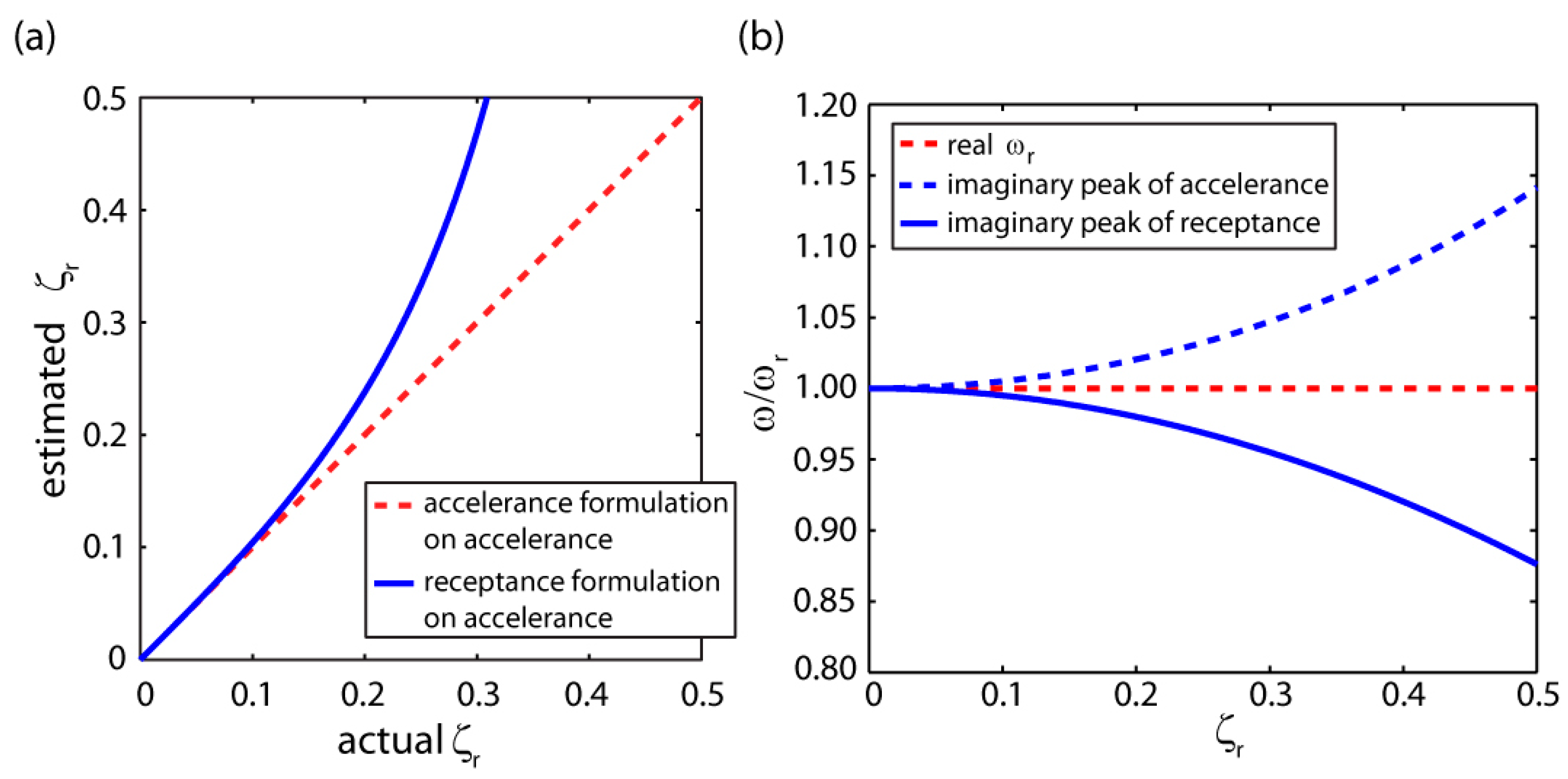
Figure 6a presents a comparison between the damping ratio values estimated from the real component of accelerance. When the proposed formulation in Equation (5) is used, the damping ratio is estimated correctly. However, if the traditional receptance formulation in Equation (6) is applied together with the approximation that
and
, then the damping ratio can only be estimated reasonably well if its actual value is 0.05–0.07 or less. In the case of the actual damping being higher, the use of Equation (6) yields a significant error when peak frequencies of real accelerance are substituted in place of their receptance counterparts. In the comparative modal testing results presented in
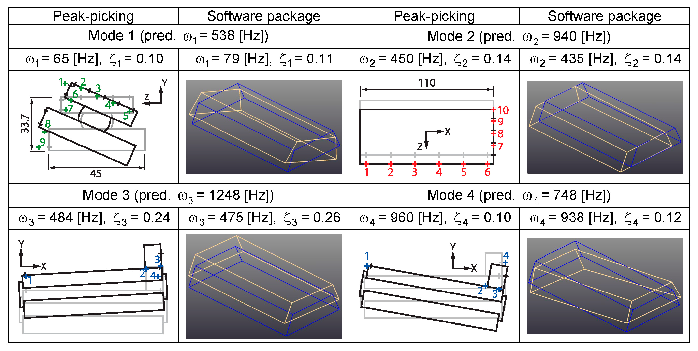
Section 2.6, damping ratios as high as
= 0.24 were encountered, with the vibration modes originating mainly from air bearing/bushing stiffness and damping properties. The receptance formulation in this case would have given incorrect estimates. Hence, the development of separate formulations for accelerance-based peak-picking was an obvious necessity in this study, and can be applied in other systems as well.
- ii.
Setting
yields only
as the positive root. For
,
can be assumed. Hence, the imaginary peak/dip location is used to identify the natural frequency (
). For receptance, the imaginary peak location is obtained as,
In
Figure 6b, estimation of the natural frequency using accelerance versus receptance peak values is shown. It is observed that using the imaginary peak yields similar accuracy in both cases. Also, while the accelerance case overestimates, and deteriorates slightly faster for high values of
, the receptance method underestimates the true
. Overall, both methods are suitable for peak picking to a certain extent for their type of measurement.
- iii.
Limit yields and 0. Hence, real part of accelerance has residues from the lower frequency modes, and using the horizontal axis crossing of for natural frequency estimation would be inaccurate.
- iv.
Limit 0 yields 0 and 0. Hence, in accelerance, higher frequency modes typically do not have an influence on their lower frequency counterparts. In the case of receptance, the situation is reversed in which the higher frequency modes affect the real part only, and lower frequency modes exert very little influence.
For mode shapes to be identified, either the accelerometer location can be fixed and force impacts at different locations can be applied (roving hammer), or the impact location can be fixed while the accelerometer is placed at different points for each measurement (roving accelerometer). Due to the reciprocity rule (), results from the two cases should be equivalent in a linear system. Roving hammer measurements (for the same number of measurement points) can be carried out more quickly, as impacting at a point does not require any significant preparation. On the other hand, in the roving accelerometer case, more time is needed to properly mount the accelerometer at each measurement point, generally using wax. If one wants to determine mode shapes in three dimensions, which allows for a full three dimensional display of the vibratory motions, the response at every measurement point has to be measured in all three orthogonal axes. For the roving hammer case, this requires impacts in three orthogonal directions to be applied at each measurement point. This is very cumbersome; first, due to the difficulty of adjusting the orthogonal impact directions, second, due to the likelihood of some points being impossible to reach from all three directions. In such cases, it is much more advantageous to use a tri-axial accelerometer, which can output accelerations in all three axes at the same time, in roving accelerometer configuration. This way, both the problem of orienting measurement axes is solved, and the possibility of being obstructed by the measured structure is minimized, as the accelerometer is both smaller, and stays in place during measurement. In this paper, as the mode shapes are manually sketched in method 1, roving hammer configuration is used to obtain two dimensional mode shapes using hammer impacts from a single direction for each measurement point. On the other hand, taking advantage of the availability of three dimensional automated calculation and animation of mode shapes, in method 2, roving accelerometer configuration is used with a tri-axial accelerometer.
Denoting the accelerometer location as ‘
o’, the accelerance FRF is given by
. As the imaginary peak/dip approximately occurs at
, the value of the peak/dip (
) can be expressed as:
Value of the imaginary peak/dip measured for a number of impact points,
, can be related to the mode shape (
) as,
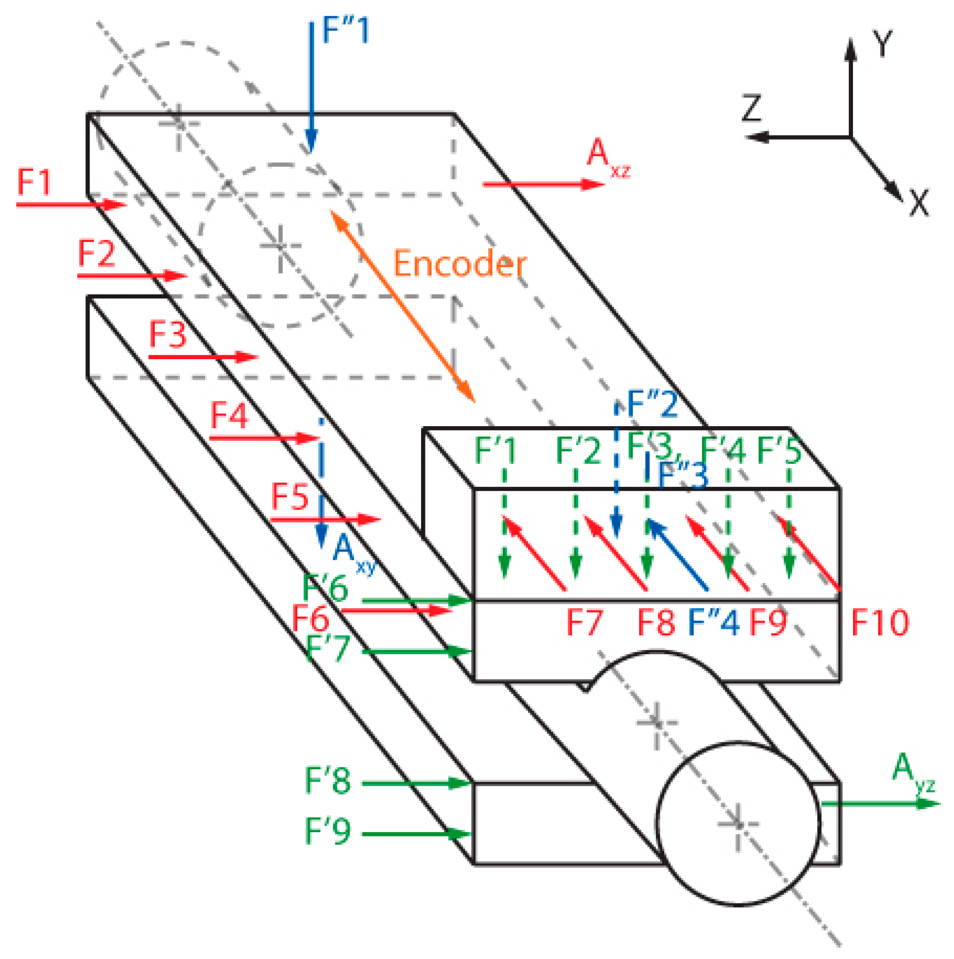
As the mode shapes, which are essentially eigenvectors of the system dynamics, can be scaled by any constant factor, the imaginary peak/dip values can be directly used for visualizing the elements of the mode shape vector. An example case of how the modes are sketched is illustrated in
Figure 7, for the
YZ measurement plane. The values of
can be carried on the undeformed sketch of the structure using a graphical scaling factor. The deformed body is sketched using the displaced points, matching the displacements in their respective axes. For the actual analysis, additional points such as
to
are also considered.


