Article

Large-Scale Reality Modeling of a University Campus Using Combined UAV and Terrestrial Photogrammetry for Historical Preservation and Practical Use

1
Department of Civil and Environmental Engineering, Ira A. Fulton College of Engineering and Technology, Brigham Young University, 368 Clyde Building, Provo, UT 84602, USA
2
Department of Chemical Engineering, Ira A. Fulton College of Engineering and Technology, Brigham Young University, 350 Clyde Building, Provo, UT 84602, USA
*
Author to whom correspondence should be addressed.
Drones 2021, 5(4), 136; https://doi.org/10.3390/drones5040136
Submission received: 1 October 2021 / Revised: 13 November 2021 / Accepted: 14 November 2021 / Published: 17 November 2021

Abstract

:
Unmanned aerial vehicles (UAV) enable detailed historical preservation of large-scale infrastructure and contribute to cultural heritage preservation, improved maintenance, public relations, and development planning. Aerial and terrestrial photo data coupled with high accuracy GPS create hyper-realistic mesh and texture models, high resolution point clouds, orthophotos, and digital elevation models (DEMs) that preserve a snapshot of history. A case study is presented of the development of a hyper-realistic 3D model that spans the complex 1.7 km 2 area of the Brigham Young University campus in Provo, Utah, USA and includes over 75 significant structures. The model leverages photos obtained during the historic COVID-19 pandemic during a mandatory and rare campus closure and details a large scale modeling workflow and best practice data acquisition and processing techniques. The model utilizes 80,384 images and high accuracy GPS surveying points to create a 1.65 trillion-pixel textured structure-from-motion (SfM) model with an average ground sampling distance (GSD) near structures of 0.5 cm and maximum of 4 cm. Separate model segments (31) taken from data gathered between April and August 2020 are combined into one cohesive final model with an average absolute error of 3.3 cm and a full model absolute error of <1 cm (relative accuracies from 0.25 cm to 1.03 cm). Optimized and automated UAV techniques complement the data acquisition of the large-scale model, and opportunities are explored to archive as-is building and campus information to enable historical building preservation, facility maintenance, campus planning, public outreach, 3D-printed miniatures, and the possibility of education through virtual reality (VR) and augmented reality (AR) tours.

1. Introduction

Universities, as centers of learning and development, have contributed greatly to human progression and education through the centuries. Unfortunately, much of universities’ cultural heritage and infrastructure has faded from memory or has only been captured in rudimentary written form, drawings, and/or simple photos. As technology and reality modeling in geomatics has advanced, new ways for preserving campus and university cultural and infrastructural heritage have emerged that revolutionize the level of historical and cultural preservation that is now possible.
A case study of a large-scale 3D model of the Brigham Young University (BYU) campus showcases how photogrammetry can compare with large models made by light detection and ranging (LiDAR) and other techniques that process big data for complex urban and industrial infrastructure scales and details a workflow and best practices for small and large scale SfM model creation. With 80,384 photos and covering a complex 1.7 km 2 area, this case study of the BYU campus in Provo, Utah presents a scaled-up application of unmanned aerial vehicle (UAV) and terrestrial photogrammetry and advanced image data acquisition techniques, captures the historical essence of the campus during the COVID-19 pandemic during the Spring and Summer of 2020, serves as a potential step-out deployment of smart campuses, and leverages heuristics, algorithms, and machine learning in building and analyzing the final 3D model. This model not only serves as a historical campus 3D snapshot, but also becomes a tool that can be used for university construction expansions, 3D-printed miniature recreations (see Section 4.6), and public relations efforts such as providing realistic video renderings and virtual tours of the campus through means of augmented or virtual reality (AR & VR, see Section 4.5) and state-of-the-art visualization software. Growing and enabling technologies allow for additional remote sensing as well as processing of big data in urban environments. The existence of the model potentially allows for improved inspection and maintenance of buildings, masonry, and the campus as a whole. Additionally, algorithms that solve well-known combinatorial optimization problems such as the traveling salesman problem (TSP) and the set-covering problem (SCP) meet up in the use of autonomous UAV photogrammetry and terrestrial photogrammetry in acquiring optimized model data. Emerging processes and applications of machine learning, such as object recognition, permit the case study to reiterate some of the practical applications of these technologies.

2. BYU History, UAV Photogrammetry, and Algorithms

BYU is a campus rich with heritage and an interesting history. Founded by refugee pioneers from The Church of Jesus Christ of Latter-Day Saints, it represents one of the earliest higher education institutions started in Utah and the United States Mountain West region.
This unique campus history began when Brigham Young Academy was founded in 1875 through a Deed of Trust drawn up by Brigham Young and dated the ’16 of October’. According to The Brigham Young University Press, on 11 November 1875, the Deed of Trust was notarized in Salt Lake City, Utah, formally starting Brigham Young Academy. While the Deed of Trust had been signed and notarized, Brigham Young Academy did not open until 3 January 1876 because there was no physical location. The first home of Brigham Young Academy was the Lewis Building on 3rd West and Center Street of Provo, Utah. In late January of 1884, the Lewis building burned down by a fire of unknown cause. After much financial struggles, a new ’Academy’ (building) was completed in the Fall of 1891 [1].
From the inception as Brigham Young Academy in 1875 to the school becoming a university on 23 October 1903, campus buildings and infrastructure inexorably tie into to BYU’s success [2]. Over 146 years, around 300 buildings have been cataloged on the university’s 560 acres [3]. The Brigham Young Academy was built in 1891 and the 19,255 square foot Karl G. Maeser building (MSRB) was built in 1911 as the first permanent building on “upper campus” (see Figure 1) [4].
The MSRB was erected in honor of, Karl G. Maeser, one of the first teachers. Originally built only for classrooms; the MSRB has served thousands of students, faculty, and staff over the years functioning as an assembly hall, place of devotionals, location of general faculty meetings, and even housed the Student Army Training Corps for a time [5]. This building came out of an architectural movement called “The City Beautiful Movement” which sought to renew neo-classical and beaux-art aesthetics [6]. While multiple internal renovations have occurred in the MSRB’s 110-year history, the classic original exterior has changed little and renders tribute to this period of building style. As the oldest remaining building on BYU’s campus, it is essential to continue the preservation of the MSRB’s history into the future. The work conducted in this project pays special interest to this building and area of campus.
Just as the old buildings on campus preserve some of BYU’s history, new buildings will someday be viewed the same way and show the growth and focus of campus improvement at this particular time in history. More recently, three new buildings have been erected. In 2018, the Engineering Building (EB) was completed as a 184,343 square foot home for civil, mechanical, electrical, and chemical engineering departments [7]. A second new structure, known as the West View Building (WV), located on the part of campus where the former Faculty Office Building (FOB) was located, has classrooms and community space along with the departments of Economics and Statistics [8]. In February of 2020, BYU announced the construction of a new 170,000 square foot Music Building for the College of Fine Arts and Communications (CFAC), which began construction on 15 June of the same year, approximately two months after photographing for this model began [9]. The model preserves a snapshot of BYU campus before the new music building construction. Many other small changes around campus have occurred since the model was made that illustrate the importance of historical preservation.
Documentation of buildings through photograph, video, building plans, and remodeling permits are useful but not always as detailed or robust as desired. Early photographs of campus buildings from the 1800s are rare and may show only one view. Buildings that once existed but were destroyed, such as the former Lewis Building, may have little to no existing images on record. Having both photographic and 3D model documentation of all existing buildings on campus is valuable for future use and creates a 3D snapshot of the campus in time. This 3D model, the subject of this paper, was possible because of the COVID-19 2020 global pandemic and the resulting approved permissions to fly over a sparsely occupied campus. In the Winter of 2020, significant parts of the world and United States of America were facing a previously unknown virus, which caused a complete halt to all classroom and campus activities at BYU, which extended into the Spring and Summer semesters. Because of this historic event, campus was closed to all but essential services, people were barred from classrooms and open social areas, and students were instructed to leave Provo, Utah and return to their home states [10]. This campus evacuation allowed the university campus’ and Federal Aviation Administration’s (FAA) approvals of extensive drone flight missions, which allowed for documentation of each of the buildings on campus.

2.1. Advancing UAV and Photogrammetry Technologies

The world has seen a drastic increase in the utilization of small UAVs over the past decade [11]. UAVs equipped with cameras for photogrammetric data acquisition allow for more cost-effective cultural heritage preservation and analysis. Advancing and investigating the use of such methods for detailed and realistic model creation piques interest in many fields of study and is not limited to cultural heritage alone. Photogrammetry, specifically structure from motion (SfM) coupled with UAVs, expands the best-use application of 3D reality modeling technologies for many scenarios [12].
Though there is no universally accepted definition for photogrammetry—Schenk [13] defines the practice of using photographs in conjunction with distance metrics as “the science of obtaining reliable information about the properties of surfaces and objects without physical contact with the objects, and of measuring and interpreting this information”. Simple photogrammetric practices date back to the invention of photographs in 1839, but has only recently been used for large, complex, and digital 3D model creation due to previous limitations in computing technology.
A series of photogrammetry advancements provide the backdrop to the technology used today [14,15,16,17,18,19,20]. Even as recent as 2012 and 2013 SfM technology has been used for topographical survey and 3D modeling purposes [21,22]. Results suggested that point clouds and surveying based on low-altitude camera platforms neared and were comparable to industry standard low-altitude light detection and ranging (LiDAR) survey accuracy. At this time, SfM 3D surveys became a viable cost-effective alternative surveying method to aerial LiDAR. Even more powerful is the concept employed by [23] of combining UAV-based SfM 3D surveys with aerial LiDAR and/or other remote sensing methods such as interferometric synthetic aperture radar (inSAR) to create a richer data set from the proposed area of interest.
Since then, further advancements have improved accuracy, algorithms, and processing time, and have made large scale SfM modeling such as what was conducted in this study, viable [22,24]. Results from these studies and others show that SfM modeling can be comparable to airborne LiDAR and at a more affordable cost [25]. These findings are crucial to the BYU study because of the revelation that SfM and low-altitude UAV platforms can produce point clouds with point densities comparable to airborne LiDAR (up to sub-centimeter range precision in horizontal and vertical directions) without requiring as high levels of expertise, specialized equipment, or large amounts of funding.

2.2. Smart Campuses, Augmented Reality, and Virtual Reality

While not directly incorporated in this case study and paper, prospective future applications with technologies such as smart campuses, AR, and VR and the BYU 3D campus model possess high potential.
Smart campuses are the concept of smart cities and Internet of Things (IoT) with college campuses as “miniature cities”. In essence, a smart city (and a smart campus by extension) works through sensors, actuators, and applied technologies such as AI as described by Ahad et al. [26]. The UAVs of this case study serve as software-defined wireless sensors, as envisioned by Abujubbeh et al. [27], that could incorporate aspects of sustainable cities such as optimizing energy consumption by communicating into a smart grid (i.e., infrared cameras on UAVs could identify wasted energy from heat loss and then provide an action item to address the wasted energy). Alrashed [28] offers insight into smart grids, smart campuses, and even potential KPIs (key performance indicators) that match the vision of Boursianis et al. [29], who optimized the inspection of agricultural fields instead of a city or a campus using UAVs, IoT, and wireless sensors.
AR and VR are part of the IoT and wireless sensors create an immersive smart campus. Arifitama et al. [30] note that AR facilitates learning about campus and that AR does not necessarily require more traditional tools such as a physical map or a brochure to function. Pavlik [31] specifically identifies VR tours of campuses as a pragmatic approach during the COVID-19 pandemic to allow for potential students of universities from all social levels to be able to tour university campuses when deciding where (or if) to pursue higher education at that particular institution. One interesting and useful application of VR of a college campus comes from Wu et al. [32] in which VR simulates a fire scenario and the appropriate emergency response by those affected.
Much more research exists on microgrids, smart cities, smart campuses, IoT, AR, VR, and more, but delving deeper into these topics is beyond this scope of this study. This work focuses on applying the current state-of-the-art in sub-centimeter detail in a single model that is orders of magnitude larger than normal (the kilometer scale rather than meter scale).

2.3. Algorithms and Machine Learning

While many factors contribute to the final accuracy and completeness of a SfM-based 3D model including camera type/quality [33], UAV altitude and velocity (i.e., pixel resolution and blur) [34], and image overlap, camera view position and angle are arguably one of the most important [35,36]. Combinatorial optimization takes aspects of discrete mathematics and finds solutions based on the available data. Integers and implementation of combinatorial optimization in various operations such as pure mathematics, supply chain, machine learning, and, of course, UAVs arise [37]. Hammond et al. [38] reiterate that given a countably infinite set, combinatorial optimization uses the set to find the optimal outcome, and specifically studies the subtopic of mathematical optimization as applied to UAV photogrammetry. Optimized UAV photogrammetry builds off camera planning and the SCP as pioneered by Victor Klee’s Art Gallery problem and, later on, the structured work flow of Liu et al. [39,40].
Algorithms are integral to combinatorial optimization, and the SCP is just one example that can be solved by various algorithms. Michael and Voas [41] reiterate the importance of algorithms as computational tools that solve problems in the background of many aspects of life as bounded by structured rules. The TSP is an important algorithm to solve because the UAV must fly to the locations where the attached camera takes photos along the shortest travel path. Machine learning builds on the fundamentals of statistics and algorithms, and machine learning appears in UAV photogrammetry both before and after flight missions—whether a next-best-view (NBV) approach or object recognition [42,43].
Combinatorial optimization as applied to UAV flight path planning and photogrammetry per Martin et al. [35] is involved in the back-end of this case study. The Miller Baseball and Softball Park fields use these methods to obtain a portion of the data used in the final model, and a separate model was run on the historical MSRB because the data used in the model was taken at a time with better natural lighting. As such, although Section 2.3 is part of the literature review, the extrapolated details underscore the methodology.

2.3.1. A Priori Information

A priori data are the information organized and leveraged before the execution of a desired mission and includes the TSP, SCP, and machine learning as applied to pre-existing data.
The classic TSP proposes that a salesman can minimize a path traveled to reach various cities to peddle and sell their goods without wasting travel time or resources. The UAV’s flight path follows a weighted TSP because moving in three dimensions (specifically upwards against gravity) is a greater cost than other directions and safety measures sometimes manipulate the flight path to avoid collisions.
Figure 2 demonstrates the concept of the TSP in the context of UAV photogrammetry. The black dots identify locations where the UAV flies to take a picture and capture a view (analogous to a traveling salesman peddling wares from city to city). The red X marks the take-off and landing location for the drone (akin to a hometown for the salesman). The amorphous blue shape represents the point cloud that is the subject of the SCP as described later in the paper (similar to the terrain/elevation that the salesman travels in a weighted TSP). Lastly, the dotted blue lines provide an example of the minimum flight path that is a Hamiltonian cycle, as would be calculated by the TSP algorithm for the UAV to fly a photogrammetry mission, such as the path the proverbial salesman travels.
Review of highlights of the TSP’s history and use is extrapolated in a recent paper by Al-Ghamdi and Al-Masalmeh [44] that notes additional advances in solving the classic problem and heuristics in general; the TSP produces a Hamiltonian cycle because each point is visited only once except for the starting and end location (take-off point of the UAV). As in Hoffman et al. [45], the TSP and other like-algorithms generally scale non-linearly and are non-deterministic polynomial-time (NP) problems and NP-hard and NP-complete. As the main algorithm under focus is the SCP, the Christofides solution to the TSP solves the near-optimal flight path of the UAV to reach each viewpoint and take each picture [46,47].
Al-Ghamdi and Al-Masalmeh [44], Hoffman et al. [45], and Hammond et al. [38] provide explanations of NP, NP-hard, and NP-complete problems as paraphrased in the following bullet-points:
  • NP: non-deterministic polynomial-time problems can be verified with polynomial time but not necessarily solved.
  • NP-hard: hard as or harder to solve than NP that can be reduced to a partial solution in polynomial time.
  • NP-complete: both NP and NP-hard; meaning that the proposed solution—which is practical but not necessarily optimal—is constrained to a feasible polynomial solve time. This means that accuracy and precision may be sacrificed in order to reach a timely solution.
The SCP is also NP-complete. Empirical solutions to the SCP often stem from heuristic algorithms [48]. The SCP from combinatorics seeks to minimize the inputs required to obtain all of the desired outputs using concepts from integer programming, similar to those that Feo and Resende [49] address. For UAV photogrammetry, the inputs are the pictures that the UAV camera takes, whereas the output is the high-resolution 3D model that constructs itself from the photos. More accurately, in this case study, the a priori points of the point cloud are the set to be covered, and when the desired percentage of the total points are captured in at least three unique photos, the SCP is determined to be complete.
The formulation of the SCP is analogous to the approach in Hammond et al. [38], but does not choose cameras from a pre-existing set of photos and instead plans based off the a priori point cloud:
P = { p 1 , p 2 , p 3 , . . . p m }
C = { c 1 , c 2 , c 3 , . . . c n }
c = { p a , p b , p c }
Find a subset I C that minimizes c = I c i
The known a priori data points (from the USGS, Google Earth’s API, or pre-existing models) are P while C is all of the possible views from which the UAV’s camera can take photos. c is each potential picture location and associated metadata with p a , p b , and p c representing the data points “seen” by each camera—the subscripts indicate that for a point to be reconstructed per SfM, that the point must appear in at least three different cameras of the chosen subset that covers the point cloud to the desired resolution. The subset I gives all of the chosen cameras and associated metadata that covers the set of the point cloud while minimizing the number of used views.
While many algorithms exist to solve the SCP for UAV photogrammetry, the base greedy algorithm often serves as the base comparison of other solutions due to leveraging both a quick solve time and a feasible (but not necessarily optimal and a low possibility of being the worst) solution [38,47,48,49,50,51]. Adjustments to the base algorithm fine-tune the balance between solve-time and the necessary output, but the concept remains the same. The solution is quick by selecting the immediate best choice at each step, but does not evaluate the overall structure of the choices made. This concept, while quick to obtain a feasible solution, can become caught in local optima while potentially never reaching the global optima. Generally, the greedy approach to the SCP sufficiently optimizes UAV camera selection, as an analytical best solution remains unsolved and few alternate algorithms compete with the base greedy algorithm’s speed and efficiency in covering the desired set.
An example of how greedy algorithms function in the context of UAV photogrammetry, and this case study, is that if there are two choices of UAV photos, the photo that projects “seeing” more of the a priori point cloud is selected over the other options. If there were four potential photos with photos 1–4 capturing points and results as shown in Table 1 to obtain 87.5 % coverage, note that the actual coverage would be 92.5 % as chosen by the greedy algorithm, but if the area of interest were contained in photo #2 but not sufficiently in the other three photos, then the selected solution may not be truly optimal. Additionally, the photo that was selected first “saw” the most a priori points from the known point cloud, but perhaps photo #4 is taken at too high of an elevation or a more extreme angle that “sees” more points but not necessarily points that facilitate construction of the 3D model to the desired resolution. In other words, the greedy algorithm for the UAV photogrammetry SCP generally optimizes the subset of inputs, but the absolute optima stays unconfirmed; and perturbations or adjustments in technique frequently produce improved results for unique situations. With this explanation in mind, Hammond et al. [38] argues that as long as theoretical coverage of the set is the same, results should be similar (while not strictly true, the trend allows for qualitative comparisons from quantitative results, but the specific details of this issue are outside the scope of this case study).
Greedy algorithms and other similar heuristics are not the only algorithms that optimize UAV photogrammetry. Machine learning in general (i.e., k-nearest neighbor, PCA, genetic algorithms, and more) may supplement or directly approximate solutions to the SCP [42]. A deeper explanation of machine learning continues in the upcoming summary on a posteriori approaches to optimize the 3D models, and Martin et al. [35] specifically uses a genetic algorithm to solve the UAV photogrammetry SCP from an a priori basis.
Whether algorithmic or data management, a priori approaches to UAV photogrammetry produce desired solutions from pre-existing data. The TSP solves the flight path, the SCP selects optimal views and cameras (normally through greedy heuristics), and additional algorithms, such as genetic algorithms and other machine learning techniques filter through point clouds with millions of data points or public geographical data. Leveraging a priori data improves models created by UAV photogrammetry and SfM.

2.3.2. A Posteriori Information

A posteriori data are the information analyzed and extracted ex post facto, and Antoine et al. [52] stresses the importance of times where due to cataclysmic weather or other unforeseen circumstances, that a priori data cannot be relied upon for accurate and precise data, so UAVs adapt. Okeson et al. [53] starts with the a priori approach, but then produces a new point cloud that serves as a more detailed starting point than public geographical data; this continues with each iteration and allows for safely created multi-scale 3D models. Additionally, iterative modeling with machine learning and a NBV approach by Arce et al. [42] assumes that a priori data are not viable, so as the UAV mission begins, just a posteriori data approaches an optimized model as iterations progress. Software such as Bentley ContextCapture [54], Agisoft Metashape [55], ArcGIS [56], CloudCompare [57], and more, filter and manipulate the point cloud data post-acquisition, and GCPs and other methods refine the accuracy of models viz supervised machine learning [58,59]. After a UAV mission finishes, the information serves to further optimize potential solutions. Machine learning is not the only route to ex post facto develop UAV photogrammetric models, but the algorithms and software technology take statistics, big data, and more to produce solutions.
Machine learning, actively adjusting data to make and “learn” from iterative results and circumstances, continues to increase across various industries ranging from UAVs to business to manufacturing to health care and more [60]. Lee and Shin [61] consider how while machine learning grows, that there remain various barriers to effective implementation due to limits of domain knowledge, algorithmic understanding, and other trade-offs. Machine learning “learns” from acquired data, and derives new potential solutions from patterns in data input and output. One example of an aspect of machine learning as applies to UAV photogrametry, NBV, provides a useful conceptual overview. Unsupervised machine learning is a sub-set of the discipline, Scheurer and Slager [62] in an example with energy and topologies, points out that unsupervised machine learning is when the algorithms take in available data and produce interpreted explanations of the data from the statistical and physical patterns without human intervention.
Examples of unsupervised machine learning with UAV photogrammetry include analyzing photos of plants (more on object recognition after explaining NBV), agricultural models, and forestry management [63,64,65]. NBV appears in recent publications such as Bolourian and Hammad [66], Ashour et al. [67], and Almadhoun et al. [68]. These publications present on autonomous exploration of environments, labeling and discovering items with photogrammetry/LiDAR, and selecting the literal next best view for the UAV to take a picture of with unsupervised machine learning. The NBV is exactly as it sounds in the context of UAV photogrammetry, a method to find the next best view where the UAV will take a picture that adds needed details to the eventual final 3D model with each successive iteration.
Arce et al. [42] delivers an explanation of unsupervised machine learning and NBV that could be applied to a similar case study in future work—which should be referenced in detail for a step by step example of UAVs with NBV as the main method, but is beyond the scope of this case study.
Besides NBV, object recognition utilizes machine learning in a posteriori improvements to UAV photogrammetry. Martin et al. [36] incorporates anomaly detection and Aguilar et al. [69] stresses the importance of obstacle recognition and avoidance. Another important aspect of object recognition, as pertains to UAV photogrammetry, is in-flight object recognition, but in-flight object recognition falls outside the scope of this case study in favor of a posteriori object recognition. Radovic et al. [70] uses a YOLO (you only look once) framework to identify objects in real-time from UAV video feed, but also trains a convolutional neural network to classify objects from aerial photographs (classic machine learning/object recognition). Recently, a literature review by Mittal et al. [71] notes YOLO, deep learning and machine learning specifically, and the growth of object recognition as part of UAV photogrammetry. Object recognition in an image is when a computer can identify an object or aspect of the image as a known real-world object as described in a conference paper by Do [72]; the same conference paper identifies the weaknesses of small data sets, noise/artifacts in images, and methods to improve object recognition.

2.3.3. Specific Software (Machine Learning) Methodology

In lieu of coding custom in-house algorithms for object recognition, this case study instead capitalizes on industrial grade software solutions to apply object recognition rather than develop the algorithm from scratch. Bentley™ ContextCapture (see https://www.bentley.com/en accessed 6 November 2021) streamlines the a posteriori analysis and conducts object recognition processes on the photos/model [54]. The same software, without leveraging the object recognition capabilities of the program, appears in Freeman et al. [47].
The software capabilities that allow for object recognition allow for creating the large-scale model in the first place. Agisoft Metashape© (see https://www.agisoft.com accessed 6 November 2021) and Bentley™ ContextCapture frequently receive the photos and metadata as inputs, and outputs fully functional SfM 3D models; the models are processed by ready-made standard analyses as well as additional capabilities to manipulate and understand the data/models [35,42,47,58,73,74,75,76,77]. CloudCompare also streamlines analysis of models and point clouds [42,47,57,58,78,79,80]. CloudCompare permits cloud to cloud comparisons, iterative point cloud alignment, point density and resolution analyses, cloning of point clouds for additional processing, and more. Okeson et al. [53] highlights how the density of portions of the point cloud in the SfM model indicate quality of resolution corresponding to higher resolution when the UAV takes photos nearer the ground and lower resolution when the UAV takes photos from further away. CloudCompare demonstrates in Arce et al. [42] that iterative solutions add additional clarity both quantitatively and qualitatively to 3D models in terms of detail to the model as well as increasing model size.
Basic small SLAM-based LiDAR models taken at the same time as the model photographs were compared with areas from the final model via CloudCompare (Section 4.2.3). Although also outside the scope of this paper (similar to the NBV approach by Arce et al. [42]), another interesting route of study could include the density/resolution of a portion of a SfM model that ensures object recognition through means of other software tools.
A posteriori flexibility combined with UAV photogrammetry strengthens available data as well as extrapolates additional information. From unsupervised machine learning, to NBV, to industrial grade software applications for object recognition (supervised machine learning) as in this case study, UAV photogrammetry continues to evolve.

3. Methods

The methods of this project are separated into four categories: Section 3.1 Data Acquisition, Section 3.2 Data Pre-Processing, Section 3.3 Data Processing, and Section 3.4 Post-Processing.

3.1. Data Acquisition

Only photographs and GPS Ground Control Point (GCP) data were used for the final model reconstruction. GCPs were taken from a TOPCON GR-3 GPS unit using a linked Topcon tablet and Real-Time Kinematic (RTK) Correction via a Verizon Jetpack mobile hot spot with an online connection to a local ground station.
Photos for the model were collected using both drone and terrestrial imagery. Drone photos were taken from a DJI Inspire 2 equipped with a Zenmuse X4S camera and terrestrial data were taken from a Nikon D750 with a 35 mm lens and the Canon EOS 5D Mark III with a 24 mm lens. Equipment is shown in Figure 3.
Additional data were gathered using a Velodyne VLP-16 LIDAR puck and two 360° cameras but were not used for final model reconstruction due to complexity and lack of data or software capabilities (both technologies present routes of future inquiry). The Velodyne LIDAR system configuration did not include a GPS unit to tag scans and were taken while the user was in motion. The available free output processed through Kaarta’s web processing site [81] was not suitable for incorporation in the final model due to the lack of GPS and point direction metadata, though an analysis of relative distances differences between models was conducted and is discussed in Section 4.2.3. The 360° cameras used (a GoPro Fusion and a Insta 360 OneX), had limited success in modeling, introduced more error into the final model than the traditional pinhole cameras, and were therefore left out. Further studies optimizing and analysing the use of newer 360° cameras may be of interest for future work, especially in enclosed areas, although the distortion in these kind of camera lenses make them less user-friendly for SfM reconstruction [82,83,84].
The data collection schedule during the 4 months of acquisition was largely governed by favorable weather. Since SfM modeling relies on the assumption that all objects and lighting in a given situation are static, cloudy days were given preference over sunny ones to ensure equal lighting, less shadows, and minimal shadow drift. Shadow drift occurs when shadows move due to the change in position of the sun during long data acquisition periods when images are captured of the same area during different times/shadow settings. Shadow drift is reflected in SfM models as parallel overlapping shadow boundary lines and can interfere with alignment and accurate model reconstruction (see Figure 4). This effect is minimized by flying during cloudy days when possible and by flying portions of areas in sunny weather only once (one detailed sweep around the target instead of many repeated isolated visits). In the end, not all areas could be flown in cloudy weather and multiple areas were flown in the sun. In addition, the Marriott Center and Miller Baseball and Softball Park were flown at dawn before the sun rose and had less light. Images from portions of the model flown in low light conditions before sunrise suffered some quality deficiencies due to the needed use of increased light sensitivity (ISO), resulting in grainier photos and additional noise, but are not noticeably visible in the final model.
Before gathering photos during each mission, the team met to check and go over camera settings to ensure that the data matched and to avoid the collection of unusable data. This was a critical part of the data acquisition workflow that saved much time down to road and helped avoid throwing out data. Three main camera settings were compared and checked for both the Zenmuse X4S Inspire 2 camera and the terrestrial DSLR cameras. Before each mission the team checked exposure, temperature, and focus. Exposure for the terrestrial cameras was always adjusted manually and would need constant corrections and adjustments as the photographer moved around the scene or as lighting changed. The team reviewed shutter speed, aperture, and ISO to help appropriately balance photo exposure without losing photo quality or introducing blur. Shutter speed and aperture adjustments were given preference over using ISO and using a faster shutter speed and smaller aperture when possible allowed all objects photographed to be sharp and in the same field of view. The Zenmuse X4S had a sufficient auto exposure setting, and after experimenting with the first area over the Museum of Art (MOA), the team determined that using the automatic exposure was more efficient and safer than stopping the drone to manually change focus throughout each flight. In fact, the Zenmuse X4S was chosen over the X5S because the Zenmuse X4S auto exposure setting adjusted to the scene better, had a mechanical instead of rolling shutter, and had wider field of view. Temperature was calibrated by using a grey plate for all cameras. This ensured that the photos would have the same blue-orange tone and helped with alignment and consistent coloring in the final model.
Beyond the preliminary camera check, the team occasionally stopped and checked data in-field to check for blurry or poor images and make adjustments/recapture areas. This was particularly the case at the beginning of the process as the team gained proficiency. The drone camera was checked at the start of each flight by ensuring the camera was in focus using the app focus setting and transmitted video feed. Once all settings were checked, the team began capturing data in as narrow a time frame as possible. The team began to capture photos of areas between cameras at as close to the same time as possible to ensure that changes in the area such as parked cars and shadows remained as consistent as possible. This was especially important when capturing images in sunlight. Grid flights were conducted at the beginning of each mission and drone images were ideally taken along-side terrestrial images after the automated flights finished though that was not always the case due to time constraints.
A critical difficulty when reconstructing 3D models from both aerial and terrestrial imagery, is ensuring that the SfM algorithm can recognize the same key points as tie points between images. To achieve this, the team focused on having significant image overlap and similar ground sample distance (GSD) between terrestrial and UAV images, and worked to “close the gap” between aerial and terrestrial photo locations as depicted in Figure 5. This often meant flying the UAV at increasingly lower altitudes until reaching a height close to the terrestrial photos and sometimes even carrying the UAV by hand with the propellers removed to achieve the desired image overlap.
Due to the size of BYU’s main campus ( 1.7 + km 2 ) battery limitations, time of flights, and changing lighting, the university campus was divided into different areas to model on separate occasions. These models were stitched together ’seamlessly’ in the final model. 29 total missions were conducted and 31 different aligned models were created and merged to make the final model (though two areas including the Wilkinson Center and BYU Lavell Edwards Stadium were divided into two separate models and merged together. These however created misalignments, which were later recognized in these areas and are discussed in Section 4.2.1).
A total of 125,527 images were collected with 115,301 being edited in Adobe’s Lightroom software for exposure, temperature, and shadow reduction. After sorting through low-quality and repetitive photos, 102,818 photos were submitted to ContextCapture to be aligned in 31 separate chunks shown in Figure 6. Of these photos, 15,667 failed to align and 6767 additional photos were later removed because of insufficient alignment resulting in the final model using 80,384 photos, which amounts to a 64 % acquisition to model efficiency, and a 78 % alignment success rate. Table 2 shows additional photo acquisition efficiency comparisons.

3.1.1. Flight Acquisition Techniques

Drone data were collected through three primary methods with an FAA-certified pilot: manual flight, GSPro automated flights, and BYU ROAM specific optimized a priori model based automated flight plans. Due to a software limit of running alignment/aerotriangulation on only about 5000 images at a time, acquisition areas were divided into portions that could align with under 5000 photos.
Except for a few select areas, all parts of campus were flown with a GSPro grid for baseline overall nadir coverage (this website map facilitates identifying buildings/regions of BYU campus for individuals who are unfamiliar with the layout: https://map.byu.edu/ accessed 6 November 2021). Most often, this coverage was divided into a high (>100 m) flight over the whole scene and a low (<50 m) flight over areas of high interest such as buildings (see Figure 5). Part way through the data acquisition stage of the project, an oblique camera angle GSPro flight plan was introduced and used for several large regions of campus. These areas were built with a nadir, and 50° camera angle in the North, South, East, and West directions. Areas which included this data collection method were: Heritage Halls, Helaman Halls, the South East campus administrative buildings block, and the BYU Stadium. Additional manual photos and ground photos were added to all of these areas with the exception of ground photos in Helaman Halls.
When using GSPro for automated grid flights, an 80– 80 % front and side overlap was most often used for nadir and all NS/EW flights in order to insure a higher probability of alignment with manual oblique drone photos. Overlap in either direction never decreased below 70 % . The oblique grid pattern imagery facilitated model alignment success and improved overall model detail.
In addition to GSPro based automated flights, the MSRB and the Miller Baseball and Softball Park were flown with BYU ROAM’s optimized algorithm and integrated flight app Volare (referenced/discussed in Section 2.3). Flight plan photo positions can be viewed for the softball field in Figure 7. The data from the MSRB that were eventually used in the final model was not from this data set because a cloudy better-lit data set was acquired before the end of the project; however, the optimized model for the MSRB and final model are compared in Section 4.3.2. The data for the baseball field were used; however, the baseball field mission was coupled with manual flight data for further detail acquisition. Results from this model compared to the final model are discussed in Section 4.3.
It should be noted that the optimized data for the baseball field was slightly incomplete due to the battery on the drone draining just before each segment of the flight was finished. Of the planned 208 photos only 196 photos were taken. Additionally, only 151 photos were imported into the modeling software and 147 aligned and were used in the final model due to undesirable image exposure because of early morning lighting when the images were taken. A model reconstructed with only these optimized photos was created and is compared to the final model of this area (see Section 4.3.1).

3.1.2. Ground Control

GCPs taken by the TOPCON GR-3 GPS receiver were chosen with a preference to linear intersection features such as shallow sidewalk cracks, parking paint, or the corners of metal grates (see Figure 8). All GPS points were taken using a WGS 84 datum and UTM zone 12N projected coordinate system (EPSG:32612). Photos were taken of these positions to give context and help the modeler to identify the exact position of ground truth and tag the photos in the modeling software to the correct location. An effort was made to tag points accurately to a sub-pixel level. This was made possible from choosing sharp intersecting linear features to guide the point identification.
A total of 161 GCPs were taken and used in the model with 118 check points (CPs) taken for the accuracy assessment. Accuracy assessment points were taken May 2021, one year after the original data were collected. Attention was given to be sure that points that were gathered then were also visible in the original model/data.

3.2. Data Pre-Processing

After backing up each day’s photos and data, the team renamed photos and began photo editing in Adobe Lightroom to reduce shadows, match exposures, and fix color temperature differences; a common practice that has been conducted in multiple other photogrammetry studies [85,86,87]. These edits allow for more data and tie points to be pulled from underexposed regions of photos and for the model to be more complete and visually appealing (see Figure 9). Raw (DNG and CR2) photos taken from the ground cameras benefited most from this treatment though the JPEGs used with the drone were edited as well. All photos were exported after edits to the highest quality/lowest compression JPEGs for processing which aligns with Alfio et al. [88] in their study on how photo format influences model accuracy, which concluded that JPEGs with minimal compression (level 12) were the best format to use in photogrammetric 3D model reconstruction. While working on photos, the team ran preliminary alignments to see if the captured data were adequate for satisfactory model reconstruction. The team had the benefit of gathering data in a local area where they could easily return. When gathering data in distant regions, the same capability to run sparse models and check for adequate data in the field could be an avenue of future research.

3.3. Data Processing

Models were run with ContextCapture Version 10.16.0.75 with the “Alternate Engine” setting used for Aerotriangulation and all other settings typically left on their defaults. All models were made using on a WGS 84 datum and UTM zone 12N projected coordinate system (EPSG:32612), the same datum and projected coordinate system used for all GPS points.
After running Aerotriangulation for each model, the team searched for misalignments. Although misalignments were quite common, many were originally difficult to identify. Often times, misalignments would occur parallel and just barely offset to the correct alignment, or fit in to similar spaces or areas that made the model appear visually reasonable (such as the area on the West side of the Lavell Edwards Stadium). Using settings to see photo resolution or other quality metrics in the ContextCapture 3D view allowed for manual recognition and correction of misalignments. Misalignments resulting or attributed to terrestrial photos were most common and, as evidenced in Table 2, more ground photos were removed from the model (22,089 photos) than drone photos (12,828 photos) despite 81 % of photos in the final model coming from UAV photos. Viewing the tie-point sparse cloud by resolution often differentiated between terrestrial and drone photos because ground photos often had an higher resolution sensor coupled with physically closer imaging. While qualitatively good alignments were possible between different sensors, areas using just one georefferenced camera visually aligned more clearly on average. Use of georefferenced terrestrial DSLR cameras could help improve upon the dual terrestrial and aerial data acquisition methods. Special attention to “closing the gap” between terrestrial and aerial photos and ensuring matching camera settings are crucial for successful alignments (how close this ’gap’ can or should be could be a route of future research in addition to quantitative justification of the expert advice for identifying and correcting misalignments).
When misalignments were found, the culprit photos’ poses were reset or the photos were deleted as deemed unnecessary for the model. When poses were reset, a new Aerotriangulation alignment was run. If this method failed repeatedly, the team would align only drone photos first, and then add in the terrestrial photos. Each model area was troubleshooted on a case by case basis (leveraging expert advice from the ROAM research group). In the end, 12 areas of varying size were overlooked and retained misalignments when the final model was created. These areas were later rerun in separate smaller models as a supplement to the final BYU campus model.
After each Aerotriangulation model creation, each model sparse point cloud was trimmed to align and slightly overlap with other parts of the model on all available sides. Trimming and overlap were targeted to areas of little importance such as the middle of a road or sidewalk, though some areas included vegetation or other features that were complimented from having data from both angles; however, the final model uses cameras from all parts of the model to reconstruct across these boundaries and it is unclear if trimming these boundaries in the sparse cloud is necessary before final merging and reconstruction.
Once all model sections were merged, the team chose to divide up the processing (and files) by RAM using adaptive tile modeling within ContextCapture. A maximum of 16 GB of RAM was selected based on past experience from failed runs, but with newly updated software, a 25 GB limit was later recommended and will be used in a second rendition of the model. Using 16 GB of RAM per tile resulted in the reconstruction of 2063 total tiles. Though 4–5 computers were used in a cluster to process the model, the model required over 2 months of continuous processing. Connections with some computers sometimes faltered and tiles had to be resubmitted to process after failure but in the end, all tiles successfully processed. After securing a commercial licence from Bentley, tiles were re-ran to remove a “for non-commercial use” watermark that is included in educational licences of ContextCapture. This required more months of additional processing since the team only had one computer equipped with the commercial licence. Submitting a production of a model that is based on a previously completed reconstruction requires much less time to process than in the original reconstruction due to already existing metadata.

3.4. Post-Processing

Once all watermarks were removed, floating noise found below the model was manually removed tile by tile by using the inbuilt ContextCapture Geometry and Texture Touchup tool (see example in Figure 10). About half of the tiles in the model required noise removal and were re-ran. Additional geometry and texture edits were conducted on some noted misaligned areas to reduce error and improve aesthetics. Once all significant noise and errors were accounted for, other file type exports were created. These included: OBJ, FBX, ESRI, Google Earth KML, STL for meshes, and LAS/LAZ for point clouds.
All post-processing required an additional 3 months. Areas with major misalignments were fixed and small models were then remade to supplement the full campus model. Models were typically fixed by removing the misaligned photos and rerunning the software. When a major misalignment or area could not be sufficiently reconstructed by the remaining photos, some of the CPs taken for the accuracy assessment were included in the sub-model to improve alignment and the whole area was re-ran until a satisfactory model was attained. These areas and other sub-areas of campus were exported to use for online viewing that requires shorter render times.
Bentley’s ContextCapture provides an option to export 3MX format files with a built in viewer app (Acute 3D) that allows for the model to be placed on a server for easy web-viewing. The 3MX format facilitates demonstration and public viewing of BYU’s historical buildings and sites.

4. Results

The final merged 3D model is shown in an overhead view in Figure 11. This model represents a snapshot in BYU’s history during the COVID-19 pandemic. Discussion follows on what sets the case study’s model apart that addresses model resolution, accuracy, optimized flight results and comparisons, and use cases for the model.

4.1. Model Resolution

The university campus, as a whole, had an average GSD of under 0.7 cm/px though resolution varied greatly between areas as seen in Figure 12. When excluding large areas such as fields and parking, the GSD lowered to under 0.65 cm/px. When considering only the central campus building areas that were emphasised during data collection (including nearby surrounding sidewalk, grass, etc.), average GSD was under 0.55 cm/px as shown in Figure 13. GSD of some statues and buildings themselves were tighter resolution, even dropping as low as 0.03 –2 mm/px as seen in Figure 14.
Though average GSD was given in ContextCapture reports for each of the 31 separated model areas, a full model resolution average was not provided/available from ContextCapture. A different method for estimating average GSD was required to estimate stated averages. Because the different model chunks contained varying detail/number of photos or pixels used, an average GSD was estimated by weighting each model’s GSD by the number of pixels used in the model. Because each individual model had some overlapping perimeter areas that had higher resolution than in other model chunks, this estimate is conservative and actual GSD averages as they appear in the final model may be notably smaller.

4.2. Model Accuracy

From the beginning of this project, model accuracy was of great concern due to the large area and multiple individual model chunks that would have to be aligned separately and merged together. Various accuracy assessments allow for a thorough understanding of the potential uses and limitations of the model. Two accuracy assessments were conducted by different methods to measure absolute and relative accuracy. GPS CPs were used to measure absolute error, and manual measurements using measuring tape were compared to model measurements to assess relative accuracy.

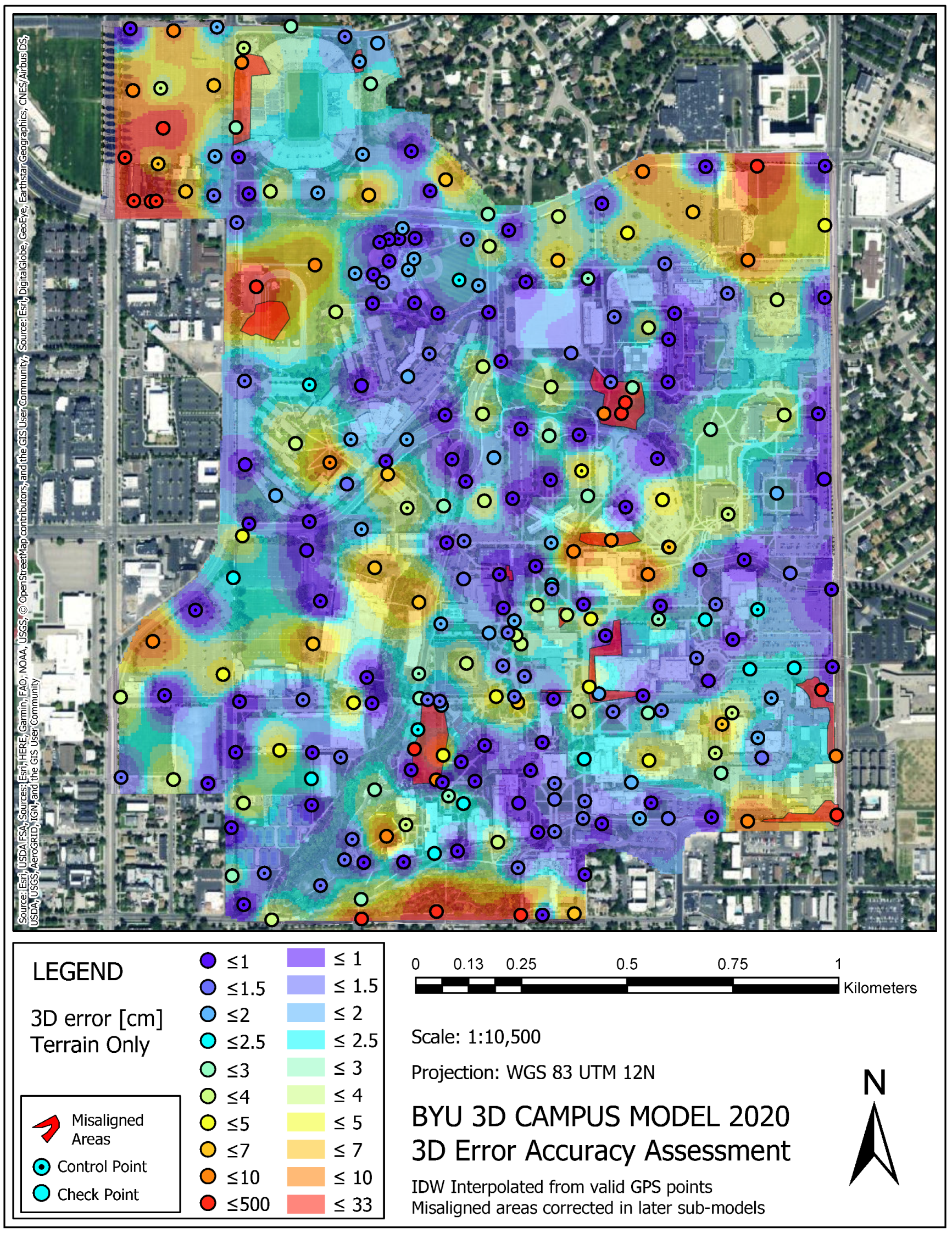
4.2.1. Absolute Accuracy Assessment

After the model was reconstructed (one year after data collection began) GPS points were again taken around campus but this time to use as CPs. Points were planned before collection and were taken as far between control points as possible. These points likely represent the areas with the highest error on campus due to their furthest distance from ground control. A total of 116 CPs were collected and subsequently added to ContextCapture and tagged.
Model error as a whole was measured by summing the positive and negative errors in the X, Y, and Z directions. Table 3 shows that the full model mean error for each direction remained under 0.55 cm with a confidence interval that contains 0. This result assures that the whole model is likely within a couple centimeters of BYU campus’ exact location on Earth.
Average model error was calculated using weighted means to account for unequal sample sizes between GCPs and CPs. It was assumed that GCPs and CPs constituted the areas of campus with the best and worst error measurements and that equally weighing and taking the average for each provides analogous error to what one would have obtains when randomly sampling a point. The results from this analysis are detailed in Table 4. The average error was 3.3 cm with a 95 % confidence interval ranging from 2.7 3.9 cm. The standard deviation for this average was 3.4 cm. Root mean squared (RMS) reprojection error in pixels was 1.6 and had a 95 % confidence interval of 1.4 1.8 px. Standard deviation for RMS of the reprojection error was 1.2 px. When looking at GCPs and CPs individually, CPs assumed to represent the “worst” locations in the model had an average 3D error of 4.6 cm while GCPs have an average 3D error of 1.5 cm.
This model can not only be used for visual aesthetics, but may be used for design and accurate historical preservation or reconstruction. Areas that contain misalignments (12 areas total) as seen in Figure 15 must be considered and new updated versions of these areas were made that have similar accuracy to the rest of campus. Changes to campus over the past year (2020–2021) since the model data were collected can be a limiting factor in potential applications and requires consideration.
Because campus resolution and accuracy vary depending on each region, an interpolated inverse distance weighted error map was created in Esri’s ArcGIS Pro software to provide another reference for model accuracy that accounted error variability due to campus location (see Figure 15) [56]. This map provides more data for model users since model accuracy varies and in many applications, only a small region of campus is being observed or used.
Data for this absolute error analysis were collected on flat ground and does not account directly for vertical features or vegetated areas of the model. As in all photogrammetry models, skinny objects such as lamp poles, branches, wires, railings, and so on, often fail to model accurately. Glass, water, or other reflective surfaces frequently possess holes or create non-existent modeled surfaces. Some of these errors were edited manually after the model was run, but it was not timely or feasible to edit every region of campus. Floating objects such as tree or bush limbs or lamps were left in the model in order to help planners or future users of the model to be able to see where objects were, even if the noted objects did not model to complete accuracy. Moving or detailed objects, such as vehicles and vegetation, can also model poorly because photogrammetry and SfM methods assume that objects remain stationary during data capture. This accuracy analysis does not account for these small scale errors and limitations and must be considered before model use.
In an effort to quantify relative error and determine local uses for the model, another accuracy analysis (relative accuracy) was conducted via tape measure and SLAM LIDAR.

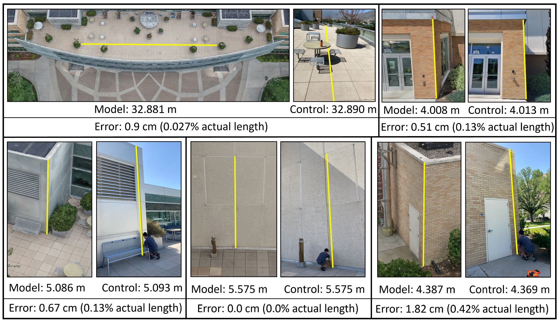
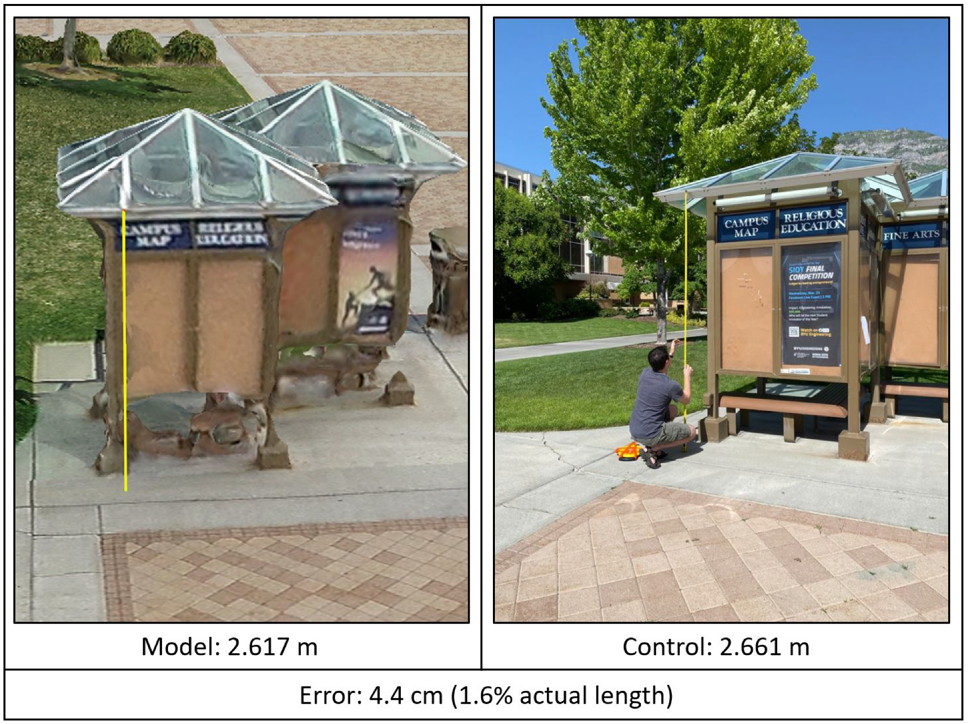
4.2.2. Relative Accuracy

At nearly the same time that CPs were collected, multiple physical measurements were also collected around campus to analyze relative accuracy. A focus was placed on measuring vertical and non-ground level surfaces since the absolute GPS CPs’ accuracy assessment was based largely on flat level ground surfaces. Some of these measurements and the their resulting errors can be seen in Figure 16. The absolute value average measured error was 0.64 cm or 0.16% of the actual tape measure length, which is well within range of human surveying error. The lower and upper 95 % bounds for these values were 0.25 cm and 1.03 cm, and 0.06 % and 0.26 % , respectively, with standard deviations of 0.65 cm and 0.17 % . Three of the twelve measurements had no error down to the millimeter. These measurements that had no error were included in the average by adding 0.4 mm error or 0.004 % because these numbers represent a conservative estimate of actual error by using the next significant figure below what was able to be measured. Based on these findings, it appears that vertical relative error in the model is not notably different than horizontal error. Areas with poor GSD on surfaces and overhangs were not included in this sampling and can be expected to have higher error, but such error is often readily identifiable as seen in Figure 17 because the textured mesh warps around what should be sharp corners.

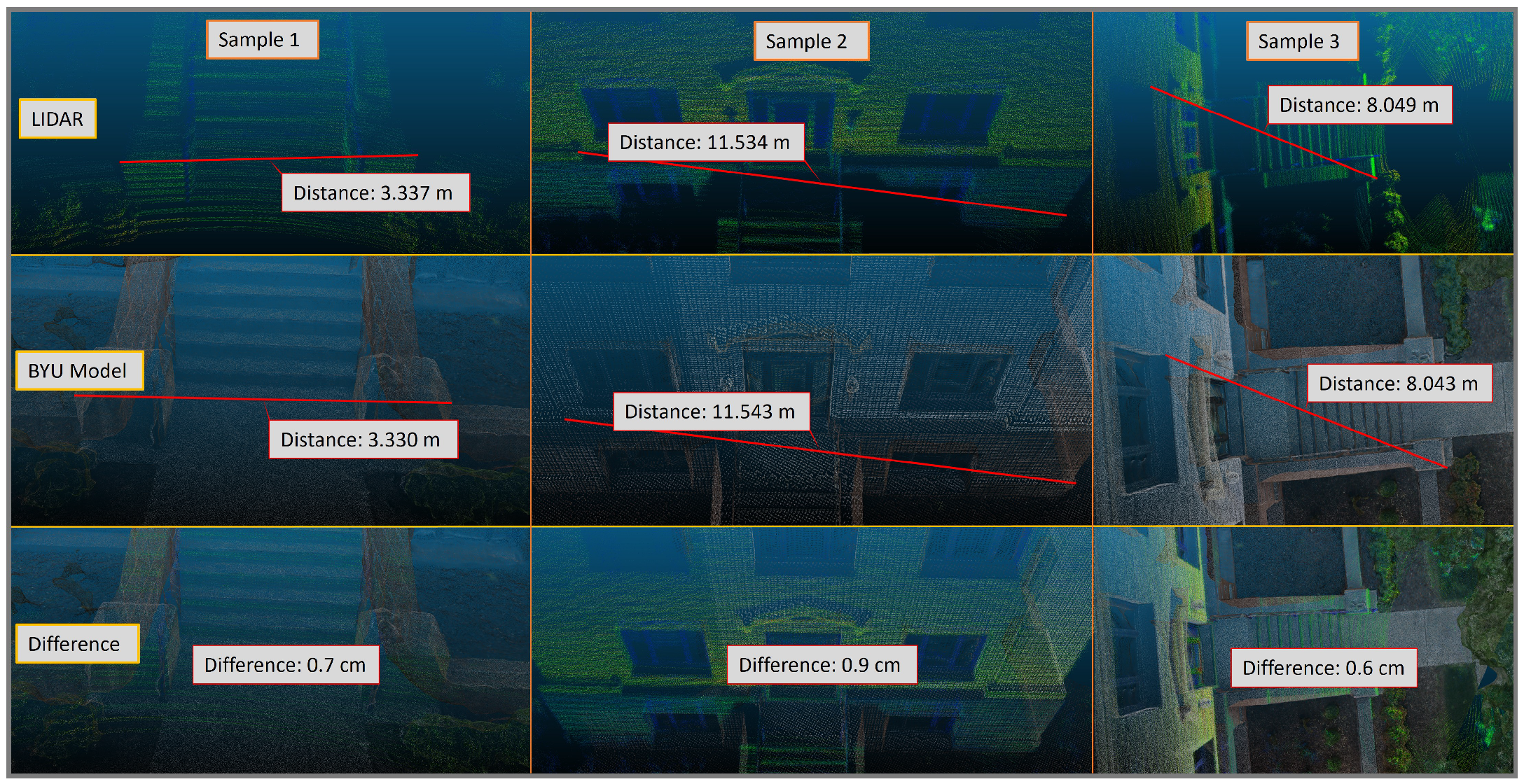
4.2.3. SLAM-Based LIDAR Comparison

While the LIDAR point clouds generated from the Velodyne VLP-16 sensor are not accurate to survey standards; accuracy for this particular sensor is reported to be around 3 cm [89]. Raw LIDAR data were processed using the Kaarta Cloud via simultaneous localization and mapping (SLAM) technology [81]. While a complete comparison of the BYU model and a LIDAR model of campus is not possible due to the few sample LIDAR surveys taken at the time of the model, three comparisons were conducted between BYU model segments and their counterpart LIDAR scans for additional relative accuracy analysis.
The Velodyne VLP-16 sensor configuration used for our scans did have GPS data, thus making direct cloud to cloud comparisons difficult and subject to software alignment error. to avoid such error, direct point to point distance measurements were made on the point clouds themselves for comparison as seen in Figure 18. Three comparison distances were selected from each of the three model comparisons totaling nine sample measurements. The total average difference between models was 0.68 cm or 0.1% of the LIDAR measured lengths.
These measurements add to the relative accuracy tape measure analysis’s assurance that the model is within centimeter accuracy when comparing distances between local objects or points (up to 33 m). Both relative accuracy assessments provided measurement differences ranging from only 0.64–0.68 cm or 0.16–0.10% of the control length. Both of these analysis suggest that local model measurements can be made within cm accuracy for similar resolution and coverage areas of the model.

4.3. Optimized Flight Path Model Results

Two areas of campus were imaged using BYU ROAM’s optimized a priori algorithm and app Volare. While only the data from one of these areas were used in the final model, this section addresses the possible benefits for this type of data collection in historical preservation and 3D modeling.

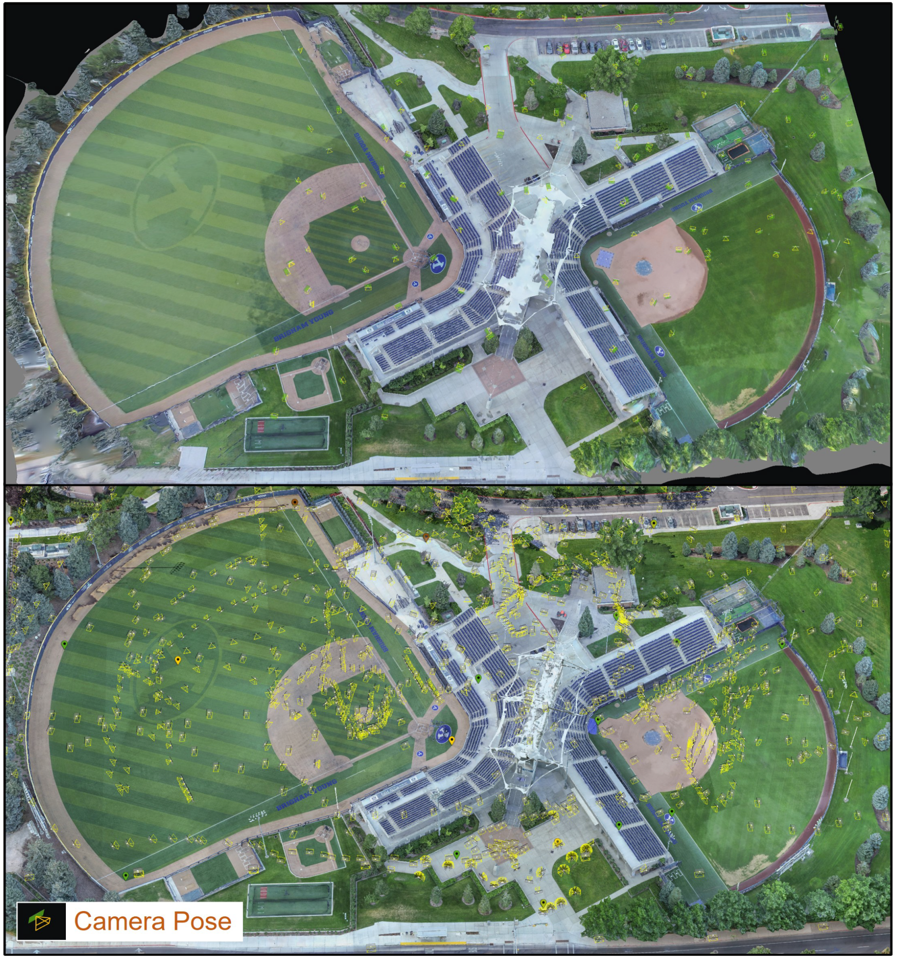
4.3.1. Miller Baseball and Softball Park Optimized Flight Model

Miller Park was imaged with both optimized (see Section 2.3.2) and manual drone and terrestrial imaging methods for the final model. Another model using only the optimized flights was made and both models can be compared in Figure 19. For both optimized and manual data sets, the park was imaged in the morning hours before the sun rose above the mountains in order to avoid shadows, and were imaged in two sequential days. Typically, this is not a recognized and generally accepted best practice in SfM modeling, but due to minimal changes and no events between the two days, the combined model meshed nearly seamlessly with the exception of the canopy cover in both models (the canopy cover did not model well due to low light and little change in color or detail throughout the whole material for key points to be formed as generally known in photogrammetry).
The optimized model used 152 photos (of the 153 taken) in the aerotriangulation and 8 GCPs and 5 CPs. Average GSD was reported as 1.875 cm/px though some of the included pixels were from oblique images and represented areas outside of the model region such as mountains and distant structures. The alignment used a median of 25,089 key-points per photo and contained a total of 9087 tie points with a median of 229 aberration points per photo.
All optimized model GCPs and CPs averaged 3.44 cm, and a weighted error using the GCPs with CPs of 2.8 cm. These results reasonably compare to the model as a whole, which averaged a combined accuracy of 3.3 cm (also using both GCPs and CPs).
The full model used all optimized and manual photos. The optimized model, on the other hand, used only 10 % of the photos and took under 5 min to process and produces a model that qualitatively covers the area of interest with overall high quality (though the area of interest for the optimized model only included the seating structure). Further optimized flights based off this model in an iterative process could continue to give greater GSD and accuracy while economizing data storage and time. Using this case study’s campus (or most current) model for a base to plan additional flights would streamline the next campus modeling project’s efficiency.

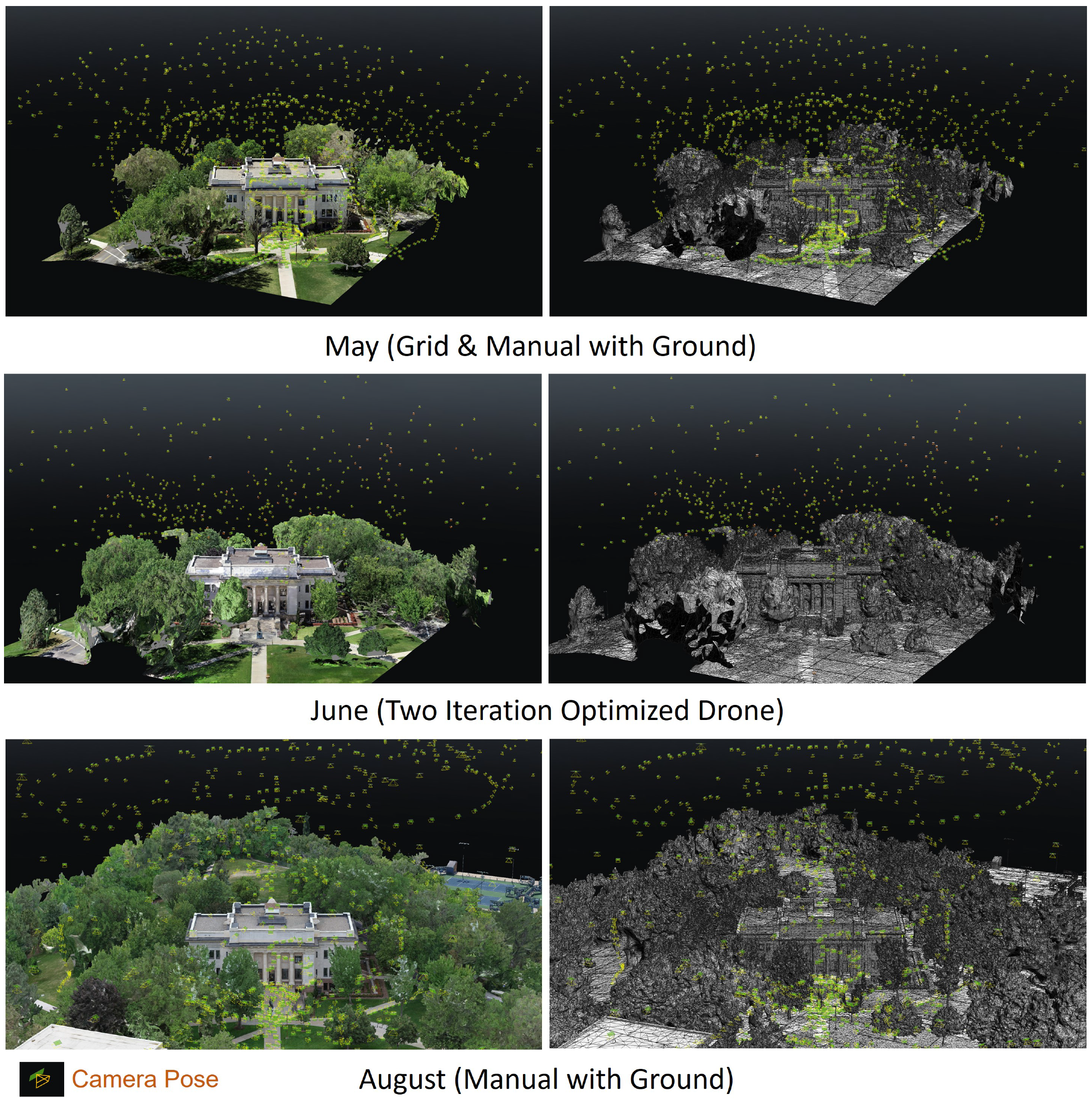
4.3.2. Karl G. Maeser Building Optimized Flight Model

Data for the historical MRSB were gathered on three individual occasions with only the last making it into the final model. The first and last models were conducted the same way as the rest of campus with ground images, and dynamic manual flights (with the first also using automated grid flights). The second set of flights were conducted using optimized flight paths (see Section 2.3.2); however, the final mission included cloudy weather and photogrammetrically conducive lighting that merited inclusion in final model reconstruction). Comparisons of data and model differences appear in Figure 20 and Table 5.
The optimized photos were also taken via a different camera than were the May and August manual models (Camera Model FC6310 via a DJI phantom 4 Pro instead of the Zenmuse X4S on an Inspire 2) due to safety precautions. The difference in photo resolution and quality constitute a confounding variable that makes in depth comparisons between models and data aquisition methods difficult; however, basic comparisons of the resulting models for the purpose of this study and proposing future research is still of value and mentioned briefly in this section.
The optimized model shown in the center of Figure 20 was recreated using all the photos taken in a two-step iteration process. The first flight was taken with a distance from the imaging target of 150 ft and was based off of the May model while the second flight was taken with a 75 ft distance and based off of the 150 ft flight model. Table 5 show results including an alignment using all photos, and one including only the last 75 ft photos (which by design are all that is needed in recreating the final model of an iterative process).
When comparing both manual data acquisition models with the optimized model, both manual models had higher GSDs in part because ground photos were not included in the optimized model, which affects the resolution as the higher megapixel count and shorter average imaging distances of the ground photos greatly reduce overall GSD. However, the fewer number of photo required for processing (<25%–<40% depending on wither one or two iterations are considered) and the cut in model processing time (at least by 85 % for last iteration photo model) is significant. Alignment success with manual and grid flights, and ground photos for the May and August models were unusually high compared to most other areas of campus (Around 78 % success as noted in Table 2). In general, BYU ROAM’s optimized flight planning shows potential to reduce the number of unnecessary photos taken in an oblique detail based model and may also increase alignment success.
If further model additions/updates or future campus models of BYU are desired, optimized flight paths may be an efficient step-out method of to acquire and generate large-scale models, especially since most areas now have a preliminary model as a basis for optimized flights. Even a highly experienced photogrammetry pilot will take photos that are not needed or miss significant details. Supplementary ground photos would still compliment optimized data if ties between the optimized flights and the ground can be made in the model generating software. Supplementary manual add-on photos may still be needed to "close the gap" in some optimized and ground photo survey situations where flying too low to the ground creates unacceptable safety risk (quantitative generalization of these assertions from observation is outside the scope of this work).

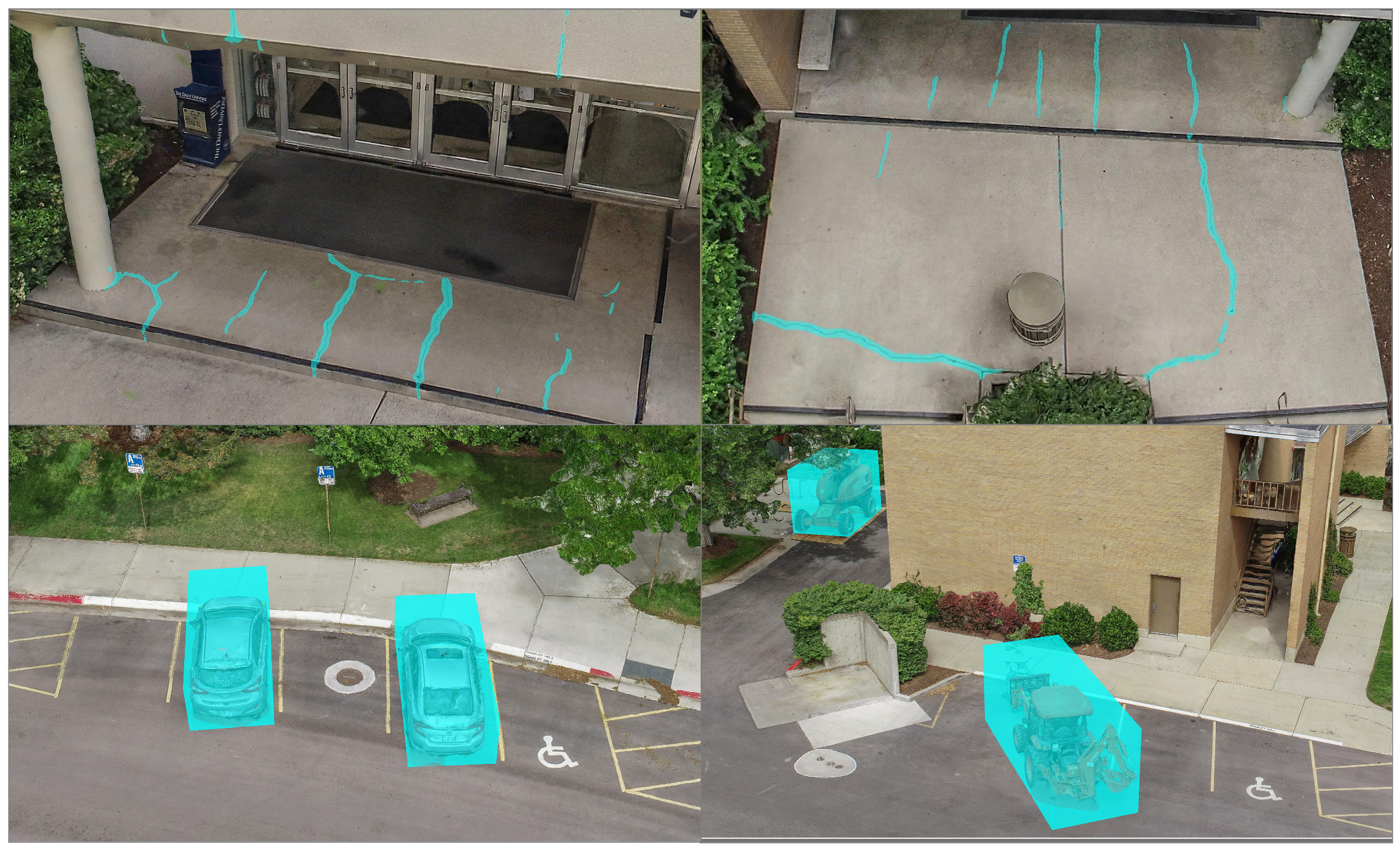
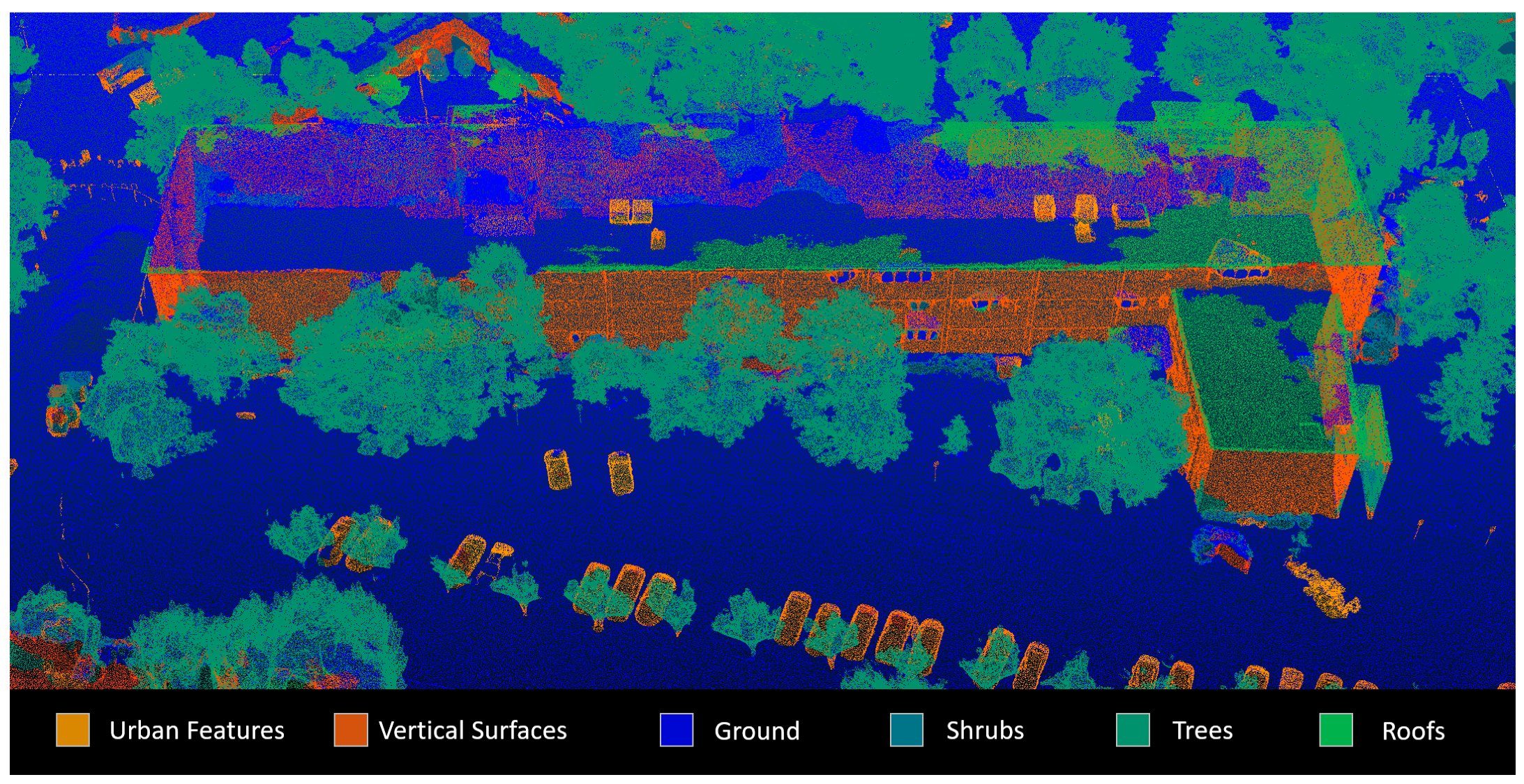
4.4. Machine Learning and Object Recognition of Final Model

ContextCapture includes in-program machine learning capabilities, such as object recognition and automated annotations, that were applied to the BYU campus model in this case study. Recognition of cracks and vehicles were run as an experiment and shown in Figure 21. Due to the sub-centimeter accuracy of the model, the computer successfully identifies and highlights the major cracks and flaws in the concrete, though breaks in concrete blocks/human-made cracks were often identified.
Point cloud segmentation samples were ran that separated features such as vertical surfaces, shrubs, trees, roofs, and ground (see Figure 22). This method of segmentation machine learning can be very useful in identifying object areas for campus studies such as trees or vegetation.
In order to do object recognition for other features, the software only needs a provided data set of pictures to learn from—i.e., several hundred pictures of manholes or other features could serve as a training data set, and then the software could highlight and/or count all of the manholes or other desired features on campus. The training data set could come from photos on the BYU campus or from other sources. The plethora of other objects and features that could leverage the 3D model of the university’s campus are left as a point for future development and application, but could include various objects and features of interest (statues, building wear, water damages, etc.). Other aspects of applying machine learning, such as auto-alignment and unsupervised machine learning that could be applied to this case are out of the scope of this study.

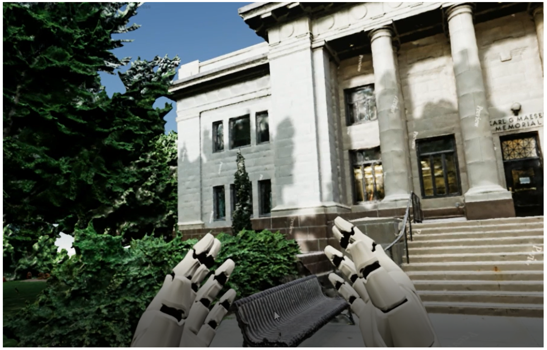
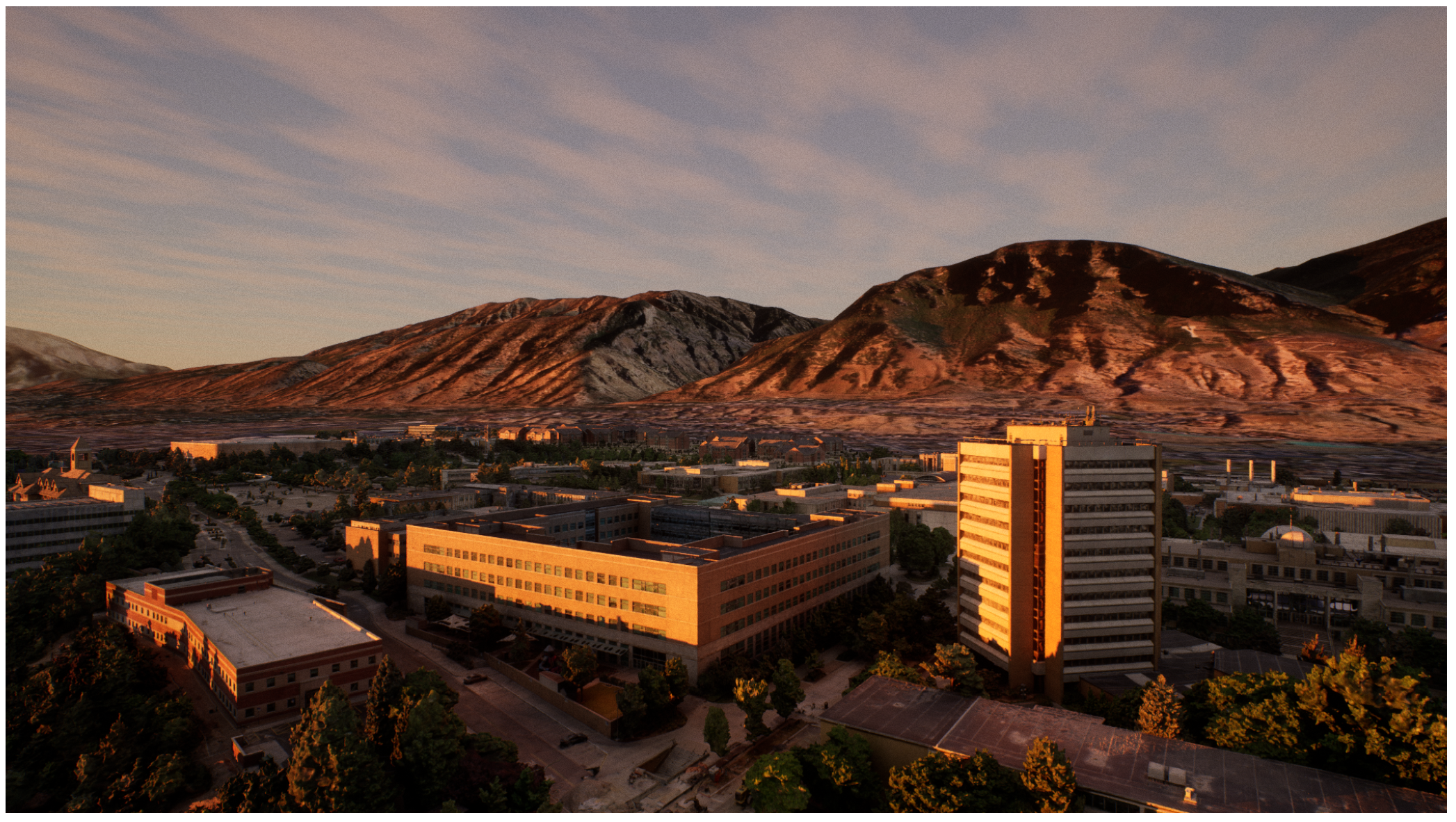
4.5. Augmented and Virtual Reality and Realistic Visualization
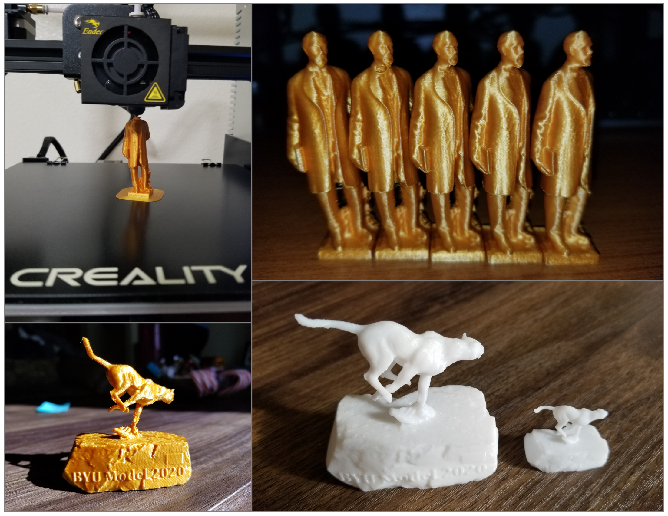
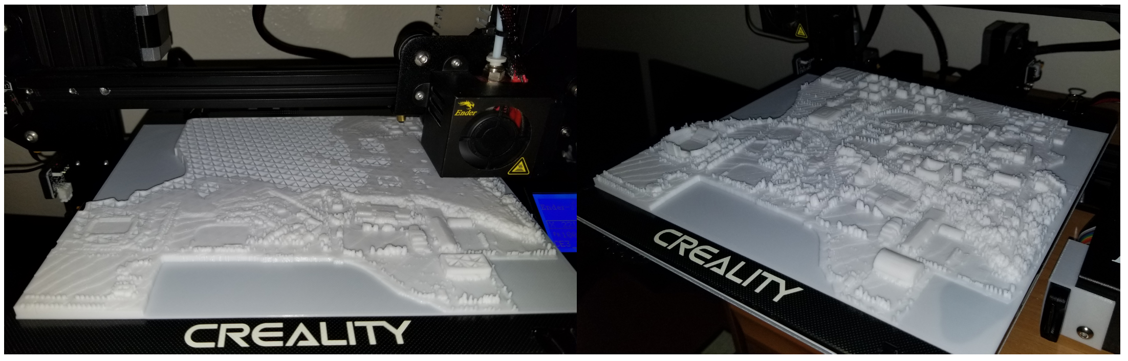
Although an in depth study the BYU model in VR format is not a focus of this case study nor paper, some rudimentary work to make sections of the model function in a VR environment was conducted by BYU’s Mixed Reality Lab (see Figure 23). FBX and OBJ files were imported into Unreal Engine 4 where lighting and other color options are adjustable for the user experience [90]. An Oculus Quest 2 [91] linked to a VR ready computer was used for testing. It is of note that the current OBJ and FBX export’s textures are not of the same detail and quality as is the 3MX format used for the online viewing application or cinematic videos. Further work incorporating more detail into the models continues.
We rendered 360° video renderings of the model that are able to be viewed in VR on YouTube that give an immersive experience to viewers (see Figure 24). These videos do not allow the user to move in 3D space but do keep the original 3MX textures (via 3SM format) and are rendered in 8K for 360°. Because all 8k pixels are distributed in 360°, the model in this format does not show as much detail as in the online viewing app, but is sufficient for simple demonstration purposes.
New technology using an early access version of Unreal Engine 5 also show promise in enabling larger data visualization for lifelike model renderings and VR adaptation. Figure 25 shows an FBX export of the model in a new software for a special interactive display project on BYU campus [90].
AR and VR are both applications that could be used for campus tours or even planning and development. Additional data such as proposed CAD models of new structures, or realistic vegetation additions to proposed green space could be imported for immersive visualization and educated decision-making.

4.6. 3D Printing

3D printing and physical miniatures of parts or all of BYU campus represent another area of interest and possible use for the BYU digital 3D model. All modeled areas of campus were also exported into STL file format (ideal for 3D printing). Some elementary printing work was conducted using a cheap consumer grade Ender 3 printer from Creality in a plain white and gold metallic filament. Areas such as statues that were captured in high detail are optimal objects for 3D prints as seen in Figure 26, though entire buildings or regions of campus can be printed but require separate model block merging due to the BYU model being divided into 2063 parts.
Model smoothing was required and additional edits or add-ons such as trimming or model embroidering were conducted in version 18.0.1931.0 of a free Microsoft app called 3D Builder [92]. Areas on campus with vegetation or floating objects in the model would require additional clean up before 3D printing, but the base model provides a framework that can be a foundation for more efficient and streamlined use.
One possible workaround to printing small versions of the entirety of BYU Campus was conducted by 3D printing based off a campus digital elevation map (DEMa) which is shown in Figure 27. In this case, model under hangs and other covered features were not taken into account and the DEMa used represented only the highest elevations from an aerial view. Larger models with such features can be created but would require more pre-possessing and have not yet been executed.

5. Discussion and Analysis

The 1.65 trillion-pixel model of BYU’s 1 . 7 2 km campus captures the entire campus during the moments of the historic COVID-19 Pandemic. While significance exists for practical applications beyond heritage and preservation (maintenance, public relations, development planning, smart campus, etc.), the large-scale 3D model digitizes and preserves the history of over 75 significant buildings. Among these 75 buildings include newly constructed edifices such as the West View, Life Science and the Engineering buildings, and renders older historic buildings such as the MSRB at centimeter level accuracy and precision. The growth of additional technologies such as AR and VR present opportunities for the large-scale model to allow future students and interested parties to digitally see and visit exactly what the BYU campus was like during the COVID-19 Pandemic. Not only does the model capture a historic time, the model also demonstrates that given enough photos and processing power, UAV photogrammetry can realistically model large swathes of complex structures and land.
From inception, BYU seeks to better serve an ever-growing student body. This includes the renovation and expansion of campus buildings to meet the demands of each new decade as demonstrated by the refurbishment of older structures such as the MSRB and the construction of new buildings such as the School of Music. This model preserves BYU’s changing campus at a critical moment in history, maintaining a highly detailed image of the buildings and grounds that can be researched and enjoyed for many decades to come.
Use of supervised machine learning to run object recognition through ContextCapture highlights how algorithmic solutions to age-old problems are now accessible to industry and academia without the need for underlying detailed domain knowledge to apply algorithmic solutions. Identifying concrete cracks and vehicles serves as a beginning to what could lead to more modern and informed maintenance and construction projects.
The large scale and high detail of the model makes this study significant. In previous works by the authors and others, the number of pixels (or points) numbered in the millions to billions [25,38,42,53,75,93]. In this case study a much larger 1.65 trillion-pixel 3D model was successfully made. Care towards the edges of the 31 model segments with regard to lighting, GCPs, and alignment stitched the complete model together without noticeable boundaries. The data processing required over 2 months despite leveraging 4–5 computers in a cluster using 16 GB of RAM per tile for 2063 tiles. When considering relative accuracy, the model presents accuracies between 0.25 cm and 1.03 cm in the region of 95 % that excludes the upper and lower absolute bounds. In other words, the model delivers consistent sub-centimeter accuracy for essentially the entire 1 . 7 2 km of the BYU campus with a standard deviation of 0.65 cm.
Potential cost-benefits exist for using photogrammetry and SfM modeling in similar modeling situations to BYU campus as an alternative to LIDAR. While LIDAR has become an accepted standard for 3D modeling accuracy and detail, the cost of equipment between the two methods can vary drastically. The entire equipment set used for this photogrammetry project would average a cost of about $24,000 in 2021 with the GPS receiver unit accounting for half that cost. A similar LIDAR setup with separate drone and terrestrial units might begin around $95,000. In other words, photogrammetry modeling equipment for large scale areas (excluding software costs) would likely at least require a quarter of the equipment budget as a LIDAR equivalent solution though price estimates and equipment choices vary greatly. LIDAR however, would likely save on data acquisition and processing time and costs which could make up a decent portion of the price difference depending on the project and SfM data acquisition efficiency. Thus, when optimized or efficient photogrammetry modeling can be conducted, SfM UAV and terrestrial photo based modeling may be an attractive economic modeling workflow for large and complex sites. True RTK drones could reduce data acquisition time and cost by eliminating the need for GCP surveying and would further make photogrammetry modeling a more efficient solution in some situations [94,95,96].

6. Conclusions and Future Work

This case study contributes to existing research related to UAVs and SfM in various ways. The sheer extent and scope of the project and study are novel and provide a detailed description of a viable workflow and best practices for efficient photogrammetry data collection and large scale processing. This includes the uncommon beneficial practice of incorporating both terrestrial and UAV based photo data into models of the same area. Machine learning and optimization of UAV photo collection using automated flight planning algorithms also adds new value and potential to large scale modeling and especially the idea of repeated update modeling. Exploration into viable use-cases for historical and photogrammetry modeling are also researched and explored adding viable ideas and proof of concept results that can be applied to other modeling projects and studies of this kind. The absolute and relative accuracies analyzed in this case study also demonstrate that UAV photogrammetry can be used for purposes such as improving maintenance or assisting in construction planning projects. In addition to this case study’s academic contributions, the resulting campus 3D model contributes to the historical heritage preservation of the university and represents a unique snapshot in history that can be used in innumerable ways for perpetuity. The final model uses 80 , 384 photos and is arguably one of the largest and most detailed single photogrammetric 3D models developed by SfM to date.
It is significant for BYU’s history that over 75 buildings are digitally preserved to sub-centimeter resolution in the final model. The fact that the 3D model-scape is from the COVID-19 pandemic (between April and August 2020) ensures that the model is from a key point of interest in history similar to other major world events such as World War I and the 1918 influenza pandemic.
Step out deployment beyond the detailed scale-up in this paper could include different views from technology such as infrared cameras, 360° cameras, and LiDAR incorporated into the model. Auto-updated mapping of normal and infrared views could give insights into greener sustainability, 360° cameras might be able to save on data acquisition time or even model inside of structures, and LiDAR would be ideal for indoor scans and for comparison to original model work. The model provides a platform for further AR and VR applications, which would add nuance to UAV photogrammetric technology and applications.
Accuracy comparisons between modeling methods (such as varying the number of control points or flight path differences) using CloudCompare with accompanying quantitative and qualitative analysis is left to future studies. Aspects of machine learning algorithms such as unsupervised machine learning and an NBV approach on the massive scale viz Arce et al. [42] are a step beyond current practices. Besides the combination of the detailed scaled-up model and the algorithmic techniques throughout the process, more exploration work remains. Future work could include VR level of detail (LOD) tours and simulations, automated updates to the model, potential urban planning for sustainability purposes, large 3D printing projects, and a smart college campus.
In the event of hazard reconnaissance, this work also provides a base model for change detection, study, and monitoring after traumatic or damaging events such as earthquakes such as that seen in Freeman et al. [47] (earthquakes being of particular concern to BYU and the surrounding region as a whole). Structural damage as well as mass movement can be measured and compared in such situations and is an area of study rarely conducted due to limited before-and-after models for most hazard locations.

Author Contributions

B.E.B., as first author, conducted the large-scale BYU case study and led the fieldwork, acquisition of data, processing of data, and interpretation of results. C.A.V. complimented the literature review, explained the algorithms, interpreted results, and assisted editing. Historical research and applicability to heritage and historical preservation was led by H.B. who also assisted in data acquisition and processing. M.P. assisted in photo editing and model post-processing and writing the literature review on UAV and modeling history. K.M. helped compile and synthesis data for this paper and helped with post-processing model efforts. K.W.F. leads the Research in Optimized Aerial Modeling (ROAM) research group and lent UAV modeling expertise and project guidance. J.D.H. leads the Process Research and Intelligent Systems Modeling (PRISM) research group and vetted the references to automation, algorithms, and machine learning. All authors have read and agreed to the published version of the manuscript.

Funding

This research was funded by BYU University Communications and the BYU Ira A. Fulton College of Engineering. Research used in this project from BYU ROAM was funded by the Center for Unmanned Aircraft Systems (C-UAS), a National Science Foundation Industry/University Cooperative Research Center (I/UCRC) under NSF Award No. IIP-1650547 along with significant contributions from C-UAS industry members.

Institutional Review Board Statement

Not applicable.

Informed Consent Statement

Not applicable.

Data Availability Statement

An online version of the BYU model for public viewing and updated information can be found at https://3dbyu.byu.edu (accessed 6 November 2021). Additional data presented in this study may be available on request from the corresponding author.

Acknowledgments

The authors would like to acknowledge the assistance of Ben Horne, Sarah McClellan, Elodie Ence, Nicole Hastings, Matthew Gabbitas, Joseph Janson, Jared Fuerst, Brigitte Berrett, Adam Foulk, Izaak Cooper, and Michael Freeman for their help with data acquisition field work. Anna Cardall, Madison Palmer, Lily Mae Rich, Mohamad Chebli, Blair Hanson, Heather Siddoway, and Kaleb Markert for their help with photo reprocessing, model post-processing and edits, and GPS accuracy assessment surveying. Joshua Hammond, Zack Mortensen, for their help with optimized flight planning. Michael Crookston at BYU for his support with model hosting. Craig Harris for his work getting the BYU Model into VR. ZiRui Su for help with model uses and paper research. David Wingate and Vin Howe for Unreal Engine visualization. The authors further acknowledge BYU University Communications and specifically Julie Walker, Brian Wilcox, and Matt Mitchell for their help sharing this project and research.

Conflicts of Interest

The authors declare no conflict of interest. The funders provided feedback on industrial relevance of the study and directed the research focus towards multi-scale monitoring. The funders were not involved in the study design or analysis.

References

  1. Wilkinson, E.L.; Skousen, W.C. Brigham Young University: A School of Destiny; Brigham Young University Press: Provo, UT, USA, 1976. [Google Scholar]
  2. Deseret News. 9 Important Events in BYU History. 2015. Available online: https://www.deseret.com/2015/10/15/20765089/byu-history-9-important-events (accessed on 6 November 2021).
  3. Building Inventory Brigham Young University October 2019. 2019. Available online: https://brightspotcdn.byu.edu/03/90/ba644d56416db62461d1e29777d3/building-inventory.pdf (accessed on 6 November 2021).
  4. Brigham Young University News Bureau. Maeser Memorial Building, ca. 1911, Courtesy, Perry Special Collections; Harold B. Lee Library, Brigham Young University: Provo, UT, USA, 2005. [Google Scholar]
  5. Winters, C.R. How Firm a Foundation. 2012. Available online: https://magazine.byu.edu/article/how-firm-a-foundation/ (accessed on 6 November 2021).
  6. Daines, G. The City Beautiful Movement and the Karl G. Maeser Building. 2012. Available online: https://scblog.lib.byu.edu/2012/09/05/the-city-beautiful-movement-and-the-karl-g-maeser-building/ (accessed on 6 November 2021).
  7. Gardener, P.B. 3186 Windows into Engineering. 2019. Available online: https://magazine.byu.edu/article/3186-windows-into-engineering/ (accessed on 6 November 2021).
  8. Hollingshead, T. BYU Announces Construction of New West View Building. 2018. Available online: https://news.byu.edu/news/byu-announces-construction-new-west-view-building (accessed on 6 November 2021).
  9. Hollingshead, T. BYU Announces Approval to Construct New Music Building. 20 February 2020. Available online: https://news.byu.edu/announcements/byu-announces-approval-to-construct-new-music-building (accessed on 6 November 2021).
  10. Walker, M.R. BYU, Still: Covid-19 and Its Impact. 2020. Available online: https://magazine.byu.edu/article/coronavirus-covid-19/ (accessed on 6 November 2021).
  11. Cummings, A.R.; McKee, A.; Kulkarni, K.; Markandey, N. The rise of UAVs. Photogramm. Eng. Remote Sens. 2017, 83, 317–325. [Google Scholar] [CrossRef]
  12. Rathje, E.M.; Franke, K.W. Remote Sensing for Geotechnical Earthquake Reconnaissance. Soil Dyn. Earthq. Eng. 2016, 91, 304–316. [Google Scholar] [CrossRef] [Green Version]
  13. Schenk, T. Introduction to Photogrammetry; The Ohio State University: Columbus, OH, USA, 2005; Volume 106. [Google Scholar]
  14. Ullman, S. The interpretation of structure from motion. Proc. R. Soc. Lond. Ser. B Biol. Sci. 1979, 203, 405–426. [Google Scholar]
  15. Faugeras, O.D.; Lustman, F. Motion and structure from motion in a piecewise planar environment. Int. J. Pattern Recognit. Artif. Intell. 1988, 2, 485–508. [Google Scholar] [CrossRef] [Green Version]
  16. Bolles, R.C.; Baker, H.H.; Marimont, D.H. Epipolar-plane image analysis: An approach to determining structure from motion. Int. J. Comput. Vis. 1987, 1, 7–55. [Google Scholar] [CrossRef]
  17. Koenderink, J.J.; Van Doorn, A.J. Affine structure from motion. JOSA A 1991, 8, 377–385. [Google Scholar] [CrossRef] [PubMed]
  18. Sturm, P.; Triggs, B. A Factorization Based Algorithm for Multi-Image Projective Structure and Motion. 1996, pp. 709–720. Available online: https://bit.ly/3qLzgHK (accessed on 6 November 2021).
  19. Bartoli, A.; Sturm, P. Structure-from-motion using lines: Representation, triangulation, and bundle adjustment. Comput. Vis. Image Underst. 2005, 100, 416–441. [Google Scholar] [CrossRef] [Green Version]
  20. Brostow, G.J.; Shotton, J.; Fauqueur, J.; Cipolla, R. Segmentation and Recognition Using Structure from Motion Point Clouds. 2008, pp. 44–57. Available online: https://bit.ly/2YSVb42 (accessed on 6 November 2021).
  21. Westoby, M.J.; Brasington, J.; Glasser, N.F.; Hambrey, M.J.; Reynolds, J.M. ‘Structure-from-Motion’photogrammetry: A low-cost, effective tool for geoscience applications. Geomorphology 2012, 179, 300–314. [Google Scholar] [CrossRef] [Green Version]
  22. Fonstad, M.A.; Dietrich, J.T.; Courville, B.C.; Jensen, J.L.; Carbonneau, P.E. Topographic structure from motion: A new development in photogrammetric measurement. Earth Surf. Process. Landforms 2013, 38, 421–430. [Google Scholar] [CrossRef] [Green Version]
  23. Franke, K.W.; Zimmaro, P.; Lingwall, B.N.; Kayen, R.E.; Tommasi, P.; Chiabrando, F.; Santo, A. A Phased Reconnaissance Approach to Documenting Landslides Following the 2016 Central Italy Earthquakes. Earthq. Spectra 2018, 34, 1693–1719. [Google Scholar] [CrossRef]
  24. Wu, C. Towards Linear-Time Incremental Structure from Motion. 2013, pp. 127–134. Available online: https://bit.ly/3cjXKzf (accessed on 6 November 2021).
  25. Palmer, L.M.; Franke, K.W.; Abraham Martin, R.; Sines, B.E.; Rollins, K.M.; Hedengren, J.D. Application and Accuracy of Structure from Motion Computer Vision Models with Full-Scale Geotechnical Field Tests. 2015, pp. 2432–2441. Available online: https://bit.ly/3CnDEib (accessed on 6 November 2021).
  26. Ahad, M.A.; Paiva, S.; Tripathi, G.; Feroz, N. Enabling technologies and sustainable smart cities. Sustain. Cities Soc. 2020, 61, 102301. [Google Scholar] [CrossRef]
  27. Abujubbeh, M.; Al-Turjman, F.; Fahrioglu, M. Software-defined wireless sensor networks in smart grids: An overview. Sustain. Cities Soc. 2019, 51, 101754. [Google Scholar] [CrossRef]
  28. Alrashed, S. Key performance indicators for Smart Campus and Microgrid. Sustain. Cities Soc. 2020, 60, 102264. [Google Scholar] [CrossRef]
  29. Boursianis, A.D.; Papadopoulou, M.S.; Diamantoulakis, P.; Liopa-Tsakalidi, A.; Barouchas, P.; Salahas, G.; Karagiannidis, G.; Wan, S.; Goudos, S.K. Internet of Things (IoT) and Agricultural Unmanned Aerial Vehicles (UAVs) in smart farming: A comprehensive review. Internet Things 2020, 100187. [Google Scholar] [CrossRef]
  30. Arifitama, B.; Hanan, G.; Rofiqi, M.H. Mobile Augmented Reality for Campus Visualization Using Markerless Tracking in an Indonesian Private University. Int. J. Interact. Mob. Technol. 2021, 15, 21–33. [Google Scholar] [CrossRef]
  31. Pavlik, A. Offer virtual reality tours to attract prospects who can’t make it to campus. Enroll. Manag. Rep. 2020, 24, 6–7. [Google Scholar] [CrossRef]
  32. Wu, B.; Wang, Y.; Liu, R.; Tan, S.; Hao, R. Research of Intelligent Campus Design Based on Immersive BIM + VR Technology. J. Phys. Conf. Ser. 2021, 1885, 052053. [Google Scholar] [CrossRef]
  33. Franke, K.W.; Rollins, K.M.; Ledezma, C.; Hedengren, J.D.; Wolfe, D.; Ruggles, S.; Bender, C.; Reimschiissel, B. Reconnaissance of Two Liquefaction Sites Using Small Unmanned Aerial Vehicles and Structure from Motion Computer Vision Following the April 1, 2014 Chile Earthquake. J. Geotech. Geoenviron. Eng. 2017, 143, 11. [Google Scholar] [CrossRef]
  34. Ruggles, S.; Clark, J.; Franke, K.W.; Wolfe, D.; Hedengren, J.D.; Martin, R.A.; Reimschiissel, B. Comparison of SfM Computer Vision Point Clouds of a Landslide from Multiple Small UAV Platforms and Sensors to a TLS based Model. J. Unmanned Veh. Syst. 2016, 4, 246–265. [Google Scholar] [CrossRef]
  35. Martin, R.; Rojas, I.; Franke, K.; Hedengren, J.; Martin, R.A.; Rojas, I.; Franke, K.; Hedengren, J.D. Evolutionary View Planning for Optimized UAV Terrain Modeling in a Simulated Environment. Remote Sens. 2015, 8, 26. [Google Scholar] [CrossRef] [Green Version]
  36. Martin, R.A.; Blackburn, L.; Pulsipher, J.; Franke, K.; Hedengren, J.D. Potential benefits of combining anomaly detection with view planning for UAV infrastructure modeling. Remote Sens. 2017, 9, 434. [Google Scholar] [CrossRef] [Green Version]
  37. Bengio, Y.; Lodi, A.; Prouvost, A. Machine learning for combinatorial optimization: A methodological tour d’horizon. Eur. J. Oper. Res. 2021, 290, 405–421. [Google Scholar] [CrossRef]
  38. Hammond, J.E.; Vernon, C.A.; Okeson, T.J.; Barrett, B.J.; Arce, S.; Newell, V.; Janson, J.; Franke, K.W.; Hedengren, J.D. Survey of 8 UAV Set-Covering Algorithms for Terrain Photogrammetry. Remote Sens. 2020, 12, 2285. [Google Scholar] [CrossRef]
  39. Abrahamsen, M.; Adamaszek, A.; Miltzow, T. The art gallery problem is ∃ℝ-complete. In Proceedings of the 50th Annual ACM SIGACT Symposium on Theory of Computing, Los Angeles, CA, USA, 25–29 June 2018; pp. 65–73. [Google Scholar]
  40. Liu, J.; Sridharan, S.; Fookes, C. 6 Recent Advances in Camera Planning for Large Area Surveillance: A Comprehensive Review. ACM Comput. Surv. 2016, 49, 1–37. [Google Scholar] [CrossRef]
  41. Michael, J.B.; Voas, J. Algorithms, Algorithms, Algorithms. IEEE Ann. Hist. Comput. 2020, 53, 13–15. [Google Scholar] [CrossRef]
  42. Arce, S.; Vernon, C.A.; Hammond, J.; Newell, V.; Janson, J.; Franke, K.W.; Hedengren, J.D. Automated 3D Reconstruction Using Optimized View-Planning Algorithms for Iterative Development of Structure-from-Motion Models. Remote Sens. 2020, 12, 2169. [Google Scholar] [CrossRef]
  43. Polat, N.; Uysal, M. An investigation of tree extraction from UAV-based photogrammetric dense point cloud. Arab. J. Geosci. 2020, 13, 1–8. [Google Scholar] [CrossRef]
  44. Al-Ghamdi, J.A.; Al-Masalmeh, E.R. Heuristics and Meta-Heuristics Optimization Methods in Solving Traveling Salesman Problem TSP. Available online: https://www.ijariit.com/manuscript/heuristics-and-meta-heuristics-optimization-methods-in-solving-traveling-salesman-problem-tsp/ (accessed on 6 November 2021).
  45. Hoffman, K.L.; Padberg, M.; Rinaldi, G. Traveling salesman problem. Encycl. Oper. Res. Manag. Sci. 2013, 1, 1573–1578. [Google Scholar]
  46. Hoppe, C.; Wendel, A.; Zollmann, S.; Paar, A.; Pirker, K.; Irschara, A.; Bischof, H.; Kluckner, S. Photogrammetric Camera Network Design for Micro Aerial Vehicles; Technical Report; Institute for Computer Graphics and Vision—Graz University of Technology: Mala Nedelja, Slovenia, 2012. [Google Scholar]
  47. Freeman, M.; Vernon, C.; Berrett, B.; Hastings, N.; Derricott, J.; Pace, J.; Horne, B.; Hammond, J.; Janson, J.; Chiabrando, F.; et al. Sequential Earthquake Damage Assessment Incorporating Optimized sUAV Remote Sensing at Pescara del Tronto. Geosciences 2019, 9, 332. [Google Scholar] [CrossRef] [Green Version]
  48. Al-Betar, M.A.; Awadallah, M.A.; Faris, H.; Aljarah, I.; Hammouri, A.I. Natural selection methods for grey wolf optimizer. Expert Syst. Appl. 2018, 113, 481–498. [Google Scholar] [CrossRef]
  49. Feo, T.A.; Resende, M.G. A probabilistic heuristic for a computationally difficult set covering problem. Oper. Res. Lett. 1989, 8, 67–71. [Google Scholar] [CrossRef]
  50. Jung, D.; Dong, Y.; Frisk, E.; Krysander, M.; Biswas, G. Sensor selection for fault diagnosis in uncertain systems. Int. J. Control 2020, 93, 629–639. [Google Scholar] [CrossRef] [Green Version]
  51. Cerrone, C.; Cerulli, R.; Golden, B. Carousel greedy: A generalized greedy algorithm with applications in optimization. Comput. Oper. Res. 2017, 85, 97–112. [Google Scholar] [CrossRef]
  52. Antoine, R.; Lopez, T.; Tanguy, M.; Lissak, C.; Gailler, L.; Labazuy, P.; Fauchard, C. Geoscientists in the Sky: Unmanned Aerial Vehicles Responding to Geohazards. Surv. Geophys. 2020, 41, 1285–1321. [Google Scholar] [CrossRef]
  53. Okeson, T.J.; Barrett, B.J.; Arce, S.; Vernon, C.A.; Franke, K.W.; Hedengren, J.D. Achieving Tiered Model Quality in 3D Structure from Motion Models Using a Multi-Scale View-Planning Algorithm for Automated Targeted Inspection. Sensors 2019, 19, 2703. [Google Scholar] [CrossRef] [Green Version]
  54. Systems, B. Bentley: Advancing Infrastructure. 2020. Available online: https://www.bentley.com/en (accessed on 6 November 2021).
  55. AgiSoft Metashape Professional (Version 1.5.5). 2019. Available online: https://www.agisoft.com/ (accessed on 6 November 2021).
  56. Esri. 2021. Available online: https://www.esri.com/en-us/home (accessed on 6 November 2021).
  57. Open Source Community. CloudCompare. 2019. Available online: https://www.danielgm.net/cc/ (accessed on 6 November 2021).
  58. Klápště, P.; Fogl, M.; Barták, V.; Gdulová, K.; Urban, R.; Moudrý, V. Sensitivity analysis of parameters and contrasting performance of ground filtering algorithms with UAV photogrammetry-based and LiDAR point clouds. Int. J. Digit. Earth 2020, 13, 1672–1694. [Google Scholar] [CrossRef]
  59. Sanz-Ablanedo, E.; Chandler, J.; Rodríguez-Pérez, J.; Ordóñez, C. Accuracy of Unmanned Aerial Vehicle (UAV) and SfM Photogrammetry Survey as a Function of the Number and Location of Ground Control Points Used. Remote Sens. 2018, 10, 1606. [Google Scholar] [CrossRef] [Green Version]
  60. Jordan, M.I.; Mitchell, T.M. Machine Learning: Trends, Perspectives, and Prospects. Science 2015, 349, 255–260. [Google Scholar] [CrossRef] [PubMed]
  61. Lee, I.; Shin, Y.J. Machine learning for enterprises: Applications, algorithm selection, and challenges. Bus. Horizons 2020, 63, 157–170. [Google Scholar] [CrossRef]
  62. Scheurer, M.S.; Slager, R.J. Unsupervised machine learning and band topology. Phys. Rev. Lett. 2020, 124, 226401. [Google Scholar] [CrossRef]
  63. Davis II, R.L.; Greene, J.K.; Dou, F.; Jo, Y.K.; Chappell, T.M. A Practical Application of Unsupervised Machine Learning for Analyzing Plant Image Data Collected Using Unmanned Aircraft Systems. Agronomy 2020, 10, 633. [Google Scholar] [CrossRef]
  64. Eskandari, R.; Mahdianpari, M.; Mohammadimanesh, F.; Salehi, B.; Brisco, B.; Homayouni, S. Meta-Analysis of Unmanned Aerial Vehicle (UAV) Imagery for Agro-Environmental Monitoring Using Machine Learning and Statistical Models. Remote Sens. 2020, 12, 3511. [Google Scholar] [CrossRef]
  65. Carvajal-Ramírez, F.; Serrano, J.M.P.R.; Agüera-Vega, F.; Martínez-Carricondo, P. A comparative analysis of phytovolume estimation methods based on UAV-photogrammetry and multispectral imagery in a mediterranean forest. Remote Sens. 2019, 11, 2579. [Google Scholar] [CrossRef] [Green Version]
  66. Bolourian, N.; Hammad, A. LiDAR-equipped UAV path planning considering potential locations of defects for bridge inspection. Autom. Constr. 2020, 117, 103250. [Google Scholar] [CrossRef]
  67. Ashour, R.; Taha, T.; Dias, J.M.M.; Seneviratne, L.; Almoosa, N. Exploration for Object Mapping Guided by Environmental Semantics using UAVs. Remote Sens. 2020, 12, 891. [Google Scholar] [CrossRef] [Green Version]
  68. Almadhoun, R.; Abduldayem, A.; Taha, T.; Seneviratne, L.; Zweiri, Y. Guided next best view for 3D reconstruction of large complex structures. Remote Sens. 2019, 11, 2440. [Google Scholar] [CrossRef] [Green Version]
  69. Aguilar, W.G.; Casaliglla, V.P.; Pólit, J.L.; Abad, V.; Ruiz, H. Obstacle avoidance for flight safety on unmanned aerial vehicles. In Proceedings of the International Work-Conference on Artificial Neural Networks, Cádiz, Spain, 14–16 June 2017; Springer: Berlin/Heidelberg, Germany, 2017; pp. 575–584. [Google Scholar]
  70. Radovic, M.; Adarkwa, O.; Wang, Q. Object recognition in aerial images using convolutional neural networks. J. Imaging 2017, 3, 21. [Google Scholar] [CrossRef]
  71. Mittal, P.; Sharma, A.; Singh, R. Deep learning-based object detection in low-altitude UAV datasets: A survey. Image Vis. Comput. 2020, 104, 104046. [Google Scholar] [CrossRef]
  72. Do, C.M. A Strategy for Training 3D Object Recognition Models with Limited Training Data Using Transfer Learning. In Applications of Machine Learning 2020; International Society for Optics and Photonics: Bellingham, WA, USA, 2020; Volume 11511, p. 1151113. [Google Scholar]
  73. Casella, V.; Chiabrando, F.; Franzini, M.; Manzino, A.M. Accuracy Assessment of A UAV Block by Different Software Packages, Processing Schemes and Validation Strategies. ISPRS Int. J. Geo-Inf. 2020, 9, 164. [Google Scholar] [CrossRef] [Green Version]
  74. Zhou, Y.; Daakir, M.; Rupnik, E.; Pierrot-Deseilligny, M. A two-step approach for the correction of rolling shutter distortion in UAV photogrammetry. ISPRS J. Photogramm. Remote Sens. 2020, 160, 51–66. [Google Scholar] [CrossRef]
  75. Martin, A.; Heiner, B.; Hedengren, J.D. Targeted 3D Modeling from UAV Imagery. In Proceedings of the Geospatial Informatics, Motion Imagery, and Network Analytics VIII, Orlando, FL, USA, 16–17 April 2018; Palaniappan, K., Seetharaman, G., Doucette, P.J., Eds.; SPIE: Orlando, FL, USA, 2018; p. 13. [Google Scholar] [CrossRef]
  76. Kingsland, K. Comparative analysis of digital photogrammetry software for cultural heritage. Digit. Appl. Archaeol. Cult. Herit. 2020, 18, e00157. [Google Scholar] [CrossRef]
  77. Adjidjonu, D.; Burgett, J. Assessing the Accuracy of Unmanned Aerial Vehicles Photogrammetric Survey. Int. J. Constr. Educ. Res. 2020, 17, 85–96. [Google Scholar] [CrossRef]
  78. Girardeau-Montaut, D. CloudCompare. 2016. Available online: http://pcp2019.ifp.uni-stuttgart.de/presentations/04-CloudCompare_PCP_2019_public.pdf (accessed on 6 November 2021).
  79. Dewez, T.; Girardeau-Montaut, D.; Allanic, C.; Rohmer, J. Facets: A Cloudcompare Plugin to Extract Geological Planes from Unstructured 3d Point Clouds. Int. Arch. Photogramm. Remote Sens. Spat. Inf. Sci. 2016, 41. [Google Scholar] [CrossRef]
  80. Nagle-McNaughton, T.; Cox, R. Measuring Change Using Quantitative Differencing of Repeat Structure-From-Motion Photogrammetry: The Effect of Storms on Coastal Boulder Deposits. Remote Sens. 2020, 12, 42. [Google Scholar] [CrossRef] [Green Version]
  81. Kaarta Cloud. 2020. Available online: https://www.kaarta.com/kaarta-cloud/ (accessed on 6 November 2021).
  82. Chiappini, S.; Fini, A.; Malinverni, E.; Frontoni, E.; Racioppi, G.; Pierdicca, R. Cost Effective Spherical Photogrammetry: A Novel Framework for the Smart Management of Complex Urban Environments. Int. Arch. Photogramm. Remote Sens. Spat. Inf. Sci. 2020, 43, 441–448. [Google Scholar] [CrossRef]
  83. Barazzetti, L.; Previtali, M.; Scaioni, M. Procedures for condition mapping using 360 images. ISPRS Int. J. Geo-Inf. 2020, 9, 34. [Google Scholar] [CrossRef] [Green Version]
  84. Zhang, X.; Zhao, P.; Hu, Q.; Ai, M.; Hu, D.; Li, J. A UAV-based panoramic oblique photogrammetry (POP) approach using spherical projection. ISPRS J. Photogramm. Remote Sens. 2020, 159, 198–219. [Google Scholar] [CrossRef]
  85. Marziali, S.; Dionisio, G. Photogrammetry and macro photography. The experience of the MUSINT II Project in the 3D digitization of small archaeological artifacts. Stud. Digit. Herit. 2017, 1, 299–309. [Google Scholar]
  86. Giuliano, M. Cultural Heritage: An example of graphical documentation with automated photogrammetric systems. Int. Arch. Photogramm. Remote Sens. Spat. Inf. Sci. 2014, 40, 251. [Google Scholar] [CrossRef] [Green Version]
  87. Willingham, A.L.; Herriott, T.M. Photogrammetry-Derived Digital Surface Model and Orthoimagery of Slope Mountain, North Slope, Alaska, June 2018. Available online: https://www.semanticscholar.org/paper/Photogrammetry-derived-digital-surface-model-and-of-Willingham-Herriott/7f81d6ca3e64642397dc188e38640a043fb1d2fd (accessed on 6 November 2021).
  88. Alfio, V.S.; Costantino, D.; Pepe, M. Influence of Image TIFF Format and JPEG Compression Level in the Accuracy of the 3D Model and Quality of the Orthophoto in UAV Photogrammetry. J. Imaging 2020, 6, 30. [Google Scholar] [CrossRef]
  89. Velodyne. Velodynelidar. 2021. Available online: https://velodynelidar.com/ (accessed on 6 November 2021).
  90. Epic Games. Unreal Engine. Available online: https://www.unrealengine.com/ (accessed on 6 November 2021).
  91. Facebook Technologies, LLC. Oculus. 2021. Available online: https://www.oculus.com/ (accessed on 6 November 2021).
  92. 3D Builder Resources. 2021. Available online: https://www.microsoft.com/en-us/p/3d-builder/9wzdncrfj3t6 (accessed on 6 November 2021).
  93. Okeson, T.J. Camera View Planning for Structure from Motion: Achieving Targeted Inspection through More Intelligent View Planning Methods. Ph.D. Thesis, Brigham Young University, Provo, UT, USA, 2018. [Google Scholar]
  94. Stott, E.; Williams, R.D.; Hoey, T.B. Ground control point distribution for accurate kilometre-scale topographic mapping using an RTK-GNSS unmanned aerial vehicle and SfM photogrammetry. Drones 2020, 4, 55. [Google Scholar] [CrossRef]
  95. Jaud, M.; Bertin, S.; Beauverger, M.; Augereau, E.; Delacourt, C. RTK GNSS-Assisted Terrestrial SfM Photogrammetry without GCP: Application to Coastal Morphodynamics Monitoring. Remote Sens. 2020, 12, 1889. [Google Scholar] [CrossRef]
  96. Štroner, M.; Urban, R.; Reindl, T.; Seidl, J.; Brouček, J. Evaluation of the georeferencing accuracy of a photogrammetric model using a quadrocopter with onboard GNSS RTK. Sensors 2020, 20, 2318. [Google Scholar] [CrossRef] [PubMed] [Green Version]
Figure 1. Karl G. Maeser Building ca. 1911 [4]. Courtesy, Perry Special Collections, Harold B. Lee Library, Brigham Young University, Provo, Utah.
Drones 05 00136 g001
Figure 2. Illustration of TSP in the context of UAV photogrammetry.
Drones 05 00136 g002
Figure 3. Equipment used for data collection. (Top Left) Canon EOS 5D Mark III, (Bottom Left) Nikon D750 with 35mm lense, (Top Right) Inspire 2 equipped with a Zenmuse X4S camera, and (Bottom Right) A GR3 Topcon GPS receiver.
Drones 05 00136 g003
Figure 4. (Left) Shadow drift visible on the Maeser building May model (not used in final model). (Right) Geometric error in the mesh visible via a shaded geometry view of the model.
Drones 05 00136 g004
Figure 5. Primary method of data acquisition for the BYU model utilizing both automated and manual flights with supplementing ground photos.
Drones 05 00136 g005
Figure 6. Areas depicting the original individually aligned models used to create the whole campus model after merging. Numbers refer to the quantity of photos used in each area. Colors correlate with the number of photos per projected area in the model with white relating to a low number of photos per unit area and blue a high number of photos per unit area.
Drones 05 00136 g006
Figure 7. BYU ROAM optimized flight plans of the Miller Baseball and Softball fields.
Drones 05 00136 g007
Figure 8. Topcon GR-3 GPS configuration used for gathering GCPs.
Drones 05 00136 g008
Figure 9. (Left) Unedited photo compared with (Right) edited photo used for model reconstruction.
Drones 05 00136 g009
Figure 10. Example of a tile area that required noise removal after model reconstruction. Above is seen a portion of the Erying Science Center (ESC) at BYU. Below that part of the building is a large mesh surface that represents noise in the model reconstruction that was removed in post-processing.
Drones 05 00136 g010
Figure 11. Overhead view of the final campus model in 3D Acute Viewer.
Drones 05 00136 g011
Figure 12. Model resolution based on tie points in cm/px (left) and the final textured mesh (right) in 3MX format. The final model mesh contained 1652.5 gigapixels (over 1.65 trillion pixels) with an average overall GSD under 0.7 cm/px with central campus averaging under 0.55 cm/px.
Drones 05 00136 g012
Figure 13. Model Resolution in Ground Sampling distance (GSD) for the BYU Hinckley Alumni building. Figure images are screenshots from the final rendered model in 3MX format.
Drones 05 00136 g013
Figure 14. BYU’s “Turning Point” Cougar statue found outside of the BYU Athletic building. Presented to BYU 21 October 2006. This statue represents of some of the highest detail historical areas and objects found in the BYU Model. The textured model image is a screenshot from an isolated final model section export in 3MX format.
Drones 05 00136 g014
Figure 15. Interpolated accuracy map from GCPs and CPs performed with inverse distance weighting (IDW).
Drones 05 00136 g015
Figure 16. Five of the twelve relative model accuracy measurements displayed with a model screenshot on the left and a photo of the actual area on the right. Average model accuracy was 0.65 cm or 0.145 % of the actual measuring distance.
Drones 05 00136 g016
Figure 17. Example of areas of campus that are poorly modeled and were not included in the Relative Accuracy Assessment results. Areas such as these are easy to recognize as low resolution and accuracy by visual observation.
Drones 05 00136 g017
Figure 18. Three of the distance measurements made for the SLAM LIDAR and BYU model comparison.
Drones 05 00136 g018
Figure 19. The baseball field rendered with all automated and manual photos (1458) [bottom] and the field rendered only using the 152 optimized photos [top].
Drones 05 00136 g019
Figure 20. Screenshots of textured and wire-frame shaded meshes of each of the three rendered Maeser models. On the top is the model made in May with grid and manual photos. In the center is the optimized model made with two iterations of optimized flights. On the bottom is the model used in the final BYU model taken in August using only manual images. Differences in camera positions are visible between the optimized model and other models.
Drones 05 00136 g020
Figure 21. Machine learning samples from the McKay Building detecting concrete cracks (above) and vehicles (below). Though vehicles may not be of much interest to cultural heritage at large due to the not being permanent parts of campus, this example illustrates some of the potential for machine learning. Ran in ContextCapture as model annotations.
Drones 05 00136 g021
Figure 22. Machine Learning point cloud segmentation sample of the McKay Building. Error is visible showing how the algorithm is misinterprets the ground and roof in some areas, but may be improved by supplying applicable training data.
Drones 05 00136 g022
Figure 23. Example of the Maeser Building in a VR test environment made in Unity.
Drones 05 00136 g023
Figure 24. Youtube VR experience from a desktop. Users on computers can pan by dragging the screen or using the tool in the upper left hand corner. Users in VR can turn around in 360° to view anywhere as the video plays.
Drones 05 00136 g024
Figure 25. BYU model shown in Unreal Engine 5. Lighting and adaptive on-the-fly rendering are just a few tools that show how emerging technology and software may soon allow for more use of large data models in areas such as video renderings and VR/AR.
Drones 05 00136 g025
Figure 26. Karl G. Maeser and Athletic Cougar statue 3D sample prints.
Drones 05 00136 g026
Figure 27. A 2.5-D print of BYU Campus made from using a campus model DEMa (decimeter resolution) export and sized at around a 1:7000 scale (left image showing model mid-print, right side showing finished model).
Drones 05 00136 g027
Table 1. A brief example of how the greedy algorithm functions for UAV photogrammetry.
PhotoPoints “Seen”Selection Order
11000Second
2300N/A
3700Third
42000First
Table 2. Photos usage shown at various stages of the model-making process. Acquisition efficiency can be concluded from the “Used in Final Model” rows.
StagePhotos% of Total% of Edited% of Imported% of Final Model
Total Photos Taken125,527100%
Lightroom Edited115,30192%100%
Drone Photos77,68562%67%
Terrestrial Photos37,61630%33%
ContextCapture Imported102,81882%89%100%
Used in Final Model80,38464%70%78%100%
Drone Photos64,85752%56%63%81%
Terrestrial Photos15,52712%13%15%19%
Table 3. Statistics for full model error.
Full Model Error
StatisticX [cm]Y [cm]Z [cm]
Mean−0.12−0.38−0.53
Standard Deviation2.414.065.34
Upper 95% Mean0.340.380.48
Lower 95% Mean−0.57−1.15−1.53
Table 4. Statistics for average model error.
Average Model Error
StatisticRMS Reprojection [px]3D Distance [cm]Horizontal [cm]Vertical [cm]
Mean1.63.31.92.3
Standard Deviation1.23.41.73.2
Upper 95% Mean1.83.92.22.9
Lower 95% Mean1.42.71.61.7
Table 5. Basic comparisons between all 4 Maeser Building models including two models made with optimized flight planning (One using only the last 75 ft distance-to-target iteration photos, and the second using all photos from both the 150 and 75 ft iterations). * Use of a different software alignment engine.
Maeser Building Model Comparisons
MonthAcquisitionPhotos TakenAlign SuccessAve GSD [mm/px]Process Time [min]
MayManual and Grid185998%3.8830
JuneOptimized 75 ft26490%6.944.5
JuneOptimized All43493%8.3411
AugustManual107798%5.4171 *
Publisher’s Note: MDPI stays neutral with regard to jurisdictional claims in published maps and institutional affiliations.

