Species Classification in a Tropical Alpine Ecosystem Using UAV-Borne RGB and Hyperspectral Imagery


1
Plant Ecology and Physiology Group EcoFiv, Biological Sciences Department, Universidad de los Andes, Bogotá 11711, Colombia
2
Smithsonian Tropical Research Institute, Balboa, Ancón 0843-03092, Panama
*
Author to whom correspondence should be addressed.
Drones 2020, 4(4), 69; https://doi.org/10.3390/drones4040069
Submission received: 28 August 2020
/
Revised: 28 October 2020
/
Accepted: 28 October 2020
/
Published: 31 October 2020
(This article belongs to the Special Issue She Maps)
Abstract
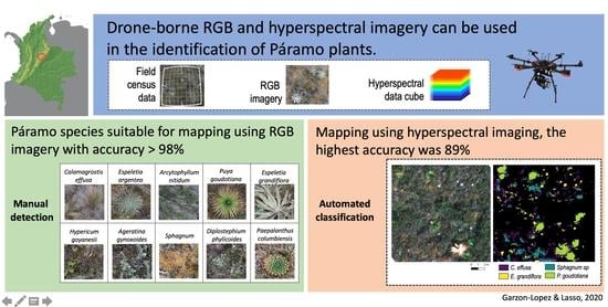
:Páramos host more than 3500 vascular plant species and are crucial water providers for millions of people in the northern Andes. Monitoring species distribution at large scales is an urgent conservation priority in the face of ongoing climatic changes and increasing anthropogenic pressure on this ecosystem. For the first time in this ecosystem, we explored the potential of unoccupied aerial vehicles (UAV)-borne red, green, and blue wavelengths (RGB) and hyperspectral imagery for páramo species classification by collecting both types of images in a 10-ha area, and ground vegetation cover data from 10 plots within this area. Five plots were used for calibration and the other five for validation. With the hyperspectral data, we tested our capacity to detect five representative páramo species with different growth forms using support vector machine (SVM) and random forest (RF) classifiers in combination with three feature selection methods and two class groups. Using RGB images, we could classify 21 species with an accuracy greater than 97%. From hyperspectral imaging, the highest accuracy (89%) was found using models built with RF or SVM classifiers combined with a binary grouping method and the sequential floating forward selection feature. Our results demonstrate that páramo species can be accurately mapped using both RGB and hyperspectral imagery.
1. Introduction
Páramos are located across the highlands of Costa Rica and Panamá down to the northern Andes of Ecuador, Colombia, Venezuela, and Peru [1]. These highly diverse tropical alpine ecosystems provide various services to some of the main capital cities in Latin America, including clean water provision and carbon storage [2], and are an essential reservoir of species with high pharmaceutical potential [3]. Currently, this ecosystem is facing multiple threats that are reducing its surface area. Some of these threats result from unsustainable land use in mining and agriculture, the introduction of invasive plant and animal species, and impacts from climate change [4,5], hence the paramount importance of understanding the vegetation structure, in terms of composition and spatial patterns at multiple scales to ensure its sustainable management and conservation. However, such understanding has been hindered by the inaccessibility and cost of performing surveys at extensions larger than a set of localized plots. While in other ecosystems, remote sensing has shown to be useful for acquiring data at the species-level, particularly high-resolution imagery (<1 m/pixel) in the tropical lowlands [6] and temperate ecosystems [7], in the páramo, the practicality of remote sensing has not yet been thoroughly evaluated.
The potential of remote sensing lies in the ability to provide continuous data at multiple spatial, temporal, and spectral scales, thereby acquiring information on multiple properties of the landscape. Furthermore, it is a tool to inform sampling or as a sampling approach itself in areas where sampling is extremely difficult. Digital imagery in the red, green, and blue wavelengths (henceforth RGB imagery), useful in manual species identification, enables spatial patterns analysis and provides valuable data to inform field sampling design and extend field sampling from already sampled sites to unsampled sites [8]. This technology, thought to be replaced with the newly available thermal and multispectral sensors, continues to be actively used in the development of digital surface models (DSM), animal monitoring (e.g., orangutans and elephants in Malaysia), geological feature assessment (e.g., coastal features) and low-cost agricultural applications [9]. The development of light-weight hyperspectral sensors has increased its medical, agricultural, and environmental applications, as it provides more information on the biochemical structure of surfaces. By measuring reflecting light at hundreds of spectral bands, it allows the detection of subtle differences in leaf composition (e.g., pigments, nutrients, water content) and structure (e.g., size, thickness, shape) from the individual plant scale and at varying degrees of aggregation [10]. Providing detailed information that allows the detection of plant diseases or lack of nutrients and water, invasive plant species, and differentiation of single plant species [11]. This sensor can be mounted on satellites, planes, and unoccupied aerial vehicles (henceforth UAV), with a resulting variation in the spatial resolution of the data and, more importantly, the availability and affordability of each combination sensor(s) vehicle [12] in ecological studies.
Ecological studies have benefited from UAV-borne remote sensing technology, and its potential is thought to have revolutionized ecology and conservation [13], especially in developing countries where research and cost-effective monitoring schemes are urgently needed. However, high ecosystem complexity results in painstaking and costly fieldwork campaigns. UAV-borne RGB and hyperspectral studies have been mostly performed in lowland ecosystems, but recently, increased attention has been placed in highland ecosystems, mainly in Europe, at the alpine grasslands [14]. In the tropical alpine regions of Latin America, the páramo, for example, UAV-borne RGB and multispectral imagery have rarely been used [15,16], and there are no studies using UAV-borne hyperspectral imagery investigating species detection and classification. One possible explanation might be that extracting ecologically meaningful information from hyperspectral data can be complex (i.e., time, computer processing) because it depends on environmental variables that affect the amount of light reflected on the sensor. Likewise, vegetation properties like species diversity and plant size and structure can affect species detection. Tropical alpine ecosystems are characterized by conditions that can hinder our ability to use this new technology; such as high humidity and cloudiness, rough topography, and tremendous diversity of diminutive plant species (around 3500 species), many endemic to the páramo (60% of all species) [1]. Consequently, the combination of spectral band selection and species classification methods to deal with the effect of environmental factors and the high amount of information per pixel (i.e., pixel problem) [17] has a significant effect on the applicability of the hyperspectral images in this setting.
Among the most commonly used species classification methods using hyperspectral data are random forests (RF), support vector machine (SVM) and artificial neural networks (ANN). RF, based on the construction of many decision trees with random subsamples of the training data that are then combined using individual tree votes [18], has successfully been used in land cover and plant species classification [19]. While using SVM, based on a multidimensional feature space where classes are divided using the largest possible separation by applying a kernel function to the training data [20], has resulted in high accuracies, especially in cases of small sample size, and a high number of spectral bands [21]. Moreover, ANN has mostly been used for land cover classification [22]. Raczko and Zagajewski (2017) [23] have compared these three methods for tree species classification and found higher overall accuracy using ANN, but more stability in the overall accuracy using RF and SVM when the sample size is small. A large number of bands increases ANN computational time for model training and testing compared to RF and SVM. Thus, we decided to focus on RF and SVM as our hyperspectral data has a large number of spectral bands and small sample sizes.
In this study, the first one in the páramo ecosystem, we evaluated the potential of RGB and hyperspectral sensors mounted on UAVs for manual (RGB imagery) and supervised (hyperspectral data) species classification. We quantified the accuracy of species detection from RGB imagery using direct observation. From hyperspectral imagery, we identified the reflectance values and evaluated the potential of hyperspectral data to classify individual species using SVM and RF [23,24,25]. All the analyses were performed at the Matarredonda páramo located in the Cruz Verde-Sumapaz páramo system, at the eastern range of the Colombian Andes (Figure 1).
2. Materials and Methods
We explored the potential of RGB and hyperspectral high-resolution UAV-borne data for species classification. To this end, we first evaluated the accuracy in species identification from direct observation of high-resolution RGB images and from the results (Figure 2B), selected the species to be use for the automated classification using hyperspectral data (Figure 2C). Secondly, for hyperspectral imagery, we tested various approaches to build species classification models to assess the potential of hyperspectral images and identify the most appropriate modeling protocol that ensured reliability and replicability (Figure 2D).
2.1. Study Site
The study site is located at Parque Ecológico Matarredonda (4°33′38.1″ N and 74°0′7.3″ W) in the eastern range of the Colombian Andes, which is part of the Cruz Verde-Sumapaz páramo complex (Figure 1). Elevation ranges from 3100 up to 3600 m.a.s.l. The mean annual precipitation is 1178 mm; the mean temperature is 8.8 ºC, and the mean relative humidity is 88% [26]. Matarredonda comprises 690 ha of páramo ecosystem connected to the Cruz Verde-Sumapaz complex and surrounded by a matrix of forest, roads, and agriculture. In this páramo, vegetation is characterized by short and small growth forms composed by rosettes, shrubs, graminoids, forbs, and mosses. The Cruz Verde-Sumapaz complex has 1857 identified plant species. According to previous surveys, Matarredonda has approximately 30 vascular plant species [27]. However, our annual census has counted more than 97 species, including two the emblematic species in the genus Espeletia, Espeletia argentea, and Espeletia grandiflora [28]. Three soil orders have been found in Matarredonda; inceptisols, histosols and entisols that evidence high humidity levels and organic concentration and reveal past agricultural land use [29].
2.2. Spectral and Field Data
RGB and hyperspectral data for a 10 ha polygon were taken. RGB data were collected with a camera FC6310 (8.8 mm) mounted on a DJ Phantom Pro drone set at a flying altitude of 79.5 m, which resulted in a set of 94 images with 1 cm pixel resolution. Hyperspectral data were collected with sensor 1003A-20502: Hyperspec Nano VNIR (400–1000 nm with a band width of 2.2 nm), with lenses 1004A-21444: F/1.4, 400–1000 nm, compact barrel, C-Mount, 17 mm, Global Positioning System (GPS), Inertial Motion Unit (IMU), and fiber-optic downwelling irradiance sensor (fodis unit) mounted on the UAS-ART Unmounted Aerial Vehicle (UAV) DJI Matrice 600 Pro. The flying altitude was 118 m and resulted in a total of 4 strips (henceforth images A, B, C, and D in Table 1) of 272 spectral bands with 3 cm pixel resolution covering an area of ~1738 m2 each image.
Field data were collected from 10 previously established, permanent plots (1 m × 1 m each), part of an ongoing vegetation experiment, where each plant on the plot has been identified to the species or genus level, and their position has been registered (projection system WGS 84). An additional field campaign was performed to add a 100 m2 vegetation ground survey around the plots, to include more individuals per species of the 40 species that we manually identified on the RGB imagery based on the 1 m2 plot vegetation data.
RGB data were georeferenced and orthorectified using GRASS GIS software. Hyperspectral data were processed using the Hyperspec III software (Headwall Photonics Inc. Fitchburg, MA, USA) that synchronizes the image cubes with the GPS/IMU data to allow orthorectification. In succession, we transformed the raw image cube digital numbers (DN) to radiance and reflectance values using the real-time solar radiance collected in the fodis unit in the SpectralView software (Headwall Photonics Inc. Fitchburg, MA, USA).
2.3. RGB Imagery Analysis—Manual Detection
To evaluate the RGB images’ applicability to identify páramo species, we used a manual training and testing approach. At the training 1 m2 plots, we used the ground locations to join the point location to its crown shape in the RGB image. However, since the plot’s area was too small to include more than a couple of individuals per species, we performed another ground survey in the 100 m2 around each plot, collecting the XY location of individuals of the species already matched in the 1x1 m plot. This step increased the training and testing area to 100 m2 which was used to develop the identification key and perform the tests.
At the 100 m2 training areas, characteristics such as growth form (e.g., rosette, grass, shrub), color and size, were used to develop an identification key for each species in the RGB image correctly matched the ground XY location data. The key consisted of a page with a collection of cropped images of the focal species and a written classification of its size, color, and growth form. The key was then used to help 2 trained observers consistently map species in the field, dropping a point with the species ID on a newly created vector file. Then, the identification in the test vector file was revised, comparing ground data points collected with the GPS, and evaluating the results using a confusion matrix and accuracy statistics (Figure 2B). All the analyses were performed using QGIS software [30].
2.4. Hyperspectral Data Analysis—Automated Classification
For the hyperspectral data, we used five of the species correctly identified from the RGB imagery to select at least five individuals per species in each plot and each of the images to perform the classification. Table 1 summarizes the datasets used for each species and image.
The hyperspectral data contained 262 spectral bands (400–1000 nm—band width 2.2 nm). Feature selection is commonly used for this type of data to select spectral bands with the highest prediction ability [18]. We used three feature selection methods: (1) all spectral bands, (2) the spectral bands with the highest importance based on the RF mean decrease in Gini values, and (3) features selected using the sequential floating forward selection (SFFS). For method (2), the spectral bands with the highest importance were identified based on the random forest mean decrease in Gini values, which calculates the importance of each spectral band as a measurement of the purity of class samples gain in each individual RF tree split. For method (3), the bands with the highest spectral separability were identified using SFFS, based on a Gaussian mixture model (GMM) classifier, that selects bands through back and forward iteration until it identifies the bands with the highest spectral separability base on the Jeffries-Matusita distance [18].
To investigate the effect of an approach using a single focal species vs. an approach with multiple focal species, we tested two class-grouping methods: (1) binary training data were divided into focal species class and non-focal species class and, (2) multiple training data were divided into 4 to 5 classes corresponding to each of the focal species present in the image.
The RF classifier is a robust method, especially dealing with complex highly-colinear variables, such as hyperspectral bands, where it has been used to identify various types of landcover, from invasive plant species to crop types [31,32,33,34,35]. In this study, the RF classifier was used with two purposes, to assess the importance of the variables via the Gini index and to perform the image classification. The SVM classifier is a non-parametric free classifier [36] that has been used successfully in hyperspectral image classification [6,18] (Figure 2D).
A dataset was built extracting pixel values for each spectral band of each individual plant in the sample. The dataset was divided into two random sample partitions using the createDataPartition command in the R package caret [37] that divides the dataset into two groups of pixel values while preserving its class distribution; in this case, the number of pixels per species. The resulting datasets consisted of a training sample from 40% of the total data and a testing sample with the remaining 60%. Additionally, to test the effect of the data partition used (per pixel partition vs. per sample partition), we divided the data for images C and D, which have the highest number of individuals sampled, into training and testing samples. The training data for C and D consisted of 40% of the individuals randomly selected and the testing sample had the remaining 60% of the individuals.
The classification models were compared using the same training and test samples. To assess model performance and perform parameter tuning, we evaluated two approaches. The random cross-validation approach does not include spatial autocorrelation, and the spatial validation approach includes the effect of spatially autocorrelated spectral bands in the dataset. For cross-validation, a subsample of the data was left out to test the trained model’s performance using the rest of the training data. This process was repeated ten times, and the average of all the tests was used to estimate model performance [38]. For spatial validation, model performance was evaluated using spatial blocks, that is, equally sized polygons dividing the image. Model performance was repeatedly (ten times) tested using the data from all the spatial blocks but one, and the average of all the tests was used to estimate model performance [39].
Finally, the accuracy of all the combinations of selection and classification approaches was assessed using the testing dataset, to calculate overall accuracy (OA), Kappa accuracy (KA), specificity (SP), and sensitivity (SE) for each species. All the analyses were performed using the R software [40]. For the implementation in R of the caret package, we used the raster [41] and randomForest [42] packages, and for the feature selection process we used kernlab [43], varSel [44] and sf [45].
3. Results
3.1. Manual Species Identification Using RGB Imagery
From the 97 species registered in the ground survey, 40 species were identified in the aerial images. From the identified species, we selected the ones from which at least five individuals in the training areas were correctly identified, to include variation in the species typology (shape, color, texture), which resulted in 21 species that were then searched for in the test plots. For these 21 species, accuracy was above 97%, while omission error ranged between 1.49 and 87.5. For 12 of those species, omission error was above 10% and up to 87%, showing that these species were difficult to see in the images (false absences). However, if they were spotted, they could be correctly identified with at least 97% accuracy (Table 2, Figure 3). The species with the highest accuracies, precision values, and lowest commission errors corresponded to large rosettes (E. grandiflora, E. argentea, and P. goudotiana), dense clumps (Sphagnum sp.), and common in the study area (C. effusa and H. goyanesis). These species were selected to perform the automated classification using hyperspectral imagery (Figure 2B).
3.2. Automated Species Classification Using Hyperspectral Data
The selected spectral bands using SFFS and RF approach were spread across the spectrum with two clusters located between 420 and 630 nm, 735 and 840 nm. Different bands were selected for each image, with marked differences in image A and RF feature selection, for which the selected bands are between 550 and 800 nm (Figure 4). The most considerable differences in spectral values among species are located in the NIR zone of the spectrum, where the rosette P. goudotiana has the highest reflectance percentage values while the grass C. effusa has the lowest. These differences are likely to be related to the larger proportion of necromass that usually surrounds grasses compared to the green foliage of the bromeliads. The spectral signature of two species of the same genus, E. grandiflora and E. argentea, important endemic species of the páramo ecosystem, can be visually differentiated with higher reflectance percentage for E. argentea in the visible range in comparison with E. grandiflora, while the NIR zone E.grandiflora shows higher values than E. argentea (Figure 4).
Of all the classification methods, the combination of two classes (binary), all bands feature selection, SVM classifier, and random cross-validation obtained the highest overall accuracy percentage (91%), followed by the same combination using the RF classifier (90%) (Figure 5). Overall accuracy was also higher when using two classes (mean 85%) than when including multiple classes (mean 68%), but the differences in the number of samples for the two classes decrease the accuracy to a kappa accuracy mean value of 50%, while it remained higher when using multiple classes (mean 67%). The RF method had, in general, higher overall accuracy values than SVM, and both classifiers were affected by the feature selection method, with higher overall and kappa accuracy values for feature selection using the SFFS classifier compared to RF (Figure 5).
As presented in Figure 6, overall and kappa accuracy were similar across images when all the bands were included, independent of the number of classes or the classifiers used. However, when a feature selection method was applied (SFFS or RF), lower overall and kappa accuracy values were observed (SFFS > RF) accompanied with a higher variation between images. This pattern was especially visible when features were selected using RF.
Regarding sensitivity and specificity, four of the five species studied (C. effusa, E. argentea, E. grandiflora, and Sphagnum sp.) had higher true negative rate (specificity > 96%) in models constructed from two classes, while the true-positive rate (sensitivity > 53%) was higher for models constructed from multiple classes. The fifth species, P. goudotiana, presented the opposite pattern where higher true-positive rates were found in the models constructed from binary classes, while higher true negative rates were found in the multiple class models (Table 3). Nevertheless, the models with relatively higher sensitivity and specificity were models with binary classes, the SVM classifier in the case of C. effusa, E. argentea, Sphagnum sp., and E. grandiflora. In general, the models constructed using all bands showed the highest specificity (>96%) rates, followed by the models using SFFS feature selection (specificity ± 95%). Spatial cross-validation significantly reduced the sensitivity rates for four of the species studied (C. effusa < 10%, E. argentea < 10%, E. grandiflora < 27%, and Sphagnum sp. < 23%) except for P. goudotiana (<77%). Notably, the highest specificity values for spatial cross-validation were from models constructed using the RF feature selection method and binary classes.
Regarding data partition, the overall accuracy was reduced when using the per individual data partition approach. However, the effect was smaller for the approaches using the binary classes, particularly in combination with the SVM classifier where the variation in accuracy was higher. In comparison, the effect was more substantial when using the multiple classes approach, especially in combination with the RF classifier (Supp. Figure S1).
4. Discussion
4.1. Manual Species Identification Using RGB Imagery
Our study demonstrated the importance of RGB images for low-cost páramo species mapping and monitoring. Despite the size of the study area that limited the number of individuals per species we could use for training and testing, we were able to identify 41% of the species found in this ecosystem and evaluate the accuracy of 20 species with accuracy levels above 97%. Many páramo species were often not visible from the RGB image because of their small size and because they are often covered by larger species (e.g., shrubs, large rosettes). However, here we found that it was relatively easy to correctly identify some of them thanks to its conspicuous structure (Diplostepihum phylicoides) or the large patches they form (Sphagnum sp.). Higher resolution (<1 cm) might allow reducing the omission errors observed in this study as we observed it in preliminary higher resolution (1 cm pixel) RGB images.
Despite the high diversity of short-stature growth forms and the large proportion of cloudy and rainy days throughout the year, acquiring the images was feasible. It only required a couple of hours of clear sky to obtain 1cm pixel-resolution used in this study. Previous research has highlighted the importance of this type of imagery in different types of ecosystems from big trees in highly diverse tropical [46,47] and subtropical forests [48], to small stature species in temperate grasslands [49], in a diverse set of ecological studies that include mapping, restoration and monitoring [50,51,52]. In this study, we conclude that high-resolution imagery (1 cm pixel) has great potential for at least 21% of the species, comprising a range of growth forms from big rosettes (P. goudotiana), endemic species (Espeletia sp.) to mosses (Sphagnum sp.), that are known to be essential in this ecosystem [53,54,55]. Such an outcome shows the potential of UAV-borne RGB imagery for low-cost, in terms of time and money, efforts to visually detect changes in the species composition and enhance ground surveys and inform the development of the automated image classification techniques explored in this study.
4.2. Automated Species Identification Using Hyperspectral Data
Our study has shown that hyperspectral data effectively differentiated five important páramo species, two of them of the same genus and endemic from this ecosystem, following other studies in temperate alpine ecosystems [49,50]. Comparing overall model accuracy, combining two classes (binary), all bands and the SVM classifier had high accuracy, followed closely by the model developed using binary classes, SFFS for feature selection, and SVM or RF classifiers (Figure 7). Our results agree with Burai et al. 2015 [56], a study performed on the vegetation of similar characteristics (herbaceous), where, using all the bands, SVN performed slightly better than RF, but the differences were not significant [50]. Additionally, they found that the number of pixels affected the classification accuracy, which was similar to our results at the species level (P. goudotiana, 15,724 pixels, Supp. Figure S2) but not at the image level. In our study, the image with the highest number of pixels (image A, 20,084 pixels) did not have the highest overall accuracy values, reflecting that the characteristics of the image such as the spatial distribution of the classes affects the accuracy independent of the number of pixels (Figure 6).
Sensitivity and specificity were also higher for all bands, binary classes, and SVM model combinations for all the species classified. When comparing overall and kappa accuracies across images, the RF classifier showed more inconsistencies than the SVM classifier, and the SVM classifier had higher accuracy values for all images than the RF classifier. This finding is relevant for monitoring schemes, where multiple images are taken at different points in time, in which case the SVM classifier is more stable despite differences in the hyperspectral data, and has more consistency. Regarding the data partition, in cases where the sample size is small, and the per-pixel partition is used, we recommend using the binary classes in combination with the SVM classifier. Doing so would result in more consistent outcomes, in terms of variation and decreases in the overall accuracy, when comparing both data partition approaches. This difference in consistency suggests that the combination of binary classes and SVM classifier might be less affected by the effect of autocorrelation among pixels, probably because of a lower number of classes involved in the determination of the separating margin with kernel methods. Nevertheless, including high-resolution RGB imagery and visual classification for developing individual species sample, as we did in our study, increases the number of individuals identified, hence sample size. In our particular case, increasing the RGB imagery resolution would have significantly improved our sample size.
Upon visual examination of the classified maps, the results were not as expected, given the high accuracy values, especially in images with small aggregations of the species studied. On the one hand, species classification methods using a pixel-based approach are prone to inflated accuracy values due to autocorrelated pixel values. On the other hand, the data are collected within a spatial context, and therefore the effect of space should also be included in order to construct models relevant across the landscape. Following Meyer et al. 2019, including space, using spatial cross-validation, resulted in more variation in the overall accuracy and kappa values [39]. Additionally, we found that this effect is more substantial in the models constructed using multiple classes, as in the binary classes, overall accuracy did not vary significantly from the random cross-validation. According to our results, binary models appear to be more suited for species with a highly aggregated spatial distribution because it increases the number of non-focal samples, thereby increasing the accuracy in areas where the number of individuals of the focal species is low. For P. goudotiana, the true negative rate did not decrease as much as for the other species; this might be related to the plant size (e.g., a higher number of pixels), but the true positive rate was affected, which might be due to the dense spatial aggregation of this species. Our study demonstrates the potential of hyperspectral images for species classification in tropical alpine ecosystems, in accordance with the findings from Marcinkowska-Ochtyra et al. 2018 [14], but in their study, the SVM classifier performed better with a subset of 40 bands, whereas in our analysis, it performed slightly better when using all bands.
Hennessy et al. (2020) [57], in their review on the hyperspectral classification of plants, highlighted the importance of testing multiple feature selection and classification methods due to the high variation in outcomes among studies. Out study supports this statement. We found that the values of accuracy, kappa, sensitivity, and specificity varied depending on the species and image analyzed and the combination of feature selection, number of classes, and classifier applied.
From our results, the potential of RGB and hyperspectral imagery for species classification at the páramo is relevant, and the advantages of each technology make them better when used together. On the one hand, the low-cost RGB imagery approach allows for higher accuracies with lower computer processing requirements, but has higher omission rate and can be time-consuming when mapping large areas. Classification using hyperspectral imagery, although requiring more computer processing, reaches stable overall accuracies above 75% (when using binary classes, SVM or RF classifiers and all bands) in a fraction of the time required using RGB imagery. However, the combination of both can give the best results as we show in this study where we have taken advantage of the RGB imagery to identify plant species that could be used to develop the automated hyperspectral image classification. Thus, RGB imagery appears promising to monitor several páramo plant species while providing data to develop automated classification with hyperspectral images for a subset of the species.
5. Conclusions
In this study, we explored the potential of UAV-borne RGB and hyperspectral imagery for species classification in one type of tropical alpine ecosystem (páramo). Our results regarding species identification using RGB imagery highlight the importance of this low-cost technology as a useful tool for vegetation monitoring in this ecosystem, especially given that all the analyses were performed using free and open source software (FOSS), which keeps the costs down and facilitates applicability. However, given the high omission error due to the small vegetation sizes, characteristic of tropical alpine plant communities, we propose the use of higher resolution images, which would not significantly increase flying time but rather increase species identification performance.
Hyperspectral automated species classification, using a combination of multiple feature selection methods, data partition, classifiers, number of classes, and cross-validation approaches, allowed us to explore the potential of hyperspectral for páramo species classification thoroughly. Even though the pixel resolution used in this study allowed us to perform all the analysis, exploring the spatial resolution would provide insight into the resolution thresholds needed for an accurate species classification. Future directions should also include a test of the effect of larger samples on the model performance and the spatial arrangement of those samples to include the effect of spatial distribution patterns of the species in the classification process.
The páramo ecosystem is highly threatened by land-use change, plant invasions, and climate change; thus, this technology’s potential to help understand, monitor, and detect threats at the landscape scale opens a promising alternative to species management and conservation in tropical alpine regions. RGB imagery and hyperspectral data offer several advantages to monitor changes in species survival and distribution patterns. RGB imagery can be used for annual monitoring of selected areas, and hyperspectral imagery can be applied for five-year monitoring at the landscape-level, with the advantage of all the other well-known applications of these data (e.g., biochemical signals of change and invasive species detection). Future directions could build from this method and explore plant trait mapping using UAV-borne hyperspectral images, monitor individuals and changes in spatial distribution patterns and explore the transferability of these methods to other páramos.
Supplementary Materials
The following are available online at https://www.mdpi.com/2504-446X/4/4/69/s1, Figure S1: Variation in model performance per data partition approach (per pixels, and per individual) in terms of overall accuracy (for spatial and random cross-validation) given the combination of feature selection, class grouping method (Binary or Multiple) and classification method (Random forest (RF) and Support vector machine (SVM). In the case of feature selection: all the spectral bands (ALL), spectral bands selected using Sequential Floating Forward Selection (SFFS) using Jeffries-Matusita distance as a separability index (FSSF) and, spectral bands with the highest importance on random forest the Gini decrease mean value (RF), Figure S2: Variation in model performance per species in terms of producer accuracy (for spatial and random cross-validation) given the combination of feature selection, class grouping method (Binary or Multiple) and classification method (Random forest (RF) and Support vector machine (SVM). In the case of feature selection: all the spectral bands (ALL), spectral bands selected using Sequential Floating Forward Selection (SFFS) using Jeffries-Matusita distance as a separability index (FSSF) and, spectral bands with the highest importance on random forest the Gini decrease mean value (RF).
Author Contributions
Conceptualization C.X.G.-L.; Data processing and analysis, C.X.G.-L.; writing, reviewing and editing, C.X.G.-L. and E.L. All authors have read and agreed to the published version of the manuscript.
Funding
This research was funded by University of los Andes: “Fondo de Investigaciones para apoyar programas de profesores de la Facultad de Ciencias de la Universidad de los Andes, grant number INV-2019-84-1805 and by Colciencias Patrimonio autónomo fondo nacional de financiamiento para la ciencia, la tecnología y la innovación Francisco José de Caldas”, grant number 120471451294.
Acknowledgments
Special thanks to all the people that helped collecting data in the field: Alejandra Ayarza, Indira Leon, Lina Aragon, Paola Matheus, Marisol Cruz, David Ocampo. We would like to thank the Sabogal family for allowing us to establish the plots and fly the drone in the “Parque Ecológico Matarredonda”. Special thanks to Michele Dalponte for his valuable advice on the data analysis.
Conflicts of Interest
The authors declare no conflict of interest.
References
- Madriñán, S.; Cortés, A.J.; Richardson, J.E. Páramo is the world’s fastest evolving and coolest biodiversity hotspot. Front. Genet. 2013, 4, 192. [Google Scholar] [CrossRef] [PubMed] [Green Version]
- Farley, K.A.; Bremer, L.L.; Harden, C.P.; Hartsig, J. Changes in carbon storage under alternative land uses in biodiverse Andean grasslands: Implications for payment for ecosystem services. Conserv. Lett. 2013, 6, 21–27. [Google Scholar] [CrossRef]
- Bueno, J.; Ritoré, S. Bioprospecting Model for a New Colombia Drug Discovery Initiative in the Pharmaceutical Industry. In Analysis of Science, Technology, and Innovation in Emerging Economies; Martínez, C.I.P., Poveda, A.C., Moreno, S.P.F., Eds.; Springer International Publishing: Cham, Switzerland, 2019; pp. 37–63. [Google Scholar]
- Balthazar, V.; Vanacker, V.; Molina, A.; Lambin, E.F. Impacts of forest cover change on ecosystem services in high Andean mountains. Ecol. Indic. 2015, 48, 63–75. [Google Scholar] [CrossRef]
- Buytaert, W.; Celleri, R.; de Bievre, B.; Cisneros, F.; Wyseure, G.; Deckers, J.; Hofstede, R. Human impact on the hydrology of the Andean páramos. Earth-Sci. Rev. 2006, 79, 53–72. [Google Scholar] [CrossRef]
- Baldeck, C.A.; Asner, G.P.; Martin, R.E.; Anderson, C.B.; Knapp, D.E.; Kellner, J.R.; Wright, S.J. Operational Tree Species Mapping in a Diverse Tropical Forest with Airborne Imaging Spectroscopy. PLoS ONE 2015, 10, e0118403. [Google Scholar] [CrossRef]
- He, K.S.; Rocchini, D.; Neteler, M.; Nagendra, H. Benefits of hyperspectral remote sensing for tracking plant invasions: Plant invasion and hyperspectral remote sensing. Divers. Distrib. 2011, 17, 381–392. [Google Scholar] [CrossRef]
- Garzon-Lopez, C.X.; Bohlman, S.A.; Olff, H.; Jansen, P.A. Mapping Tropical Forest Trees Using High-Resolution Aerial Digital Photographs. Biotropica 2013, 45, 308–316. [Google Scholar] [CrossRef] [Green Version]
- Colomina, I.; Molina, P. Unmanned aerial systems for photogrammetry and remote sensing: A review. ISPRS J. Photogramm. Remote Sens. 2014, 92, 79–97. [Google Scholar] [CrossRef] [Green Version]
- Thenkabail, P.S.; Lyon, J.G.; Lyon, J.G. Hyperspectral Remote Sensing of Vegetation; CRC Press: Boca Raton, FA, USA, 2016. [Google Scholar]
- Yao, H.; Qin, R.; Chen, X. Unmanned Aerial Vehicle for Remote Sensing Applications—A Review. Remote Sens. 2019, 11, 1443. [Google Scholar] [CrossRef] [Green Version]
- Warner, T.A.; Nellis, M.D.; Foody, G.M. Remote Sensing Scale and Data Selection Issues. In The SAGE Handbook of Remote Sensing; SAGE Publications, Inc.: Oliver’s Yard, London, UK, 2009; pp. 2–17. [Google Scholar]
- Ewald, M.; Skowronek, S.; Aerts, R.; Lenoir, J.; Feilhauer, H.; van de Kerchove, R.; Honnay, O.; Somers, B.; Garzon-Lopez, C.X.; Rocchini, D.; et al. Assessing the impact of an invasive bryophyte on plant species richness using high resolution imaging spectroscopy. Ecol. Indic. 2020, 110, 105882. [Google Scholar] [CrossRef]
- Marcinkowska-Ochtyra, A.; Zagajewski, B.; Raczko, E.; Ochtyra, A.; Jarocińska, A. Classification of High-Mountain Vegetation Communities within a Diverse Giant Mountains Ecosystem Using Airborne APEX Hyperspectral Imagery. Remote Sens. 2018, 10, 570. [Google Scholar] [CrossRef] [Green Version]
- Martín, L.D.; Medina, J.; Upegui, E. Assessment of Image-Texture Improvement Applied to Unmanned Aerial Vehicle Imagery for the Identification of Biotic Stress in Espeletia. Case Study: Moorlands of Chingaza (Colombia). Cienc. E Ing. Neogranadina 2020, 30, 27–44. [Google Scholar] [CrossRef]
- Martínez, E. Análisis de la Respuesta Espectral de las Coberturas Vegetales de los Ecosistemas de Páramo Y Humedales a Partir de los Sensores Aerotransportados Ultracam D, Dji Phanton 3 Pro Y Mapir Nir. Casos de estudio humedal “El ocho”, Villamaria – Caldas. Master’s Thesis, Universidad Católica de Manizales, Caldas, Colombia, 2017. [Google Scholar]
- Abe, B.T.; Olugbara, O.O.; Marwala, T. Experimental comparison of support vector machines with random forests for hyperspectral image land cover classification. J. Earth Syst. Sci. 2014, 123, 779–790. [Google Scholar] [CrossRef]
- Dalponte, M.; Ørka, H.O.; Gobakken, T.; Gianelle, D.; Næsset, E. Tree Species Classification in Boreal Forests with Hyperspectral Data. IEEE Trans. Geosci. Remote Sens. 2013, 51, 2632–2645. [Google Scholar] [CrossRef]
- Rodriguez-Galiano, V.F.; Ghimire, B.; Rogan, J.; Chica-Olmo, M.; Rigol-Sanchez, J.P. An assessment of the effectiveness of a random forest classifier for land-cover classification. ISPRS J. Photogramm. Remote Sens. 2012, 67, 93–104. [Google Scholar] [CrossRef]
- Sluiter, R.; Pebesma, E.J. Comparing techniques for vegetation classification using multi- and hyperspectral images and ancillary environmental data. Int. J. Remote Sens. 2010, 31, 6143–6161. [Google Scholar] [CrossRef]
- Mountrakis, G.; Im, J.; Ogole, C. Support vector machines in remote sensing: A review. ISPRS J. Photogramm. Remote Sens. 2011, 66, 247–259. [Google Scholar] [CrossRef]
- Petropoulos, G.P.; Kontoes, C.C.; Keramitsoglou, I. Land cover mapping with emphasis to burnt area delineation using co-orbital ALI and Landsat TM imagery. Int. J. Appl. Earth Obs. Geoinf. 2012, 18, 344–355. [Google Scholar] [CrossRef]
- Raczko, E.; Zagajewski, B. Comparison of support vector machine, random forest and neural network classifiers for tree species classification on airborne hyperspectral APEX images. Eur. J. Remote Sens. 2017, 50, 144–154. [Google Scholar] [CrossRef] [Green Version]
- Pal, M.; Mather, P.M. Assessment of the effectiveness of support vector machines for hyperspectral data. Future Gener. Comput. Syst. 2004, 20, 1215–1225. [Google Scholar] [CrossRef]
- Shadman Roodposhti, M.; Aryal, J.; Lucieer, A.; Bryan, B.A. Uncertainty Assessment of Hyperspectral Image Classification: Deep Learning vs. Random Forest. Entropy 2019, 21, 78. [Google Scholar] [CrossRef] [Green Version]
- Leon-Garcia, I.V.; Lasso, E. High heat tolerance in plants from the Andean highlands: Implications for paramos in a warmer world. PLoS ONE 2019, 14, e0224218. [Google Scholar] [CrossRef] [Green Version]
- Madriñán, S.; Navas, A.; Garcia, M.W. Páramo Plants Online: A Web Resource to Study Páramo Plant Distributions, Dec. 2016. Available online: http://paramo.uniandes.edu.co/V3/ (accessed on 20 August 2020).
- Ariza Cortes, W. Caracterización Biótica del Complejo de Páramos Cruz Verde-Sumapaz en Jurisdicción de la CAM, CAR, CORMACARENA, CORPOORINOQUIA y la SDA; Instituto Alexander von Humboldt, Universidad Distrital Francisco Jose de Caldas: Columbia, Colombia, 2013. [Google Scholar]
- Rodriguez, C.R.R.; Duarte, C.; Ardila, J.O.G. Estudio de suelos y su relación con las plantas en el páramo el verjón ubicado en el municipio de choachí Cundinamarca. TECCIENCIA 2012, 6, 56–72. [Google Scholar]
- QGIS Development Team. QGIS Geographic Information System. Open Source Geosp. Found. Project 2020. [Google Scholar]
- Breiman, L. Random Forests. Mach. Learn. 2001, 45, 5–32. [Google Scholar] [CrossRef] [Green Version]
- Amini, S.; Homayouni, S.; Safari, A.; Darvishsefat, A.A. Object-based classification of hyperspectral data using Random Forest algorithm. Geo-Spat. Inf. Sci. 2018, 21, 127–138. [Google Scholar] [CrossRef] [Green Version]
- Belgiu, M.; Drăguţ, L. Random forest in remote sensing: A review of applications and future directions. ISPRS J. Photogramm. Remote Sens. 2016, 114, 24–31. [Google Scholar] [CrossRef]
- Lawrence, R.L.; Wood, S.D.; Sheley, R.L. Mapping invasive plants using hyperspectral imagery and Breiman Cutler classifications (randomForest). Remote Sens. Environ. 2006, 100, 356–362. [Google Scholar] [CrossRef]
- Salas, E.A.L.; Subburayalu, S.K. Modified shape index for object-based random forest image classification of agricultural systems using airborne hyperspectral datasets. PLoS ONE 2019, 14, e0213356. [Google Scholar] [CrossRef]
- Cortes, C.; Vapnik, V. Support-vector networks. Mach. Learn. 1995, 20, 273–297. [Google Scholar] [CrossRef]
- Kuhn, M. Caret: Classification and Regression Training, R Package Ver. 6.0; R Core Team: Vienna, Austria, 2020. [Google Scholar]
- Kuhn, M.; Johnson, K. Applied Predictive Modeling; Springer: New York, NY, USA, 2013. [Google Scholar]
- Meyer, H.; Reudenbach, C.; Wöllauer, S.; Nauss, T. Importance of spatial predictor variable selection in machine learning applications—Moving from data reproduction to spatial prediction. Ecol. Model. 2019, 411, 108815. [Google Scholar] [CrossRef] [Green Version]
- Chambers, J. Software for Data Analysis. Programming with R; Springer: New York, NY, USA, 2008. [Google Scholar]
- Hijmans, R.J. Raster: Geographic Data Analysis and Modeling, R Package Ver. 3.3; R Core Team: Vienna, Austria, 2020. [Google Scholar]
- Liaw, A.; Wiener, M. Classification and Regression by randomForest. R News 2002, 2, 18–22. [Google Scholar]
- Karatzoglou, A.; Smola, A.; Hornik, K.; Zelleis, A. Kernlab—An S4 Package for Kernel Methods in R. J. Stat. Softw. 2004, 11, 1–20. [Google Scholar] [CrossRef] [Green Version]
- Dalponte, M.; Oerka, H.O. VarSel: Sequential Forward Floating Selection Using Jeffries-Matusita Distance, R Package Ver. 0.1; R Core Team: Vienna, Austria, 2016. [Google Scholar]
- Edzer, P. Simple Features for R: Standardized Support for Spatial Vector Data. R J. 2018, 10, 439–446. [Google Scholar] [CrossRef] [Green Version]
- Park, J.Y.; Muller-Landau, H.C.; Lichstein, J.W.; Rifai, S.W.; Dandois, J.P.; Bohlman, S.A. Quantifying Leaf Phenology of Individual Trees and Species in a Tropical Forest Using Unmanned Aerial Vehicle (UAV) Images. Remote Sens. 2019, 11, 1534. [Google Scholar] [CrossRef] [Green Version]
- Waite, C.E.; van der Heijden, G.M.F.; Field, R.; Boyd, D.S. A view from above: Unmanned aerial vehicles (UAVs) provide a new tool for assessing liana infestation in tropical forest canopies. J. Appl. Ecol. 2019, 56, 902–912. [Google Scholar] [CrossRef]
- Zhang, J.; Hu, J.; Lian, J.; Fan, Z.; Ouyang, X.; Ye, W. Seeing the forest from drones: Testing the potential of lightweight drones as a tool for long-term forest monitoring. Biol. Conserv. 2016, 198, 60–69. [Google Scholar] [CrossRef]
- Sun, Y.; Yi, S.; Hou, F. Unmanned aerial vehicle methods makes species composition monitoring easier in grasslands. Ecol. Indic. 2018, 95, 825–830. [Google Scholar] [CrossRef]
- Woellner, R.; Wagner, T.C. Saving species, time and money: Application of unmanned aerial vehicles (UAVs) for monitoring of an endangered alpine river specialist in a small nature reserve. Biol. Conserv. 2019, 233, 162–175. [Google Scholar] [CrossRef]
- Cruzan, M.B.; Weinstein, B.G.; Grasty, M.R.; Kohrn, B.F.; Hendrickson, E.C.; Arredondo, T.M.; Thompson, P.G. Small unmanned aerial vehicles (micro-UAVs, drones) in plant ecology. Appl. Plant. Sci. 2016, 4, 1600041. [Google Scholar] [CrossRef]
- Tay, J.Y.L.; Erfmeier, A.; Kalwij, J.M. Reaching new heights: Can drones replace current methods to study plant population dynamics? Plant. Ecol. 2018, 219, 1139–1150. [Google Scholar] [CrossRef]
- Cortés, A.J.; Garzón, L.N.; Valencia, J.B.; Madriñán, S. On the Causes of Rapid Diversification in the Páramos: Isolation by Ecology and Genomic Divergence in Espeletia. Front. Plant. Sci. 2018, 9, 1700. [Google Scholar] [CrossRef]
- Jabaily, R.S.; Sytsma, K.J. Historical biogeography and life-history evolution of Andean Puya (Bromeliaceae). Bot. J. Linn. Soc. 2013, 171, 201–224. [Google Scholar] [CrossRef] [Green Version]
- Merchán-Gaitán, J.B.; Álvarez-Herrera, J.G.; Delgado-Merchán, M.V. Retención de agua en musgos de páramo de los municipios de Siachoque, Toca y Pesca (Boyacá). Rev. Colomb. Cienc. Hortícolas 2011, 5, 295–302. [Google Scholar] [CrossRef] [Green Version]
- Burai, P.; Deák, B.; Valkó, O.; Tomor, T. Classification of Herbaceous Vegetation Using Airborne Hyperspectral Imagery. Remote Sens. 2015, 7, 2046–2066. [Google Scholar] [CrossRef] [Green Version]
- Hennessy, A.; Clarke, K.; Lewis, M. Hyperspectral Classification of Plants: A Review of Waveband Selection Generalisability. Remote Sens. 2020, 12, 113. [Google Scholar] [CrossRef] [Green Version]
Figure 1.
Map of the study area (10 ha) with vegetation plot locations. Páramo de Matarredonda located in the eastern range of the Colombian Andes.
Figure 1.
Map of the study area (10 ha) with vegetation plot locations. Páramo de Matarredonda located in the eastern range of the Colombian Andes.

Figure 2.
Workflow for species manual detection using red, green, and blue wavelengths (RGB) (B) and automated classification using Hyperspectral data, including preprocessing (C) and automated classification (D). Boxes in dashed lines (A) correspond to input data.
Figure 2.
Workflow for species manual detection using red, green, and blue wavelengths (RGB) (B) and automated classification using Hyperspectral data, including preprocessing (C) and automated classification (D). Boxes in dashed lines (A) correspond to input data.

Figure 3.
Aerial photographs of 10 plant species in Matarredonda that may be suitable for drone mapping. Accuracies for all species are above 98%. Values correspond to the percentage of omission errors for the five testing plots.
Figure 3.
Aerial photographs of 10 plant species in Matarredonda that may be suitable for drone mapping. Accuracies for all species are above 98%. Values correspond to the percentage of omission errors for the five testing plots.

Figure 4.
Mean and 95% confidence intervals of the reflectance spectra for the 5 species (>30 individuals per species) included in the species classification models and the spectral bands selected by the two feature selection methods used: random forest (RF) and forward selection (SFFS) for each image (A, B and C).

Figure 5.
Variation in model performance in terms of overall accuracy and kappa accuracy given the combination of feature selection, class grouping method (Binary or Multiple), classification method (Random forest (RF) and Support vector machine (SVM)), and cross-validation method (Random, Spatial). In the case of feature selection: all the spectral bands (ALL), spectral bands selected using Sequential Floating Forward Selection (SFFS) using Jeffries–Matusita distance as a separability index (FSSF) and, spectral bands with the highest importance on random forest the Gini decrease mean value (RF).

Figure 6.
Variation in model performance, using random cross-validation, in terms of overall and kappa accuracy values for each of the images analyzed (A, B and C) and for all combinations of model construction: feature selection using all bands (ALL), bands selected with fast forward selection (SFFS) and bands selected using the Gini decrease index in random forest (RF), number of classes from two classes (binary) to five classes (multiple) and with two modeling approaches namely random forest (RF) and support vector machine (SVM).

Figure 7.
Example of classification results using binary classes, sequential fast forward feature selection (SFFS) and SVM classifier, compared to the view from a false color representation of the hyperspectral data for C. effusa, E. grandiflora, Sphagnum, P. goudotiana.
Figure 7.
Example of classification results using binary classes, sequential fast forward feature selection (SFFS) and SVM classifier, compared to the view from a false color representation of the hyperspectral data for C. effusa, E. grandiflora, Sphagnum, P. goudotiana.


Table 1.
Summary of individuals mapped and validated in the field with its corresponding spectral data for each of the hyperspectral images analyzed (A, B, C and D).
Table 1.
Summary of individuals mapped and validated in the field with its corresponding spectral data for each of the hyperspectral images analyzed (A, B, C and D).
| Species | Image | Individuals | Pixels |
|---|---|---|---|
| Calamagrostis effusa | A | 11 | 1365 |
| B | 8 | 1576 | |
| C | 13 | 940 | |
| D | 16 | 2791 | |
| Espeletia argentea | A | 0 | 0 |
| B | 11 | 1369 | |
| C | 24 | 2351 | |
| D | 19 | 2067 | |
| Espeletia grandiflora | A | 29 | 7605 |
| B | 0 | 0 | |
| C | 23 | 2960 | |
| D | 13 | 3286 | |
| Sphagnum sp. | A | 17 | 6888 |
| B | 11 | 1877 | |
| C | 23 | 2679 | |
| D | 11 | 2068 | |
| Puya gouditiana | A | 14 | 4226 |
| B | 12 | 2017 | |
| C | 23 | 4426 | |
| D | 15 | 5055 | |
| TOTAL | 4 | 293 | 55,546 |
Table 2.
RGB-image-based manual identification accuracy for 21 páramo species. Species are sorted in ascending order according to the percentages of omission errors. Values are in percentages (%).
Table 2.
RGB-image-based manual identification accuracy for 21 páramo species. Species are sorted in ascending order according to the percentages of omission errors. Values are in percentages (%).
| Species | Growth Form | Precision | Accuracy | Specificity | Sensitivity | Commission | Omission |
|---|---|---|---|---|---|---|---|
| Calamagrostis effusa | grass | 95.65 | 98.81 | 98.89 | 98.51 | 1.11 | 1.49 |
| Espeletia argentea | rosette | 98.63 | 99.02 | 99.57 | 97.30 | 0.43 | 2.70 |
| Hypericum juniperinum | shrub | 78.95 | 98.37 | 98.63 | 93.75 | 1.37 | 6.25 |
| Puya goudotiana | rosette | 97.50 | 98.69 | 99.62 | 92.86 | 0.38 | 7.14 |
| Arcytophyllum nitidum | shrub | 81.25 | 98.69 | 98.97 | 92.86 | 1.03 | 7.14 |
| Hypericum goyanessi | shrub | 90.00 | 97.81 | 98.57 | 92.31 | 1.43 | 7.69 |
| Espeletia grandiflora | rosette | 92.31 | 99.35 | 99.66 | 92.31 | 0.34 | 7.69 |
| Ageratina gynoxoides | shrub | 83.33 | 99.02 | 99.32 | 90.91 | 0.68 | 9.09 |
| Blechnum sp. | fern | 82.76 | 97.42 | 98.23 | 88.89 | 1.77 | 11.11 |
| Sphagnum sp. | moss | 95.00 | 98.70 | 99.65 | 86.36 | 0.35 | 13.64 |
| Diplostephium phylicoides | shrub | 75.00 | 99.02 | 99.33 | 85.71 | 0.67 | 14.29 |
| Paepalanthus columbiensis | rosette | 94.44 | 98.05 | 99.65 | 77.27 | 0.35 | 22.73 |
| Rhynchospora ruiziana | sedges | 66.67 | 98.37 | 99.33 | 57.14 | 0.67 | 42.86 |
| Monnina salicifolia | shrub | 83.33 | 98.37 | 99.66 | 55.56 | 0.34 | 44.44 |
| Acaena cylindristachya | forb | 80.00 | 98.05 | 99.67 | 44.44 | 0.33 | 55.56 |
| Aragoa abietina | shrub | 50.00 | 97.42 | 99.34 | 25.00 | 0.66 | 75.00 |
| Orthrosanthus chimboracensis | forb | 50.00 | 98.37 | 99.67 | 20.00 | 0.33 | 80.00 |
| Pentacalia vaccinioides | shrub | 50.00 | 97.73 | 99.67 | 14.29 | 0.33 | 85.71 |
| Bucquetia glutinosa | shrub | 25.00 | 97.11 | 99.01 | 14.29 | 0.99 | 85.71 |
| Valeriana pilosa | forb | 50.00 | 97.42 | 99.67 | 12.50 | 0.33 | 87.50 |
Table 3.
Hyperspectral classification accuracy. Sensitivity and specificity rates for all model combinations and each of the five species classified. Highest values in bold.
Table 3.
Hyperspectral classification accuracy. Sensitivity and specificity rates for all model combinations and each of the five species classified. Highest values in bold.
| Cross-Validation | Number of Classes | Classifier | Feature Selection | C.effusa | E. argentea | E.grandiflora | Sphagnum sp. | P. goudotiana | |||||
|---|---|---|---|---|---|---|---|---|---|---|---|---|---|
| Sensitivity | Specificity | Sensitivity | Specificity | Sensitivity | Specificity | Sensitivity | Specificity | Sensitivity | Specificity | ||||
| Random | binary | RF | ALL | 35.10 | 98.73 | 27.93 | 98.93 | 44.20 | 96.43 | 50.48 | 95.80 | 94.34 | 51.95 |
| SFFS | 33.77 | 98.19 | 27.64 | 98.28 | 43.13 | 95.02 | 47.65 | 94.73 | 92.86 | 48.46 | |||
| RF | 26.37 | 97.77 | 22.30 | 98.03 | 34.85 | 93.97 | 38.46 | 92.87 | 91.49 | 38.73 | |||
| SVM | ALL | 34.99 | 99.33 | 32.96 | 99.57 | 44.04 | 97.79 | 54.91 | 97.17 | 96.47 | 50.09 | ||
| SFFS | 24.63 | 99.09 | 21.19 | 99.18 | 32.47 | 96.56 | 43.69 | 95.61 | 94.94 | 39.22 | |||
| RF | 14.72 | 99.36 | 11.51 | 99.50 | 23.85 | 97.82 | 32.22 | 95.55 | 96.42 | 21.88 | |||
| multiple | RF | ALL | 50.49 | 96.46 | 57.77 | 94.29 | 66.30 | 88.09 | 67.55 | 90.38 | 74.24 | 82.41 | |
| SFFS | 46.76 | 95.83 | 54.30 | 93.60 | 63.88 | 87.40 | 64.39 | 89.56 | 70.72 | 80.52 | |||
| RF | 39.47 | 95.01 | 47.26 | 91.79 | 54.47 | 83.81 | 55.64 | 85.73 | 61.03 | 76.86 | |||
| SVM | ALL | 52.52 | 97.01 | 61.71 | 94.58 | 65.78 | 89.45 | 69.65 | 91.21 | 75.94 | 82.08 | ||
| SFFS | 42.33 | 96.06 | 53.33 | 92.99 | 59.51 | 86.04 | 60.97 | 89.51 | 68.55 | 78.02 | |||
| RF | 29.96 | 96.43 | 45.48 | 92.07 | 52.84 | 85.10 | 54.95 | 84.25 | 62.32 | 73.54 | |||
| Spatial | binary | RF | ALL | 3.54 | 94.62 | 2.64 | 95.61 | 15.01 | 78.80 | 13.23 | 87.93 | 76.72 | 10.70 |
| SFFS | 5.08 | 93.70 | 3.70 | 95.36 | 17.06 | 77.21 | 15.04 | 86.94 | 75.46 | 12.17 | |||
| RF | 3.42 | 93.71 | 4.66 | 95.43 | 16.81 | 82.10 | 14.89 | 87.39 | 75.14 | 11.96 | |||
| SVM | ALL | 3.58 | 94.30 | 3.05 | 94.14 | 16.69 | 77.09 | 14.89 | 87.92 | 75.90 | 11.88 | ||
| SFFS | 4.48 | 94.23 | 3.98 | 94.35 | 17.14 | 78.10 | 15.13 | 87.49 | 75.54 | 14.44 | |||
| RF | 3.20 | 95.69 | 3.06 | 95.59 | 13.92 | 84.54 | 11.48 | 89.22 | 77.53 | 8.86 | |||
| multiple | RF | ALL | 8.75 | 91.32 | 9.84 | 84.27 | 25.86 | 64.54 | 20.21 | 80.44 | 25.96 | 59.85 | |
| SFFS | 9.78 | 91.15 | 9.13 | 83.68 | 26.89 | 65.49 | 21.68 | 80.02 | 25.46 | 61.02 | |||
| RF | 9.06 | 91.15 | 8.86 | 83.59 | 25.82 | 66.89 | 21.62 | 79.21 | 25.37 | 60.13 | |||
| SVM | ALL | 8.06 | 89.79 | 8.88 | 83.68 | 26.20 | 63.36 | 20.92 | 81.35 | 25.31 | 61.69 | ||
| SFFS | 9.83 | 89.55 | 9.74 | 82.82 | 27.79 | 66.49 | 22.60 | 81.33 | 26.85 | 63.01 | |||
| RF | 7.77 | 91.02 | 8.56 | 83.00 | 27.11 | 66.14 | 18.09 | 81.20 | 29.05 | 59.19 | |||
Publisher’s Note: MDPI stays neutral with regard to jurisdictional claims in published maps and institutional affiliations. |
© 2020 by the authors. Licensee MDPI, Basel, Switzerland. This article is an open access article distributed under the terms and conditions of the Creative Commons Attribution (CC BY) license (http://creativecommons.org/licenses/by/4.0/).
Share and Cite
MDPI and ACS Style
Garzon-Lopez, C.X.; Lasso, E. Species Classification in a Tropical Alpine Ecosystem Using UAV-Borne RGB and Hyperspectral Imagery. Drones 2020, 4, 69. https://doi.org/10.3390/drones4040069
AMA Style
Garzon-Lopez CX, Lasso E. Species Classification in a Tropical Alpine Ecosystem Using UAV-Borne RGB and Hyperspectral Imagery. Drones. 2020; 4(4):69. https://doi.org/10.3390/drones4040069
Chicago/Turabian StyleGarzon-Lopez, Carol X., and Eloisa Lasso. 2020. "Species Classification in a Tropical Alpine Ecosystem Using UAV-Borne RGB and Hyperspectral Imagery" Drones 4, no. 4: 69. https://doi.org/10.3390/drones4040069