Estimating the Threshold of Detection on Tree Crown Defoliation Using Vegetation Indices from UAS Multispectral Imagery


1
Centre for Ecological Research and Forestry Applications (CREAF), 08193 Cerdanyola del Vallès, Spain
2
InForest JRU (CTFC–CREAF), Carretera de Sant Llorenç de Morunys Km 2, Solsona, 25280 Lleida, Spain
3
Department of Crops and Forest Sciences, University of Lleida, Avenida Rovira Roure 191, 25198 Lleida, Spain
4
Spanish National Research Council (CSIC), 08193 Cerdanyola del Vallès, Spain
*
Authors to whom correspondence should be addressed.
Drones 2019, 3(4), 80; https://doi.org/10.3390/drones3040080
Submission received: 13 September 2019
/
Revised: 14 October 2019
/
Accepted: 25 October 2019
/
Published: 29 October 2019
(This article belongs to the Special Issue Unmanned Aerial Vehicles in Geomatics)
Abstract
:Periodical outbreaks of Thaumetopoea pityocampa feeding on pine needles may pose a threat to Mediterranean coniferous forests by causing severe tree defoliation, growth reduction, and eventually mortality. To cost–effectively monitor the temporal and spatial damages in pine–oak mixed stands using unmanned aerial systems (UASs) for multispectral imagery, we aimed at developing a simple thresholding classification tool for forest practitioners as an alternative method to complex classifiers such as Random Forest. The UAS flights were performed during winter 2017–2018 over four study areas in Catalonia, northeastern Spain. To detect defoliation and further distinguish pine species, we conducted nested histogram thresholding analyses with four UAS-derived vegetation indices (VIs) and evaluated classification accuracy. The normalized difference vegetation index (NDVI) and NDVI red edge performed the best for detecting defoliation with an overall accuracy of 95% in the total study area. For discriminating pine species, accuracy results of 93–96% were only achievable with green NDVI in the partial study area, where the Random Forest classification combined for defoliation and tree species resulted in 91–93%. Finally, we achieved to estimate the average thresholds of VIs for detecting defoliation over the total area, which may be applicable across similar Mediterranean pine stands for monitoring regional forest health on a large scale.
1. Introduction
Climate change is predicted to continue increasing global temperatures over this century [1], which may lead to an alteration of forest disturbances including pest insects that are strongly dependent on climatic variables [2,3,4,5]. Such a combination of biotic and abiotic disturbance factors may accelerate forest damage as defoliation, growth reduction, and tree mortality in relation to global changes [6]. In Mediterranean forests dominated by Pinus spp., outbreaks of the pine processionary moth (Thaumetopoea pityocampa Dennis and Schiff.) have become more frequent over the past two decades and have extended their spatial distribution due to warmer winters favoring the survival of the pest [5,6,7,8]. Traditionally, annual forest health surveys by practitioners have been and still remain the fundamental means for monitoring forest conditions at local and national administrative levels. However, due to the recent pest expansion and associated threats to the forest health [9], a more frequent interannual monitoring system at a finer spatial scale is currently required to meet the demand for keeping forest information up to date.
Consequently, the use of airborne-based UAS technology with enhanced spatial and temporal resolutions has significantly increased over the past decade for detecting and monitoring forest defoliation on host trees [10,11,12,13,14,15,16]. While spaceborne satellites have been more commonly used for defoliation detection and time-series monitoring over large areas, their images can be either free to the public at medium spatial resolutions (30–250 m) provided by Landsat and MODIS or costly at high spatial resolutions (0.3–10 m) available from WorldView-4, IKONOS, QuickBird, RapidEye, and TerraSAR-X [17]. Since medium-high spatial resolution images from Sentinel-2 (10–20 m) became freely downloadable in 2015 [18], cost–effective monitoring of large areas is increasing. With such further advancements in spaceborne technology, sensors’ spatial resolution continues to enhance temporal and spectral resolutions [19]. Furthermore, airborne laser scanning (ALS) featuring point clouds complements the three-dimensional (3D) structure besides capturing two-dimensional (2D) imagery at higher spatial resolutions than any spaceborne technology [17,20]. Using such ALS metrics, an innovative study by Kantola et al. [21] demonstrated the classification of defoliated Pinus sylvestris at the individual tree level.
Since the cost of these satellite and ALS high-resolution products remains a limiting factor for the purpose of targeting small operational areas, the use of cost-effective unmanned aerial systems (UASs) as an alternative 3D technology at a high spatial resolution has increased in recent studies for monitoring forest health over the past decade [19,22]. While initial studies with UASs were focused on crop management for agriculture applications, the latest UAS technology has proved to be effective for forestry applications as a sampling tool to acquire ground-truth data [11,23]. To date, only a few studies have examined the classification accuracy of forest defoliation by insects using UAS imagery applied to methods such as Random Forest [11], object-based image analysis (OBIA) [12,13], k–nearest neighbor [10], maximum likelihood [14,15], and unsupervised classification [16], which demonstrated that the UAS technology enabled to examine their defoliation detection method at individual tree level with a high overall accuracy. An object-based classification approach with the Random Forest classifier was used by Dash et al. [11] to predict discoloration classes of Pinus radiate in New Zealand, based on spectral indices such as normalized difference vegetation index (NDVI) and red edge NDVI with the kappa coefficient of 0.694. Lehmann et al. [12] used a blue NDVI to distinguish infested Quercus robur in Germany by OBIA classification with overall accuracies of 82–85%. Another OBIA technique was applied by Michez et al. [24] to assess defoliation and discoloration of Alnus glutinosa in Belgium using vegetation indices (VIs) derived from red, green, blue (RGB) and near-infrared (NIR) bands, with an overall accuracy of 90.6%. In Finland, with a combination of NDVI, NIR, red edge, and RGB bands, Näsi et al. [10] detected infested Picea abies by object-based k-nearest neighbor classification with an overall accuracy of 75%. Using a pixel-based approach, in Scotland, Smigaj et al. [25] extracted canopy temperatures of Pinus sylvestris with a combination of thermal infrared (TIR) and NIR bands derived from UASs to evaluate the correlation with the tree infection level estimated from the ground, resulting in a moderate linear regression (R = 0.527). In the United States, Hentz and Strager [15] combined RGB bands and elevation values to classify damage on deciduous trees using a pixel-based maximum likelihood classification (MLC) technique, with the kappa coefficient of 0.86. Cardil et al. [14] also used the MLC based on RGB bands to distinguish infested or healthy trees of Pinus spp. in Spain with an overall accuracy of 79%, which was improved to 81% by adding an NIR band to classify three categories of defoliation and using unsupervised classification with NDVI [16].
The traditional image classification by histogram thresholding analyses has been mainly used for detecting shadow areas in satellite-based high spatial resolution images [26,27,28,29,30] as it is considered to be the simplest to compute and minimize intraclass variance when a clear separation is observed in a bimodal distribution [29,31,32]. However, no study has applied such a simple classification method, combined with very high spatial resolution UAS imagery, to forestry applications. This is due to the recent trend in research of UAS technology combined with object-based classification methods such as OBIA and Random Forest which have demonstrated excellent performance for analyzing complex high spatial resolution data including multispectral, geospatial, and textural properties [33,34,35,36,37]. Although, these object-based image classification techniques are generally considered to be more robust and accurate [33,34,35,36,37], it may require extra knowledge and training with software applications to perform such complex analysis correctly.
Based on the same study area analyzed by Cardil et al. [16] with UAS multispectral imagery for quantifying defoliation degrees due to T. pityocampa in Catalonia where regional forest health surveys are officially conducted on an annual basis, we seek for further improvements to their approach using simple and robust methods applied to similar pine-dominated stands, for forest practitioners to obtain timely information and monitor forest defoliation at the operational level. In this context, the main objectives of this study are: (1) to explore simple histogram thresholding classification tools for forest practitioners to detect defoliation of host pine trees affected by T. pityocampa using UAS-derived NIR imagery and (2) to estimate the threshold values of various VIs averaged over our study areas for detecting defoliation and distinguishing pine species at the pixel level to examine the robustness in extended study areas. Achieving our objectives may provide forest practitioners with the classification options of adopting the histogram thresholding method and directly applying the estimated average threshold values according to selected VIs.
2. Materials and Methods
2.1. Study Area
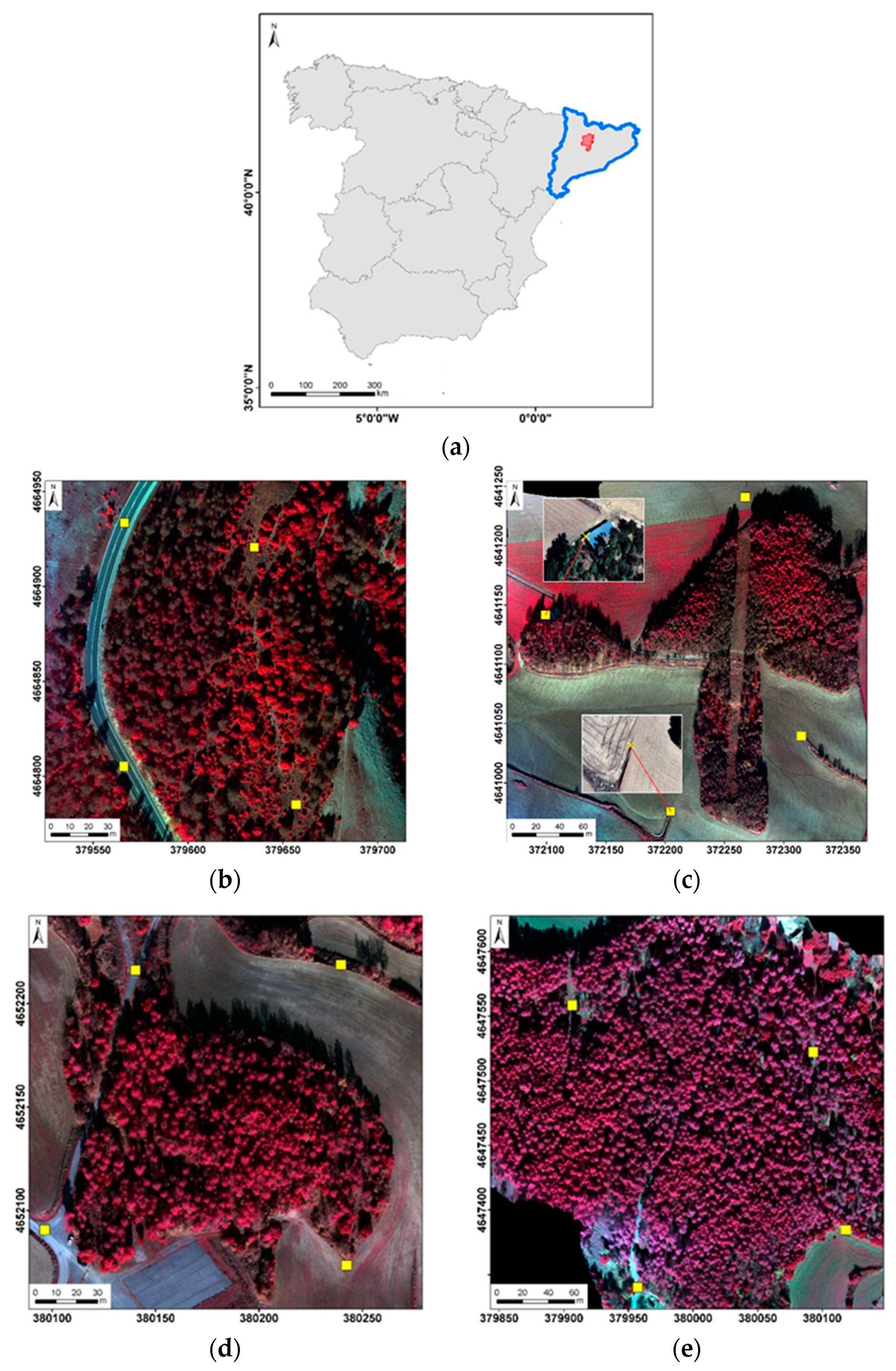
The study was conducted in four pine-dominant stands, including Codo, Hostal, Bosquet, and Olius in the region of Solsona, Catalonia, Spain (Figure 1a), covering 64 hectares in total where the recent expansion of T. pityocampa has been recorded in the regional forest health inventory (Generalitat de Catalunya). They represent a Mediterranean continental climate with hot dry summers and mild wet winters at elevations ranging from 600 m to 1300 m. According to the Land Cover Map of Catalonia (MCSC) for 2009, forest stands were typically dominated by Pinus nigra and P. sylvestris, which are often mixed with evergreen oak species such as Quercus ilex.
2.2. UAS Image Acquisition and Processing
In this study, a quadcopter (Phantom 3, DJI) was used as an UAS platform, equipped with a high spatial resolution multispectral camera (SEQUOIA, Parrot) carrying a payload of 72 g, to capture both visible RGB and invisible NIR images simultaneously. The RGB camera has a resolution of 16 megapixel with a lens focal length of 5 mm and fields of view (FOV) with horizontal (HFOV): 63.9°, vertical (VFOV): 50.1°, and diagonal (DFOV): 73.5°. In addition, another 1.2 megapixel sensor, with a lens focal length of 4 mm, and fields of view with HFOV: 61.9°, VFOV: 48.5°, and DFOV: 73.7°, captures four spectral bands in green (530–570 nm wavelength), red (640–680 nm wavelength), red edge (730–740 nm wavelength), and near infrared (770–810 nm wavelength). Both RGB and NIR images were collected simultaneously from a flying altitude at 76–95 m above the ground level with 80% forward and side overlap at speeds ranging from 4–8 per second, achieving a ground sample distance of 2.0 cm with the RGB camera and 7.4 cm with the NIR camera, on average. Four flights were conducted in winter 2017–2018 on clear sunny days around noon to minimize the effects of clouds and shadows, covering the total area of 64 hectares. The flight features with the RGB and NIR cameras were summarized in Table 1.
A total of 1042 adjacent photos, overlapped from the flights with their geotagged locations, were processed separately for those captured with the RGB and NIR cameras in the software, PhotoScan Professional 1.4.0 (Agisoft LLC, St. Petersburg, Russia). In image processing, the photos were geometrically aligned to build a point cloud, 3D model, digital elevation model (DEM), and digital surface model (DSM). For generating orthomosaic images, those composed of multispectral bands were radiometrically corrected to calibrate the reflectance values corresponding to each band, by using reflectance panels which were captured before each flight specific to the lighting conditions of the date, time, and location of the flight [38,39]. The use of a reflectance panel captured as an image of calibrating a white balance card enabled the PhotoScan to recognize the images’ reflectance according to known values of all spectral bands written on the panel for radiometric calibration [38]. Using the ArcGIS version 10.5 software (ESRI, Redlands, CA, USA), each orthomosaic was georeferenced to the 1:2500 orthophotos [40] in the cartographic UTM projection by performing a first order polynomial transformation with four ground control points (GCPs) of clearly visible features such as roads, structures, and field edges across each study area (Figure 1b–e), obtaining an accuracy of sub-meter root mean square error (RMS). As alternative ground validation data, we used the UAS orthomosaic images and DSM captured at a very higher spatial resolution (2.0 cm) with the RGB camera.
2.3. Vegetation Indices
Given the four bands in NIR imagery obtained from UAS flights, we calculated vegetation indices (VIs) which may extract the relevant information on different vegetation features for further analysis. The chlorophyll absorption is very high in the visible spectrum, where the reflectance is the highest for green wavelengths [17]. In shifting from the range of visible wavelengths to invisible towards the NIR, the reflectance starts to increase for red edge wavelengths as the chlorophyll absorption ceases [17]. For automated classification and repeated application, four normalized VIs based on various combinations of spectral bands were selected as comparable thresholding values among the four different study areas (Table 2). NDVI has been most commonly used for detecting land cover change and mapping forest defoliation due to its sensitivity to low chlorophyll concentrations [17,41]. On the contrary, green NDVI (GNDVI) is sensitive to high chlorophyll concentrations and accurate for assessing chlorophyll content at the tree crown level [41]. By exploring various combinations of available spectral bands, we additionally examined the sensitivity of other indices such as green–red NDVI (GRNDVI) and NDVI red edge (NDVIRE) to find the most sensitive VI to classify forest defoliation and tree species.
2.4. Pixel-Based Thresholding Analysis
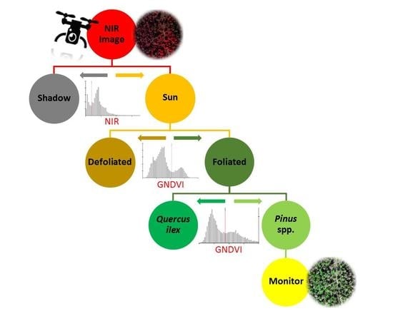
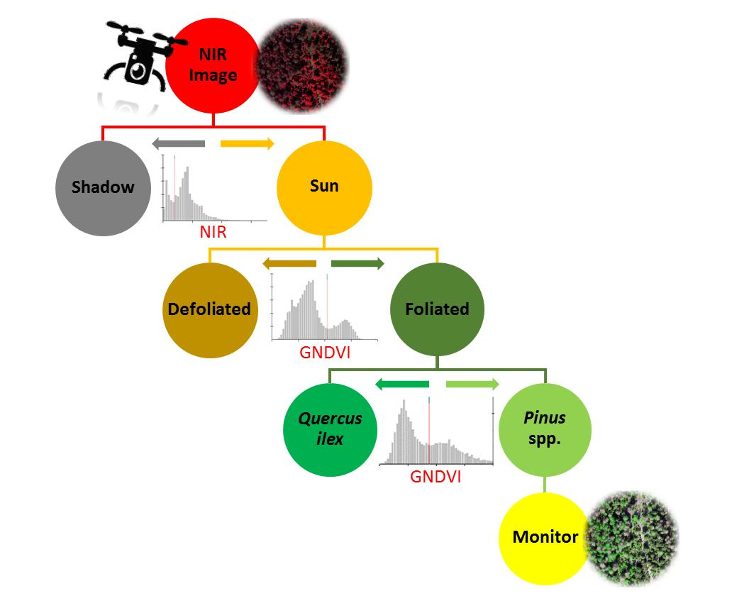
In this study, histogram thresholding analyses, known as the classical approach to classification [27,29,45], were explored in a nested method for excluding shadow from sun pixels, detecting defoliation from foliated green pixels, and discriminating pine from evergreen oak. Using the ArcGIS version 10.5 software, available spectral bands and Vis from the UAS-derived NIR imagery were analyzed in a histogram distribution by the first valley detection thresholding with local minima. Figure 2 simplifies a workflow of the nested histogram thresholding analyses per study area, from the initial shadow removal with the NIR band to the final separation of pixels by defoliation and tree species for monitoring, so that this method can be repeated to conduct a time series image analysis.
2.4.1. Shadow Removal
Although all flights were conducted around noon when the sun angle is considered to be minimum to generate shadows in images, there are often some limitations to achieving shadow-free images. Among several shadow detection algorithms suggested and compared by Adeline et al. [29], a histogram thresholding analysis performed well as the most robust method and demonstrated good results with an NIR band alone. Generally, the location of shadows in the histogram should be separated at the first valley of multimodal distribution with two or more peaks [12,28,29]. We then applied the method, first valley detection thresholding, using the UAS-derived NIR band to exclude shadow pixels from further analysis to reduce uncertainty.
2.4.2. Defoliation Detection
Following shadow removal, shadow-free pixels in each study area were extracted by a mask of pine-dominated forest polygons mapped on the MCSC. The same histogram thresholding approach was applied to separate the masked pixels representing green tree crown from non-green in each study area with four VIs (Table 2). In this analysis, green pixels with leaves were defined as foliated class, while non-green pixels without leaves belonged to the defoliated class. While the previous study in the Codo area [16] applied pixel-based unsupervised classification with NDVI to calculate the percentage of defoliation per tree crown area identified by individual tree delineation algorithm, in this study we simply focused on determining the threshold values of four VIs and their variations among four study areas as well as evaluating the performance of each VI.
2.4.3. Foliated Species Discrimination
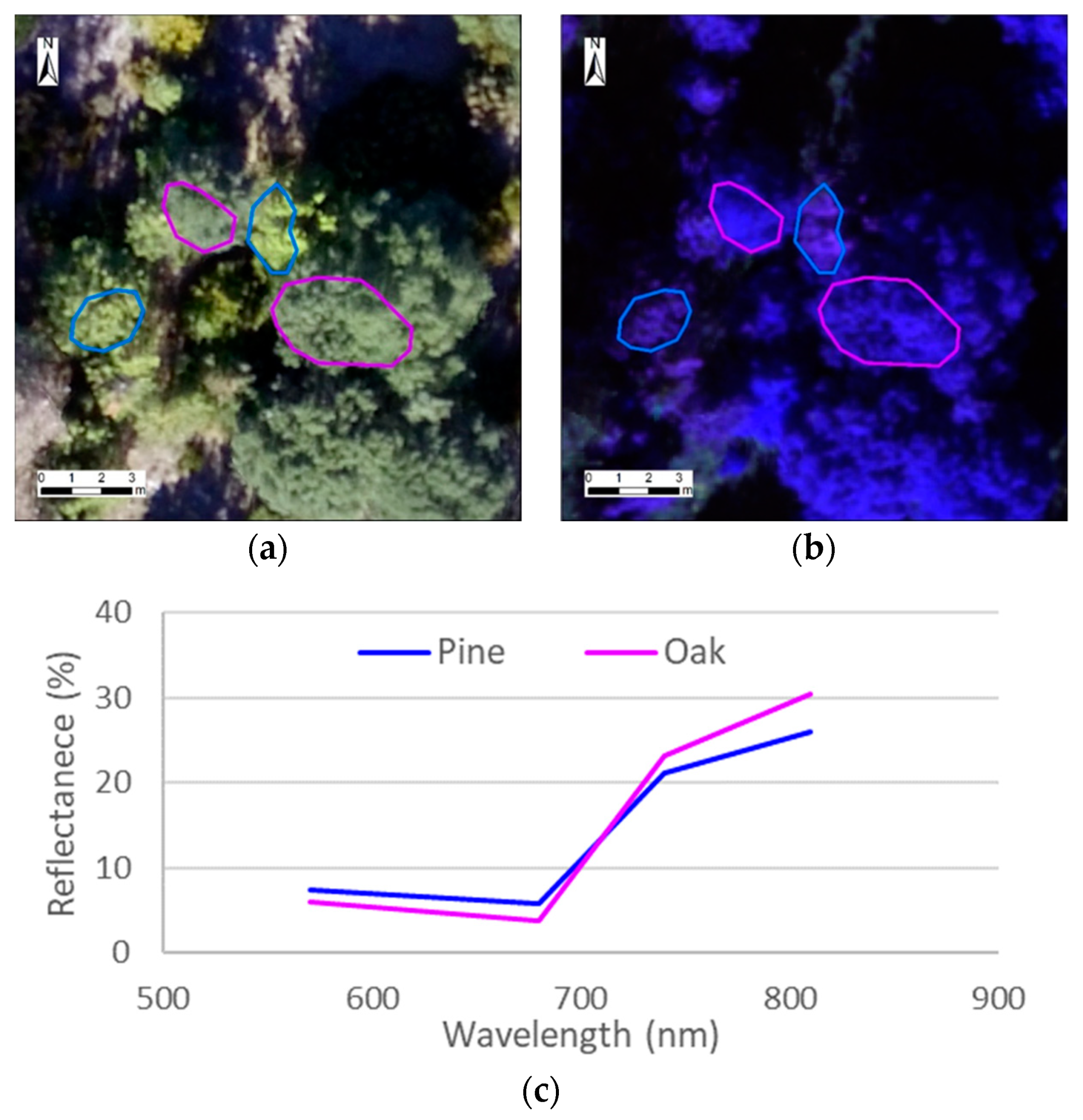
To distinguish shadow-free foliated trees of pine species from evergreen oak, we first visually interpreted RGB images. Once 10 pines and 10 evergreen oaks in each of two study areas (Codo and Olius) were manually selected in RGB orthomosaic images (Figure 3a) and delineated to extract sample pixels based on NIR imagery representing each species (Figure 3b), histogram thresholding analyses were applied to those selected pixels showing the spectral profiles in Figure 3c. Relatively, the color intensity and texture of pine species are softer than evergreen oak species [46]. Moreover, broadleaf vegetation reflects notably higher values of NIR than needle-leaf vegetation [47] as observed in our study area with spectral profiles of the two species for the wavelength range of 770–810 nm (Figure 3c). However, the previous study in the Codo area [16] suggested that NIR alone or standard NDVI [42] may not be sufficient to distinguish two species by thresholding analysis. Thus, for further exploring species discrimination, we applied the histogram thresholding method with the three additional VIs (Table 2) to pixels extracted by sample crown polygons. There were only a few evergreen oak samples observed in the other two study areas (Hostal and Bosquet), which were not included in this analysis.
2.5. Object-Based Random Forest
In contrast to determining threshold values for pixel-based classification, we used another method, object-based Random Forest, with the advantage of analyzing combined data of multiple spectral bands, spatial parameters, and textural properties. As shown in Figure 4a, color infrared (CIR) images composed of NIR, red, and green bands were first computed for automatically aggregating adjacent pixels that are similar in spectral properties as image segments (Figure 4b) in the ArcGIS version 10.5 software. To supervise Random Forest classification, sample data were then trained as segments of shadow, defoliation, and tree species such as pine and evergreen oak, which were comparable to the thresholding analysis in Codo and Olius study areas. CIR images may contain more effective parameters as predictive indices characterized by relative color, color intensity, and texture [46].
2.6. Validation and Accuracy Assessment
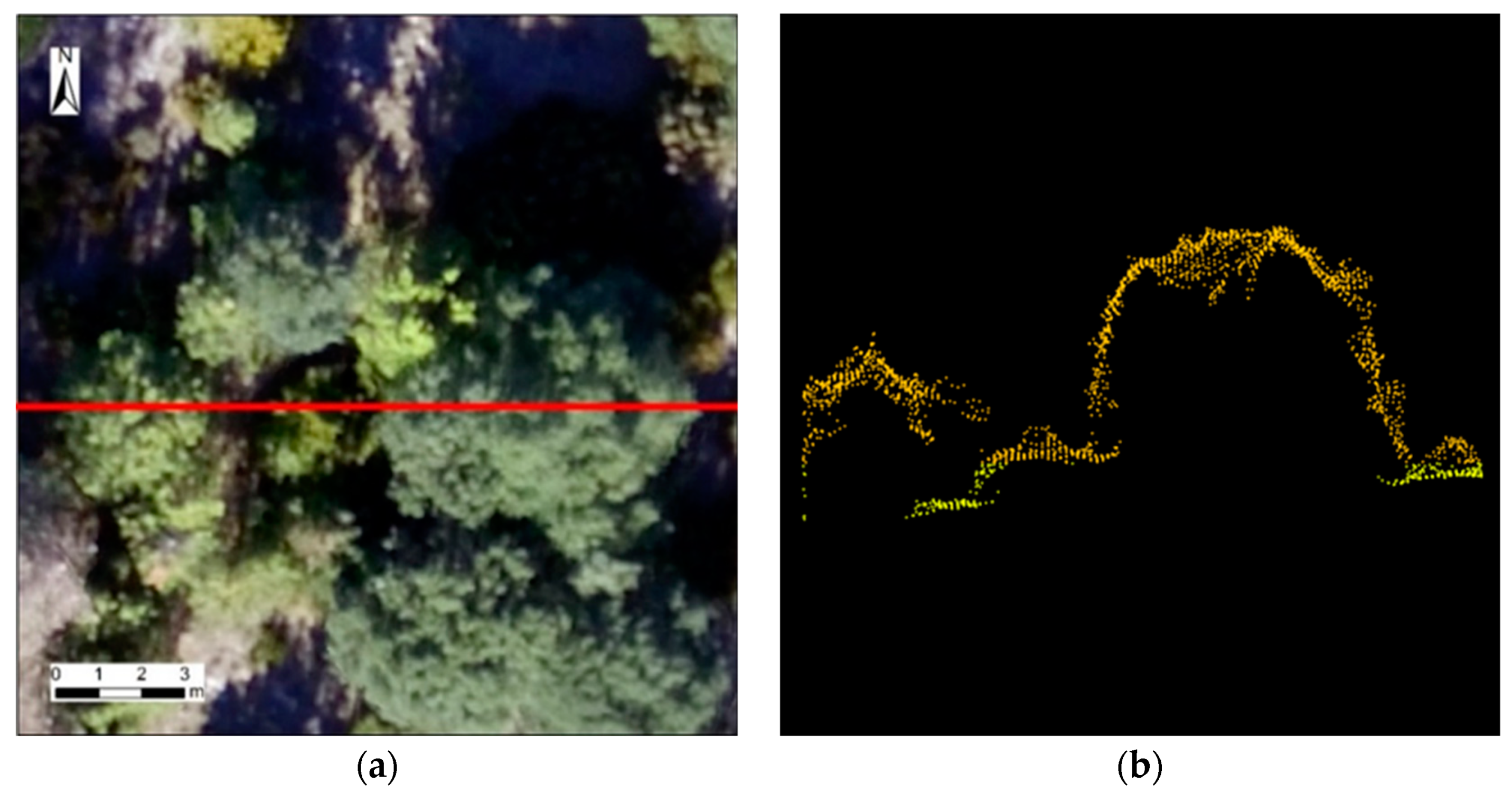
Ground validation data were obtained by photointerpretation of the RGB orthomosaic images (Figure 5a) and DSM (Figure 5b), at a very high spatial resolution (2.0 cm), which was higher than the resolution of NIR imagery (7.2 cm) based on the separate multispectral camera from the same UAS flight. The DSM profile, in particular, enabled to generate a 3D stand structure and distinguish soils from defoliated tree branches, which might have been misinterpreted due to the similar colors in the RGB orthomosaic images. We then observed plots of the RGB images classified as: (1) shadow or sun pixels, (2) defoliated or foliated for the sun pixels, and (3) pine or evergreen oak species for the foliated pixels. Such validation by photointerpretation has been increasingly used as an alternative to conventional ground truth data in recent studies with promising results [15,16,48,49,50].
In each study area 100 pixels were randomly selected to assess the accuracy of final classification results by histogram thresholding analyses and Random Forest, separately, with predicted indices derived from the NIR imagery, in reference to ground observations based on the RGB orthomosaic images. A confusion matrix was then generated to compare producer’s and user’s accuracy indicating omission and commission errors, respectively, as well as overall accuracy. To explore the uncertainty in the best performed results over the total study area, the overall accuracies were further investigated in a sensitivity analysis, testing the robustness of the estimated thresholds by increasing and decreasing values.
3. Results
3.1. Pixel-Based Thresholding Analysis
3.1.1. Shadow Removal
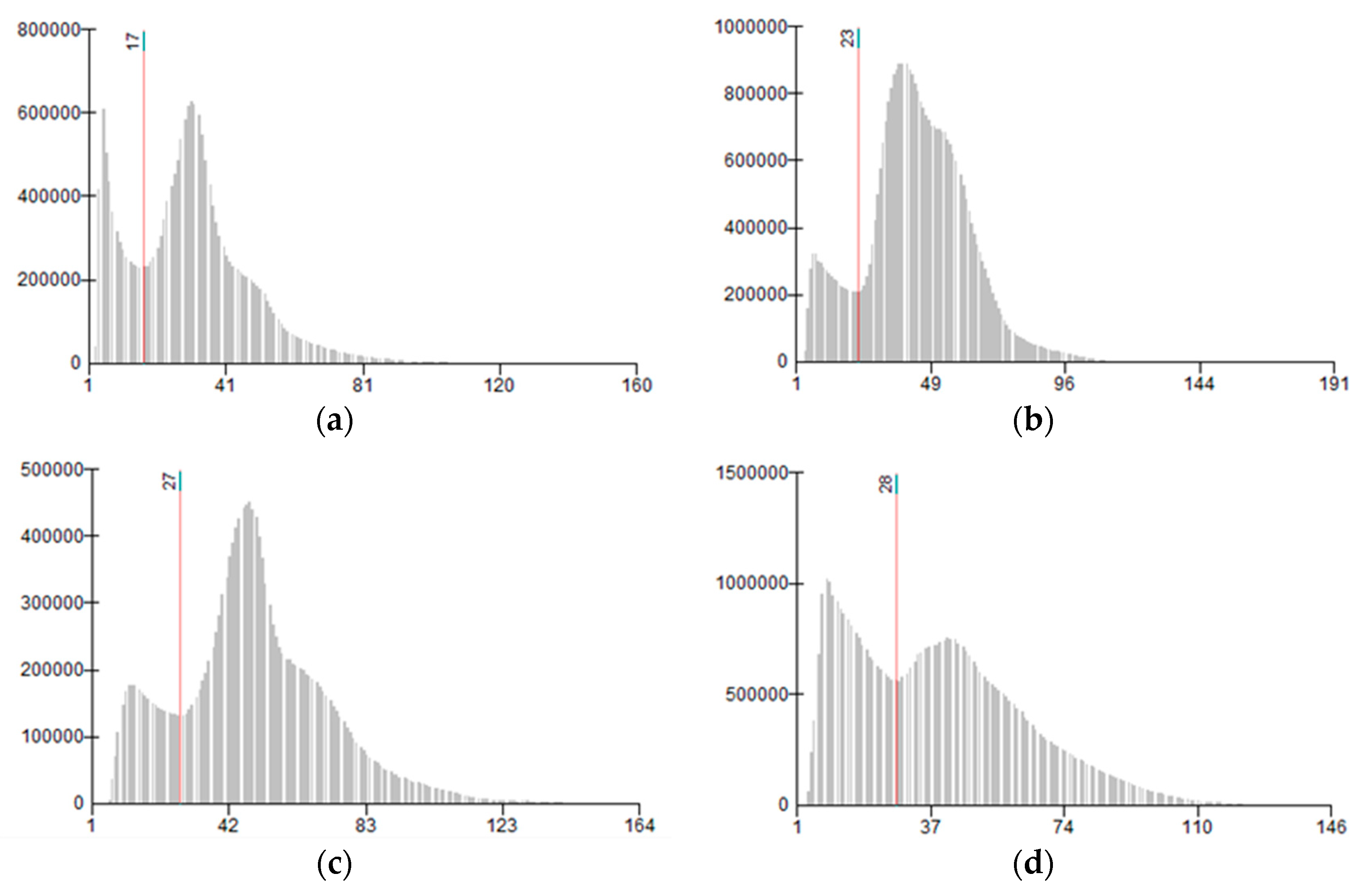
A multimodal histogram distribution of NIR values was shown by study area in Figure 6, with the first valley determined as the thresholding value to exclude shadow pixels indicating the lowest class of reflectance in the NIR band. As shown in Figure 6a for the Codo area, those pixels with a value smaller than 17 were classified as shadow areas, accounting for 29% of the total number of pixels, thus excluded to reduce uncertainly. Likewise, shadow areas resulted in 14% for Hostal (Figure 6b), 17% for Bosquet (Figure 6c), and 35% for Olius (Figure 6d) study areas. We found a variation in the threshold values among the four study areas compared in Table 3, ranging from 17–28.
3.1.2. Defoliation Detection
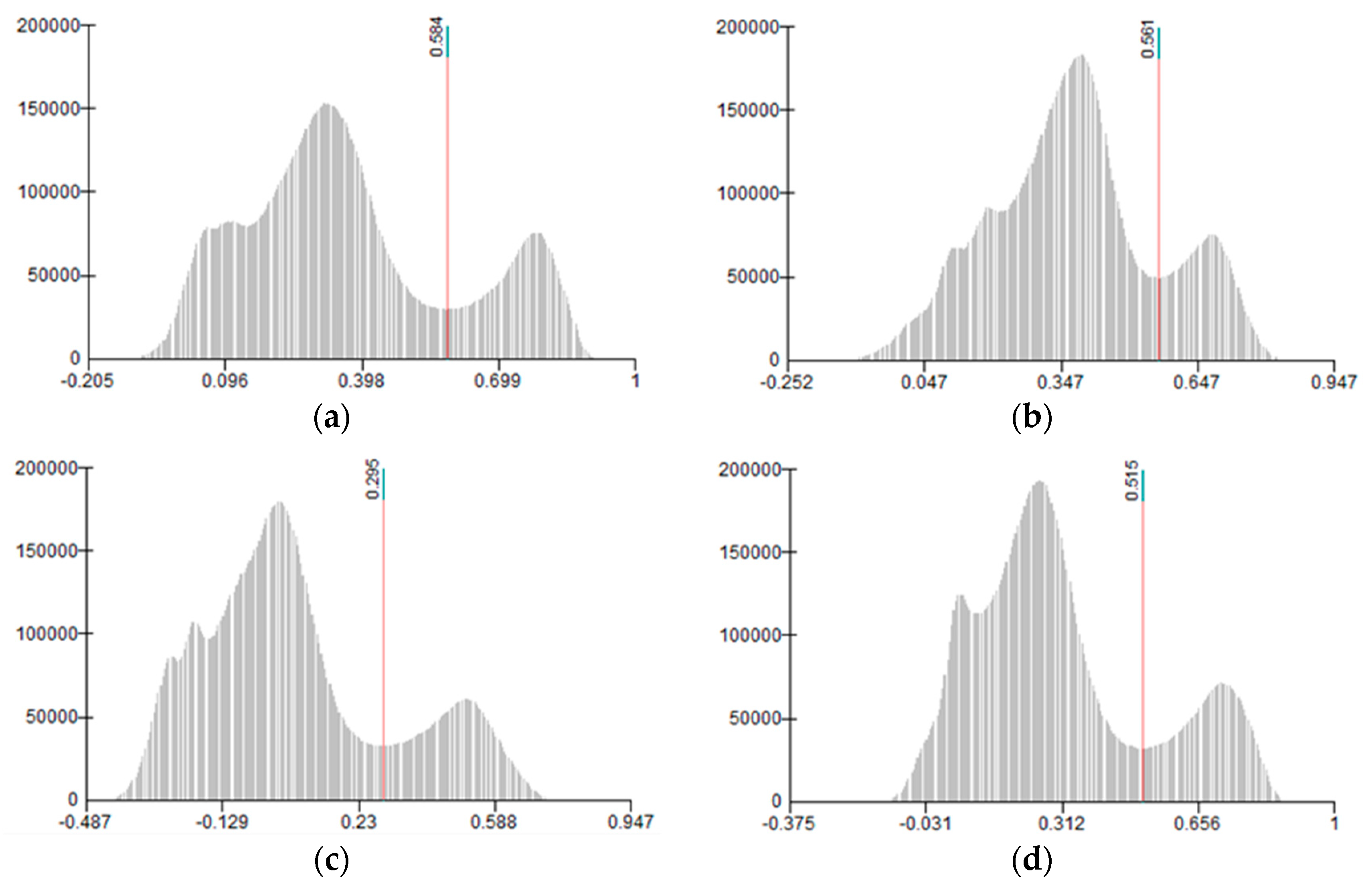
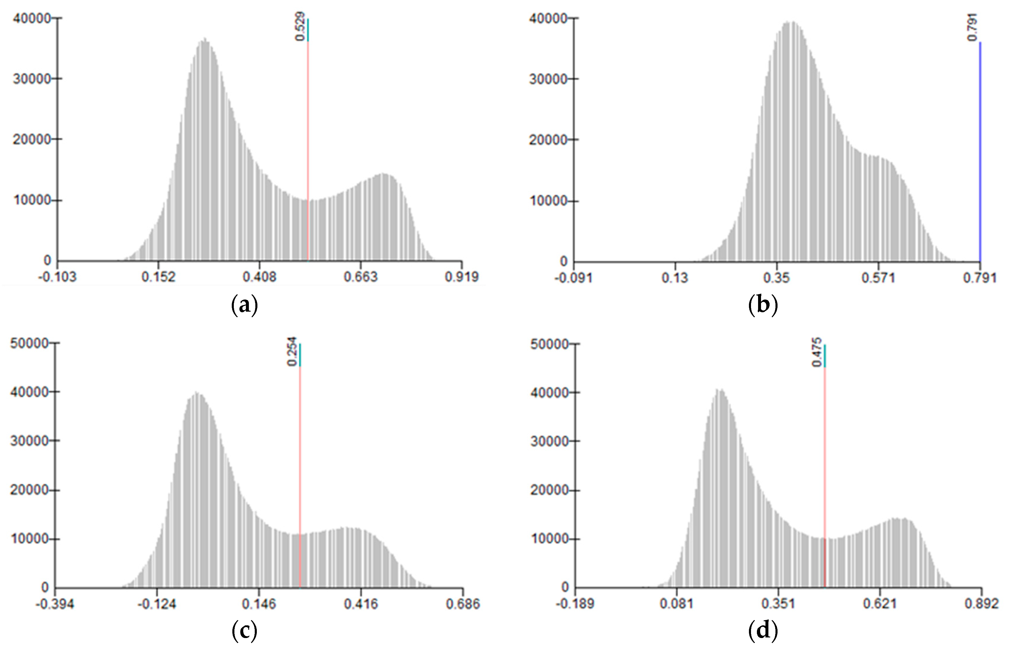
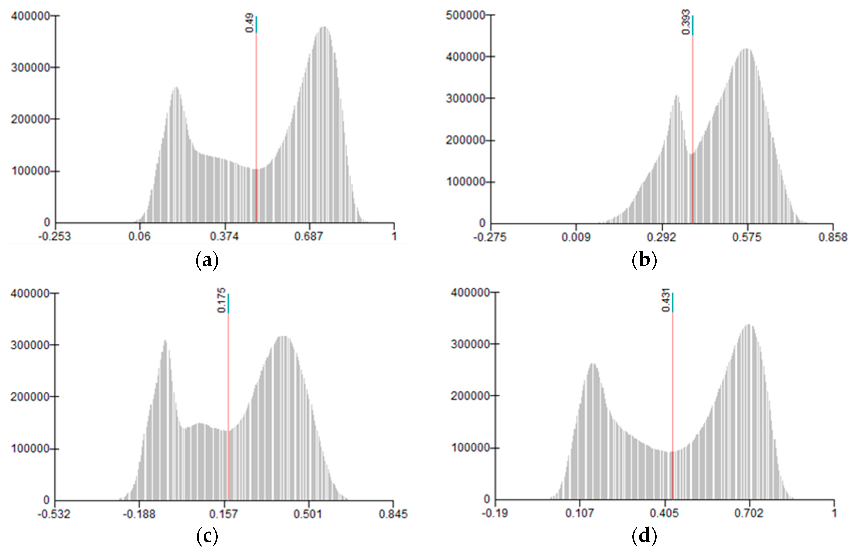
Each histogram distribution of pixel values calculated for NDVI, GNDVI, GRNDVI, and NDVIRE was presented in Figure 7 for the Codo study area. The final valley of multimodal distribution determined the threshold value to separate the highest class of reflection in each index classified as foliated to mask green tree crown pixels. All threshold values determined by the same method in the other three study areas (Figure A1, Figure A2 and Figure A3) are summarized in Table 3, with a various range of NDVI (0.481–0.584), GNDVI (0.393–0.561), GRNDVI (0.171–0.295), and NDVIRE (0.416–0.515) including the average values. We found some exceptions for those unimodal distributions with no valley detected with GNDVI in Hostal (Figure A1b) and Bosquet (Figure A2b).
3.1.3. Foliated Species Discrimination
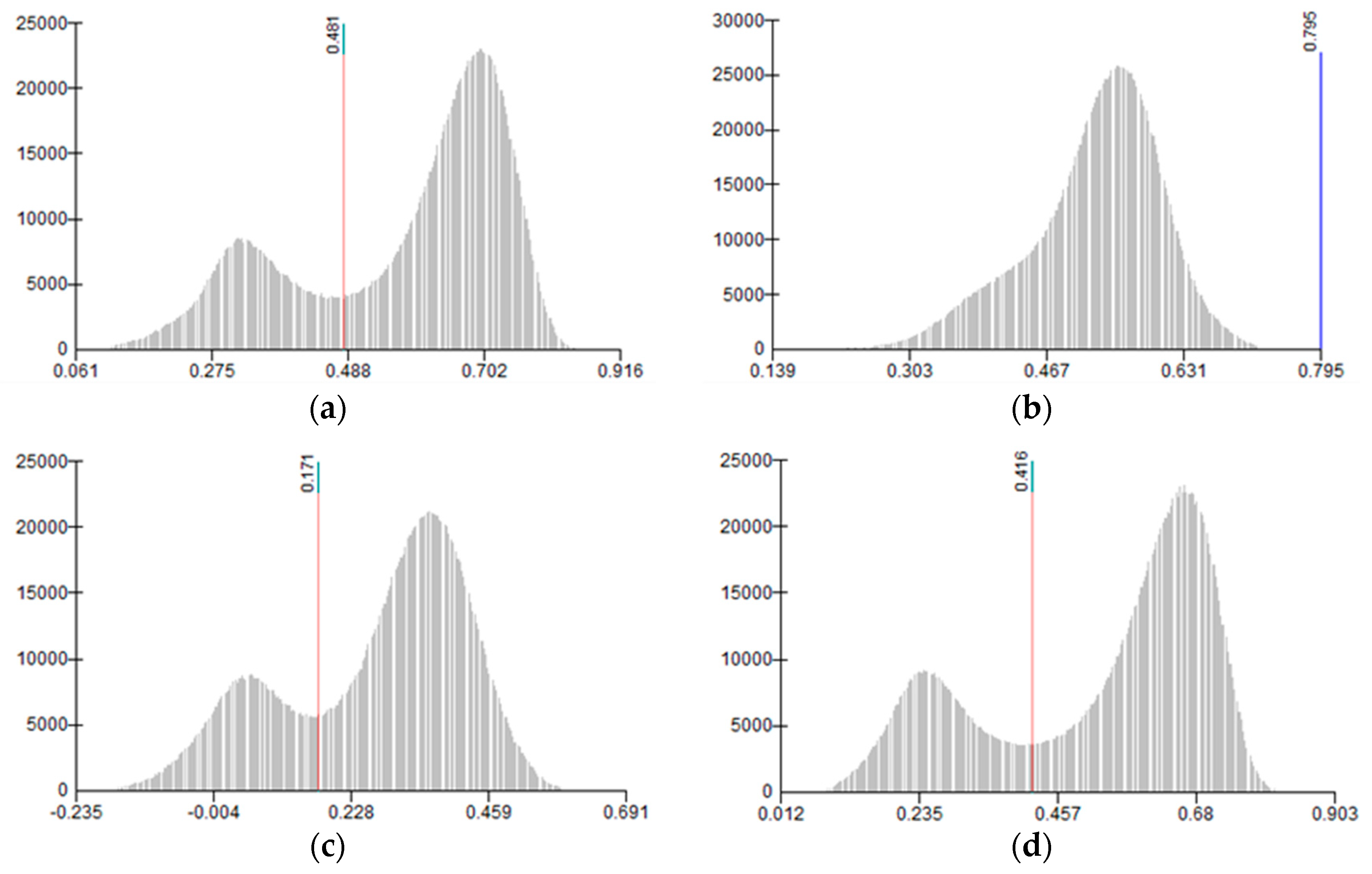
For discriminating species between pine and evergreen oak in Codo and Olius study areas, shadow-free foliated pixels were classified as shown in Figure 8. Among the four VIs analyzed, GNDVI and GRNDVI resulted in a bimodal distribution in Codo (Figure 8b,c), revealing two distinguishable species classes between pine and evergreen oak, while the rest of our results with NDVI (Figure 8a) and NDVIRE (Figure 8d) did not achieve this distinction. The first valley of bimodal distribution, indicating the lower class of reflectance in each index, was classified as pine to mask host tree species. In Olius, on the other hand, only the histogram with GNDVI showed a bimodal distribution (Figure A4b). However, we found that the threshold value of GNDVI for separating pine from evergreen oak in Codo (0.681) was notably close to the one (0.631) in Olius, as summarized in Table 3.
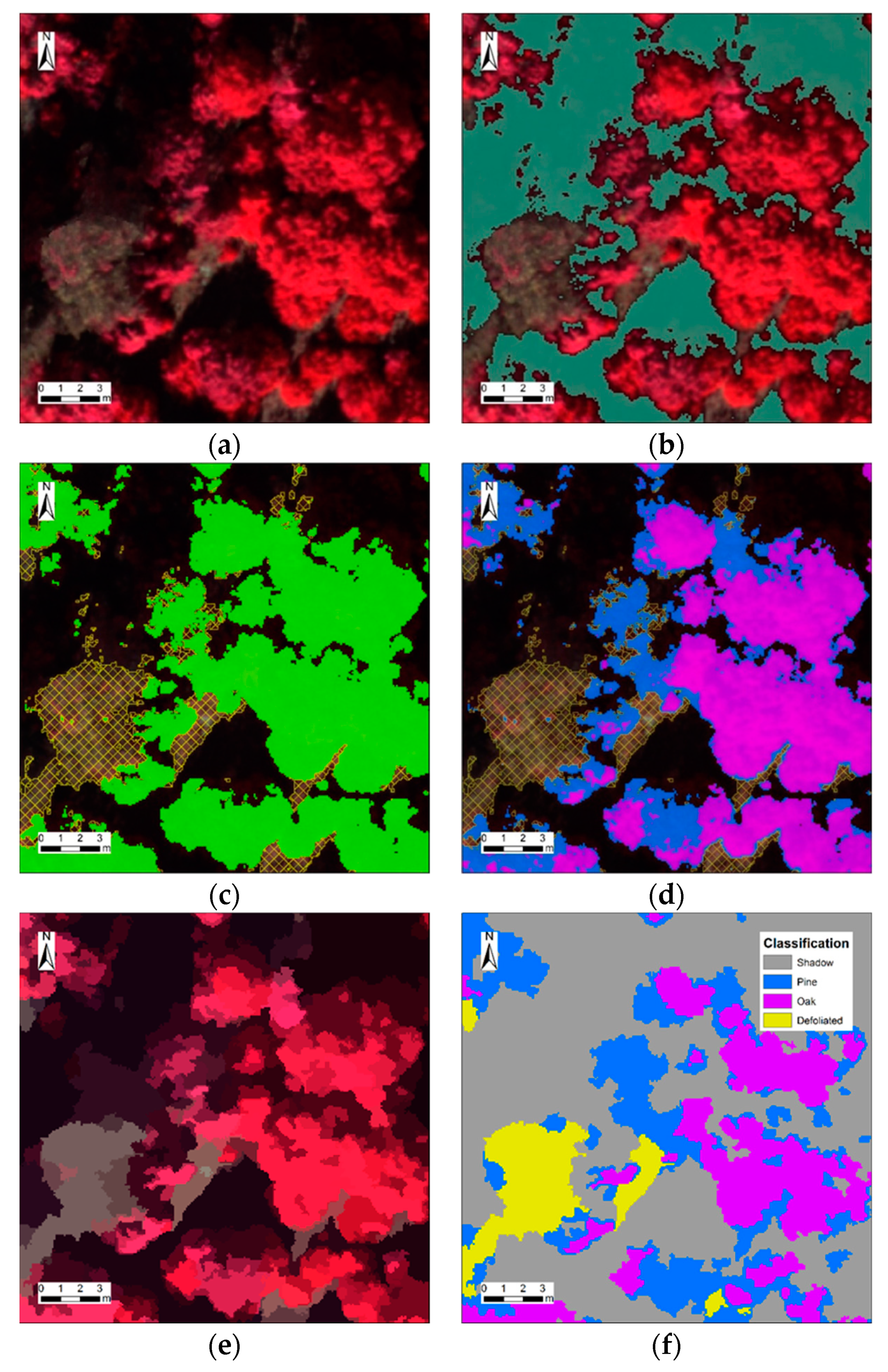
The above results of histogram thresholding analysis are illustrated in Figure 9, starting with a CIR image (Figure 9a) overlaid with NIR highlighting shadow pixels in gray (Figure 9b). Following shadow removal, the CIR image was overlaid with GNDVI highlighting shadow-free defoliated pixels in meshed yellow and foliated pixels in green (Figure 9c), which were further classified and highlighted as pine in blue and evergreen oak in purple (Figure 9d).
3.2. Object-Based Random Forest
As shown in Figure 9e, image segmentation enabled the aggregation of adjacent pixels with similar spectral properties in CIR imagery (Figure 9a). Following training sample segments with supervised Random Forest classification, the resultant segments were classified into shadow, defoliated, pine, and evergreen oak (Figure 9f) in comparison to the results of thresholding classification (Figure 9d).
3.3. Validation and Accuracy Assessment
Classes defined by histogram thresholding analyses (Table 4, Table 5, Table 6 and Table 7) and Random Forest (Table 8 and Table 9) were validated by a confusion matrix evaluating shadow, defoliation, and species with referenced RGB images and DSM as ground observations. The confusion matrix for classifying shadow and sun is detailed in Table 4 based on totaling 400 randomly selected pixels, showing that the higher producer’s accuracy was 96% for the sun class where 212 out of the 220 pixels observed as sun were correctly classified by predicted NIR, while the shadow class showed a higher user’s accuracy of 95% where 167 out of the 175 pixels predicted as shadow correctly represented the observed class. To analyze any variation among all study areas, overall accuracies were calculated by each area to compare the performance to the one totaled in Table 5, resulting in a total overall accuracy of 95% without any significant discrepancy by study area.
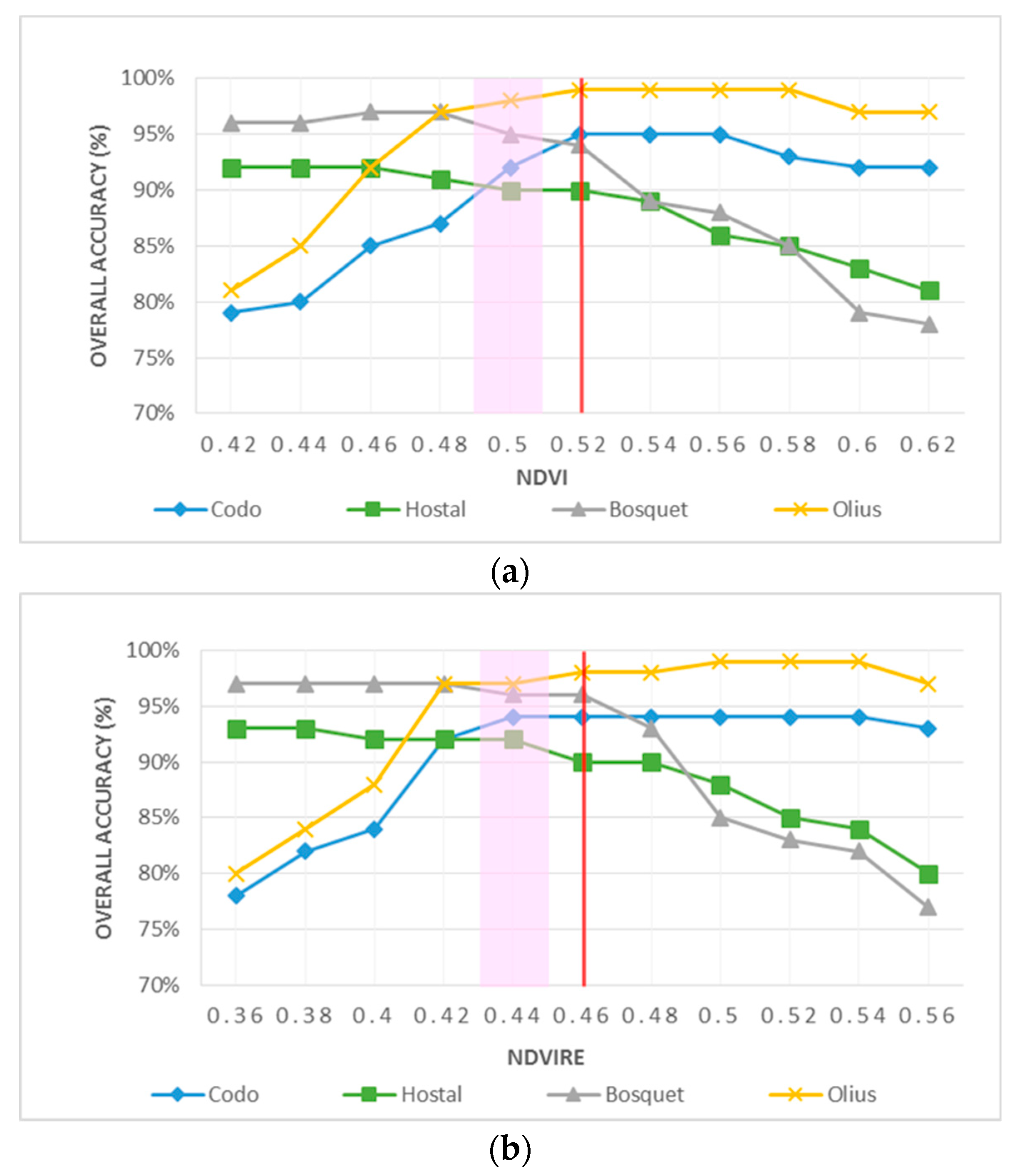
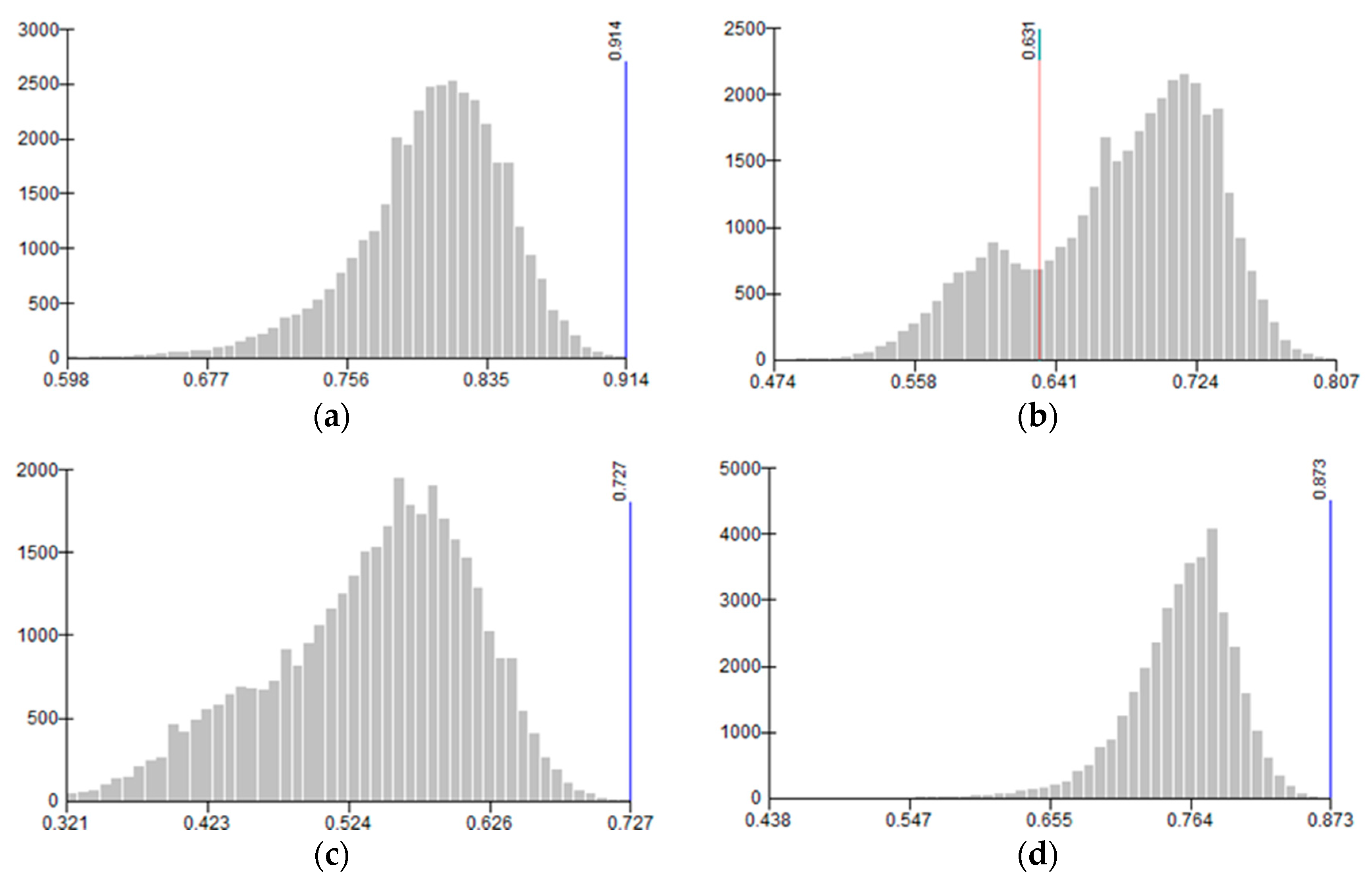
For classifying defoliated and foliated pixels, overall accuracies were assessed in the same manner and compared among the four predicted VIs in the four study areas (Table 6). When the total overall accuracy based on totaling 400 randomly selected pixels was calculated per study area, NDVI and NDVIRE equally performed the best with a total overall accuracy of 95%, followed by GRNDVI with 92%, while it was not evaluable with GNDVI due to undetermined threshold values in Hostal and Bosquet. Since we were also able to estimate the average thresholds of best performed NDVI and NDVIRE over the total study area, the accuracy assessment was complemented with a sensitivity analysis, shifting the average threshold values by 0.02–0.1. As shown in Figure 10a,b, the optimal threshold values (0.50 for NDVI and 0.44 for NDVIRE), where the difference in overall accuracies is the smallest across the four study areas, were highlighted resulting in slightly lower values than the estimated average.
For evaluating the accuracy of species discrimination, we conducted a third confusion matrix in the same manner by assessing overall accuracies with GNDVI in each of two study areas, Codo and Olius, as shown in Table 7. With an overall accuracy of 96%, GNDVI performed better in Codo study area than in Olius (93%). After visual inspection, we found that most errors derived from those randomly selected pixels that occurred to be near the boundary area between two classes.
Finally, Table 8 and Table 9 by study area show the integrated confusion matrix of object-based Random Forest, which enabled to segment CIR images composed of three spectral bands and distinguish four classes of shadow, defoliated, pine, and evergreen oak at the same time with overall accuracies of 93% in Codo and 91% in Olius, as high as those results combined from Table 5, Table 6 and Table 7.
4. Discussion
Our methodology explored the capabilities of UAS-derived high spatial resolution NIR imagery for monitoring forest defoliation caused by T. pityocampa in small pine-dominated stands mixed with evergreen oak. Using a simple histogram thresholding analysis as a classification technique, the overall results showed that specific spectral bands or NIR-derived VIs perform better than the others for discriminating shadow, defoliation, and foliated tree species, which was determined by accuracy assessment in a confusion matrix. In contrast to this simple classification approach, we also used a more complex and robust object-based image classification technique with Random Forest, resulting in overall excellent performance as expected from the literature reviews [33,34,35,36,37].
4.1. Shadow Removal
Shadow detection using a histogram thresholding analysis with an NIR band has been explored in several studies on forest areas following urban and agricultural areas [29,31,45,51]. One of the disadvantages of this technique is that it can often be difficult to distinguish shadow areas and other dark surfaces such as water bodies [45]; however, this limitation did not apply to our small study areas where no water features such as river, lake, or ocean were found. Miura and Midorikawa [52] classified shadow areas by a histogram thresholding analysis using the NIR band from IKONOS data in order to eliminate shadow pixels that were difficult to accurately detect slope failure based on the difference in NDVI between the pre- and post-earthquake images. Lu [53] also separated vegetation from shadows with the thresholds based on the IKONOS NDVI or NIR images, although it was difficult to extract cloud shadows from tree shadows. Martinuzzi et al. [54] developed a method for detecting shadow areas in the NIR band from Landsat data to mask cloud shadows, including topographic shadows which were not successfully discriminated from each other. This type of limitation to separating topographic shadows from cloud shadows is not an issue in the UAS imagery as flights can be conducted under clouds.
Although in our study shadow areas were eliminated with high overall accuracies, those may be corrected by supervised classification training samples for different shadowed land cover types, instead of excluding them from further analysis. Other types of shadow corrections include deshadowing by scaling shadow pixels with combined spectral criteria of NIR and shortwave infrared bands derived from satellite images [55], which are more sensitive to shadow effects than visible bands, while a combination of RGB and NIR bands captured by airborne cameras was explored for diffusing shadow effects and validated by field measurements with a good agreement [56]. Thus, shadow correction methods should be explored for our further studies by developing a tool to combine spectral criteria from available bands and/or conducting extra flights within the following days or weeks over the same area of interest around the same time of the day to be comparable among them.
4.2. Defoliation Detection
Focusing on forestry applications over the past decade, NDVI derived from UAS has been increasingly used for detecting defoliation at high spatial resolutions and assessing damage severity by classification techniques [10,12,14,15,16,23,24,25]. A continuous improvement in overall accuracy was demonstrated in our study by using histogram thresholding classification with the four VIs. NDVI and NDVIRE performed the best with an overall accuracy of 95%, followed by GRNDVI with 92% while GNDVI was excluded due to poor performance in determining the threshold values, which may be explained by the difference in reflectance between two bands selected for calculating each index. We could explain that the reflectance is generally higher in the green band due to chlorophyll absorption in blue and red bands [17,47]. Another explanation could be that unhealthy leaves show a notably higher reflectance than healthy leaves in the range of RGB visible light due to a decrease in chlorophyll content, while healthy leaves show significantly increased and exceeding reflectance in both the red edge and NIR bands [15,57,58]. Therefore, a larger difference in reflectance between the two bands used in any formula (Table 2) leads to higher index values and indicates healthier leaves. At least for the forest types analyzed in our study, there was no significant difference between NDVI and NDVIRE. In other words, the red edge band was not particularly more sensitive to defoliation than the NIR band.
Opportunities for future improvements include defoliation detection at the pixel level in integration with the UAS-derived canopy height model (CHM) at the 3D tree level to automatically delineate individual tree crowns and extract only pixels detected by the height of interest [14,16,48]. For monitoring the forest inventory as a function of ecosystem services, it will be necessary to estimate the overall defoliation degree per individual tree which can be calculated by the ratio between pixels grouped as defoliated and foliated per tree [16]. For further 3D tree research, detecting the structural change of defoliated trees may be explored as an additional parameter by quantifying a dense point cloud [15,59,60,61,62], which may contain information on cumulative defoliation in time series imagery, where the density of points on defoliating trees may start to decrease over time [62].
4.3. Foliated Species Discrimination
As the UAS technology advances, studies on species discrimination for forestry applications [24,63,64,65] have increased using various classification methods. Most recently, Cardil et al. [16] applied thresholding classification with NDVI to distinguish among Pinus spp. with three levels of defoliation and from Quercus ilex in Codo, Spain, with an overall accuracy of 81%. The classification accuracy was re–evaluated in two of our study areas where we distinguished foliated Pinus spp. from Q. ilex by histogram thresholding classification with GNDVI with an increased overall accuracy of 93–96%. We again demonstrated that this comparison among various VIs led to improve the classification results on species discrimination with GNDVI showing a bimodal histogram distribution in both the two study areas. This may suggest that the relation between green and NIR bands is the key measure to distinguish broad leaves from needle leaves among healthy trees, while GNDVI showed poor performance in defoliation detection. Several studies have suggested that the use of green bands in NDVI is more sensitive to chlorophyll which is well correlated to leaf area index [41,43,66] as well as that broad leaves show a much higher reflection in the NIR range than needle leaves [47,67,68]. To examine the robustness of GNDVI for species discrimination, the similar threshold values determined in Codo and Olius should be reapplied to additional pine–oak mixed stands in new study areas.
It should be noted that UAS imagery has the advantage of separating pine trees from other species in mixed stands at tree level, enabling the exclusion of non-pine pixels for further analysis, while this may not be capable with Sentinel-2 [18] or Landsat 8 [69] data at medium spatial resolutions (10–30 m), which are too coarse to assess an individual tree crown area. Although the enhancement at spatial and temporal resolution is one of the significant advantages for using UAS imagery, the spectral resolution by Parrot SEQUOIA is limited to capturing RGB, red edge, and NIR bands, with wider bandwidths in the wavelength in comparison to other airborne sensors and satellites which are required to detect more features with narrower and/or specific bandwidths. Nonetheless, the Parrot SEQUOIA has been widely used for a relatively good economic performance trade-off in operational forestry and agriculture applications, with the additional advantage of applying such high-resolution data to calibrate medium-resolution satellite data [39,49,50,70].
4.4. Classification Techniques
General findings in the above-mentioned studies suggest that the overall accuracy for shadow removal, defoliation detection, and species discrimination should increase as the number of classes decreases, regardless of the technique used for classification. As observed in our study, a series of pixel-based thresholding analyses generated slightly higher overall accuracies in each confusion matrix for predicting two classes than object-based Random Forest for predicting four classes in one combined confusion matrix. One of the limitations of histogram thresholding analyses is that spatially isolated and fragmented pixels (Figure 9b–d) were as small as a ground resolution of approximately 7 cm to identify the class and assess the accuracy against the referenced orthomosaic image, unless pixels with similar digital number (DN) values were aggregated. To restrict pixels at a very high spatial resolution from being dispersed, object-based classification techniques enable to merge them with adjacent segments according to certain minimum segment size or shape [33]. Despite these limitations, our study highlighted the simplicity of the histogram thresholding method to suggest combining the best indices for a series of classifications to extract the relevant information on different vegetation features.
4.5. Future Research Directions
Among four study areas defined as pine–dominated by land cover map, we noted that all threshold values of VIs in Codo study area for detecting defoliation were relatively higher than those in the other three study areas (Table 3). This may be explained by the seasonal difference in reflectance since the UAS imagery in Codo was captured in the end of November 2017, which was almost two months before the rest of the UAS flights were conducted in January 2018. It should also be noted that in Hostal study area the valley detection thresholding to separate foliated class in the multimodal distribution with GRNDVI (Figure A1c) was not as clear as those with NDVI (Figure A1a) or NDVIRE (Figure A1d), which is one of the disadvantages of histogram thresholding analyses [29,31]. Consequently, due to this ambiguous discrimination between defoliated and foliated classes, the classification accuracy with GRNDVI in Hostal turned out to be 84%, notably the lowest among the four study areas and VIs tested. As a solution to mitigate any potential errors, multiple flights over the same study area should be repeated at different dates to determine whether each threshold value is specific to a study area and/or season for accuracy improvement and monitoring purposes. Provided that the variation in the threshold limits among our study areas may have been affected by different flight dates, weather conditions, stand structures, and species composition which are not distinguishable by land cover map, the estimated average limits in Table 3 are not yet well established to be directly applied to new study areas on a large scale. Whether the similarity in the range of threshold limits can be achieved in similar forest types should be explored by applying the average or optimal threshold values (Figure 10a,b) to additional study areas.
Nevertheless, the enhanced UAS technology enabled us to achieve flights with both RGB and NIR multispectral cameras simultaneously in one platform. In contrast to conducting separate flights with each type of camera individually, our approach should have contributed to the consistency of reflectance between RGB and NIR images recorded at the same time of the day without any temporal delay, which was evidently visible in shadow areas [16]. Ultimately, such continuous advances in technology may improve our methodology and hence the classification results as well.
5. Conclusions
Using various VIs derived from very high spatial resolution UAS multispectral imagery, our study demonstrated quantitative assessments with high overall accuracies in small operational areas in Catalonia for detecting insect defoliation and potential host tree species in pine-dominated stands mixed with evergreen oak. With the aim of seeking a simple and robust monitoring tool for forest practitioners, we explored nested histogram thresholding analyses that achieved the highest overall accuracy of 95% with NDVI as well as NDVIRE for defoliation detection in the total study area, while accuracy results for foliated tree species discrimination were only achievable with GNDVI in two of the four study areas. In addition, the estimated average thresholds of NDVI and NDVIRE to detect defoliation were highlighted for evaluating accuracy and uncertainty in sensitivity analyses. Provided that the robustness of selected VIs is sound, applying the average thresholds may become a promising simple tool to monitor forest defoliation and an alternative classification method to complex object-based Random Forest. In future studies, the robustness of the best performed indices for differentiating specific vegetation features should be explored in new study areas and repeated at multiple dates to contribute to regional forest health monitoring at the operational level.
Author Contributions
Conceptualization, K.O. and L.B.; methodology, K.O., L.B., and M.P.; formal analysis, K.O.; writing—original draft preparation, K.O.; writing—review and editing, K.O., M.P., A.D., A.C., and L.B.; visualization, K.O.; supervision, L.B.
Funding
This study benefited from the Parrot Climate Innovation Grant 2017 covering the multispectral imagery camera.
Acknowledgments
We thank Jaume Balagué for useful tips on multispectral camera usage.
Conflicts of Interest
The authors declare no conflicts of interest.
Appendix A
Figure A1.
The valley detection thresholding to separate foliated class towards the highest VI values in a multimodal distribution, with pixel intensity on the x-axis and frequency on the y-axis, in the Hostal study area with: (a) NDVI; (b) GNDVI; (c) GRNDVI; and (d) NDVIRE.
Figure A1.
The valley detection thresholding to separate foliated class towards the highest VI values in a multimodal distribution, with pixel intensity on the x-axis and frequency on the y-axis, in the Hostal study area with: (a) NDVI; (b) GNDVI; (c) GRNDVI; and (d) NDVIRE.

Figure A2.
The valley detection thresholding to separate foliated class towards the highest VI values in a multimodal distribution, with pixel intensity on the x-axis and frequency on the y-axis, in the Bosquet study area with: (a) NDVI; (b) GNDVI; (c) GRNDVI; and (d) NDVIRE.
Figure A2.
The valley detection thresholding to separate foliated class towards the highest VI values in a multimodal distribution, with pixel intensity on the x-axis and frequency on the y-axis, in the Bosquet study area with: (a) NDVI; (b) GNDVI; (c) GRNDVI; and (d) NDVIRE.

Figure A3.
The valley detection thresholding to separate foliated class towards the highest VI values in a multimodal distribution, with pixel intensity on the x-axis and frequency on the y-axis, in the Olius study area with: (a) NDVI; (b) GNDVI; (c) GRNDVI; and (d) NDVIRE.
Figure A3.
The valley detection thresholding to separate foliated class towards the highest VI values in a multimodal distribution, with pixel intensity on the x-axis and frequency on the y-axis, in the Olius study area with: (a) NDVI; (b) GNDVI; (c) GRNDVI; and (d) NDVIRE.

Figure A4.
The valley detection thresholding to discriminate pine class towards lower VI values from evergreen oak class, with pixel intensity on the x-axis and frequency on the y-axis, in the Olius study area with: (a) NDVI; (b) GNDVI; (c) GRNDVI; and (d) NDVIRE.
Figure A4.
The valley detection thresholding to discriminate pine class towards lower VI values from evergreen oak class, with pixel intensity on the x-axis and frequency on the y-axis, in the Olius study area with: (a) NDVI; (b) GNDVI; (c) GRNDVI; and (d) NDVIRE.

References
- Collins, M.; Knutti, R.; Arblaster, J.; Dufresne, J.-L.; Fichefet, T.; Friedlingstein, P.; Gao, X.; Gutowski, W.J.; Johns, T.; Krinner, G.; et al. Long–term Climate Change: Projections, Commitments and Irreversibility. In Climate Change 2013: The Physical Science Basis. Contribution of Working Group I to the Fifth Assessment Report of the Intergovernmental Panel on Climate Change; Stocker, T.F., Qin, D., Plattner, G.-K., Tignor, M., Allen, S.K., Boschung, J., Nauels, A., Xia, Y., Bex, V., Midgley, P.M., Eds.; Cambridge University Press: Cambridge, UK; New York, NY, USA, 2013; pp. 1029–1136. [Google Scholar]
- Netherer, S.; Schopf, A. Potential Effects of Climate Change on Insect Herbivores in European Forests–General Aspects and the Pine Processionary Moth as Specific Example. For. Ecol. Manag. 2010, 259, 831–838. [Google Scholar] [CrossRef]
- Robinet, C.; Roques, A. Direct Impacts of Recent Climate Warming on Insect Populations. Integr. Zool. 2010, 5, 132–142. [Google Scholar] [CrossRef] [PubMed]
- Battisti, A.; Larsson, S. Climate Change and Insect Pest Distribution Range. In Climate Change and Insect Pests; Björkman, C., Niemelä, P., Eds.; CAB International: Oxfordshire, UK; Boston, MA, USA, 2015; pp. 1–15. [Google Scholar]
- Battisti, A.; Larsson, S.; Roques, A. Processionary Moths and Associated Urtication Risk: Global Change–Driven Effects. Annu. Rev. Entomol. 2016, 62, 323–342. [Google Scholar] [CrossRef] [PubMed]
- Roques, A. Processionary Moths and Climate Change: An Update; Springer: Cham, Switzerland, 2015. [Google Scholar]
- Battisti, A.; Stastny, M.; Netherer, S.; Robinet, C.; Schopf, A.; Roques, A.; Larsson, S. Expansion of Geographic Range in the Pine Processionary Moth Caused by Increased Winter Temperatures. Ecol. Appl. 2005, 15, 2084–2096. [Google Scholar] [CrossRef]
- Robinet, C.; Baier, P.; Pennerstorfer, J.; Schopf, A.; Roques, A. Modelling the Effects of Climate Change on the Potential Feeding Activity of Thaumetopoea Pityocampa (Den. & Schiff.) (Lep., Notodontidae) in France. Glob. Ecol. Biogeogr. 2007, 16, 460–471. [Google Scholar]
- FAO; Plan Bleu. State of Mediterranean Forests 2018; Food and Agriculture Organization of the United Nations: Rome, Italy; Plan Bleu: Valbonne, France, 2018; p. 308. [Google Scholar]
- Näsi, R.; Honkavaara, E.; Lyytikäinen-Saarenmaa, P.; Blomqvist, M.; Litkey, P.; Hakala, T.; Viljanen, N.; Kantola, T.; Tanhuanpää, T.; Holopainen, M. Using UAV–Based Photogrammetry and Hyperspectral Imaging for Mapping Bark Beetle Damage at Tree–Level. Remote Sens. 2015, 7, 15467–15493. [Google Scholar] [CrossRef]
- Dash, J.P.; Watt, M.S.; Pearse, G.D.; Heaphy, M.; Dungey, H.S. Assessing Very High Resolution UAV Imagery for Monitoring Forest Health during a Simulated Disease Outbreak. ISPRS J. Photogramm. Remote Sens. 2017, 131, 1–14. [Google Scholar] [CrossRef]
- Lehmann, J.R.K.; Nieberding, F.; Prinz, T.; Knoth, C. Analysis of Unmanned Aerial System–Based CIR Images in Forestry–a New Perspective to Monitor Pest Infestation Levels. Forests 2015, 6, 594–612. [Google Scholar] [CrossRef]
- Brovkina, O.; Cienciala, E.; Surový, P.; Janata, P. Unmanned Aerial Vehicles (UAV) for Assessment of Qualitative Classification of Norway Spruce in Temperate Forest Stands. Geo-Spat. Inf. Sci. 2018, 21, 12–20. [Google Scholar] [CrossRef]
- Cardil, A.; Vepakomma, U.; Brotons, L. Assessing Pine Processionary Moth Defoliation Using Unmanned Aerial Systems. Forests 2017, 8, 402. [Google Scholar] [CrossRef]
- Hentz, A.M.K.; Strager, M.P. Cicada Damage Detection Based on UAV Spectral and 3D Data. Silvilaser 2017, 10, 95–96. [Google Scholar]
- Cardil, A.; Otsu, K.; Pla, M.; Silva, C.A.; Brotons, L. Quantifying Pine Processionary Moth Defoliation in a Pine–Oak Mixed Forest Using Unmanned Aerial Systems and Multispectral Imagery. PLoS ONE 2019, 14, e0213027. [Google Scholar] [CrossRef] [PubMed]
- Rullan-Silva, C.D.; Olthoff, A.E.; Delgado de la Mata, J.A.; Pajares-Alonso, J.A. Remote Monitoring of Forest Insect Defoliation—A Review. For. Syst. 2013, 22, 377. [Google Scholar] [CrossRef]
- ESA. Spatial Resolutions Sentinel-2 MSI User Guides. Available online: https://sentinel.esa.int/web/sentinel/missions/sentinel-2/instrument-payload/resolution-and-swath (accessed on 16 March 2019).
- Manfreda, S.; McCabe, M.F.; Miller, P.E.; Lucas, R.; Madrigal, V.P.; Mallinis, G.; Dor, E.B.; Helman, D.; Estes, L.; Ciraolo, G.; et al. On the Use of Unmanned Aerial Systems for Environmental Monitoring. Remote Sens. 2018, 10, 641. [Google Scholar] [CrossRef]
- Roncat, A.; Morsdorf, F.; Briese, C.; Wagner, W.; Pfeifer, N. Laser Pulse Interaction with Forest Canopy: Geometric and Radiometric Issues. In Forestry Applications of Airborne Laser Scanning: Concepts and Case Studies; Maltamo, M., Næsset, E., Vauhkonen, J., Eds.; Springer: Dordrecht, The Netherlands, 2014; Volume 27, pp. 19–41. [Google Scholar]
- Kantola, T.; Vastaranta, M.; Lyytikäinen-Saarenmaa, P.; Holopainen, M.; Kankare, V.; Talvitie, M.; Hyyppä, J. Classification of Needle Loss of Individual Scots Pine Trees by Means of Airborne Laser Scanning. Forests 2013, 4, 386–403. [Google Scholar] [CrossRef] [Green Version]
- Pajares, G. Overview and Current Status of Remote Sensing Applications Based on Unmanned Aerial Vehicles (UAVs). Photogramm. Eng. Remote Sens. 2015, 81, 281–330. [Google Scholar] [CrossRef] [Green Version]
- Torresan, C.; Berton, A.; Carotenuto, F.; Filippo, S.; Gennaro, D.; Gioli, B.; Matese, A.; Miglietta, F.; Vagnoli, C.; Zaldei, A.; et al. International Journal of Remote Sensing Forestry Applications of UAVs in Europe: A Review Forestry Applications of UAVs in Europe: A Review. Int. J. Remote Sens. 2017, 38, 8–10. [Google Scholar] [CrossRef]
- Michez, A.; Piégay, H.; Lisein, J.; Claessens, H.; Lejeune, P. Classification of Riparian Forest Species and Health Condition Using Multi–Temporal and Hyperspatial Imagery from Unmanned Aerial System. Environ. Monit. Assess. 2016, 188, 1–19. [Google Scholar] [CrossRef]
- Smigaj, M.; Gaulton, R.; Barr, S.L.; Suárez, J.C. Uav–Borne Thermal Imaging for Forest Health Monitoring: Detection of Disease–Induced Canopy Temperature Increase. ISPRS Int. Arch. Photogramm. Remote Sens. Spat. Inf. Sci. 2015, XL–3/W3, 349–354. [Google Scholar] [CrossRef]
- Dare, P.M. Shadow Analysis in High–Resolution Satellite Imagery of Urban Areas. Photogramm. Eng. Remote Sens. 2005, 71, 169–177. [Google Scholar] [CrossRef]
- Otsu, N. A Threshold Selection Method from Gray–Level Histograms. IEEE Trans. Syst. Man. Cybern. 1979, 9, 62–66. [Google Scholar] [CrossRef]
- Chen, Y.; Wen, D.; Jing, L.; Shi, P. Shadow Information Recovery in Urban Areas from Very High Resolution Satellite Imagery. Int. J. Remote Sens. 2007, 28, 3249–3254. [Google Scholar] [CrossRef]
- Adeline, K.R.M.; Chen, M.; Briottet, X.; Pang, S.K.; Paparoditis, N. Shadow Detection in Very High Spatial Resolution Aerial Images: A Comparative Study. ISPRS J. Photogramm. Remote Sens. 2013, 80, 21–38. [Google Scholar] [CrossRef]
- Chang, C.J. Evaluation of Automatic Shadow Detection Approaches Using ADS–40 High Radiometric Resolution Aerial Images at High Mountainous Region. J. Remote Sens. GIS 2016, 5, 1–5. [Google Scholar] [CrossRef]
- Aasen, H.; Honkavaara, E.; Lucieer, A.; Zarco-Tejada, P.J. Quantitative Remote Sensing at Ultra–High Resolution with UAV Spectroscopy: A Review of Sensor Technology, Measurement Procedures, and Data Correctionworkflows. Remote Sens. 2018, 10, 1091. [Google Scholar] [CrossRef]
- Tang, L.; Shao, G. Drone Remote Sensing for Forestry Research and Practices. J. For. Res. 2015, 26, 791–797. [Google Scholar] [CrossRef]
- Blaschke, T. Object Based Image Analysis for Remote Sensing. ISPRS J. Photogramm. Remote Sens. 2010, 65, 2–16. [Google Scholar] [CrossRef]
- Weih, R.C.; Riggan, N.D. Object–Based Classification vs. Pixel–Based Classification: Comparitive Importance of Multi–Resolution Imagery. Int. Arch. Photogramm. Remote Sens. Spat. Inf. S41 2010, XXXVIII, 1–6. [Google Scholar]
- Duro, D.C.; Franklin, S.E.; Dubé, M.G. A Comparison of Pixel-Based and Object-Based Image Analysis with Selected Machine Learning Algorithms for the Classification of Agricultural Landscapes Using SPOT-5 HRG Imagery. Remote Sens. Environ. 2012, 118, 259–272. [Google Scholar] [CrossRef]
- Qian, Y.; Zhou, W.; Yan, J.; Li, W.; Han, L. Comparing Machine Learning Classifiers for Object–Based Land Cover Classification Using Very High Resolution Imagery. Remote Sens. 2015, 7, 153–168. [Google Scholar] [CrossRef]
- Hossain, M.D.; Chen, D. Segmentation for Object–Based Image Analysis (OBIA): A Review of Algorithms and Challenges from Remote Sensing Perspective. ISPRS J. Photogramm. Remote Sens. 2019, 150, 115–134. [Google Scholar] [CrossRef]
- Agisoft LLC. Tutorial Intermediate Level: Radiometric Calibration Using Reflectance Panels in PhotoScan; Agisoft LLC: St. Petersburg, Russia, 2018. [Google Scholar]
- Pla, M.; Bota, G.; Duane, A.; Balagu, J.; Curc, A.; Guti, R. Calibrating Sentinel-2 Imagery with Multispectral UAV Derived Information to Quantify Damages in Mediterranean Rice Crops Caused by Western Swamphen ( Porphyrio Porphyrio). Drones 2019, 3, 45. [Google Scholar] [CrossRef]
- ICGC. Orthophoto in colour of Catalonia 25cm (OF–25C) v4.0. Available online: https://ide.cat/geonetwork/srv/eng/catalog.search#/metadata/ortofoto–25cm–v4r0–color–2017 (accessed on 16 January 2019).
- Gitelson, A.A.; Kaufman, Y.J.; Merzlyak, M.N. Use of a Green Channel in Remote Sensing of Global Vegetation from EOS–MODIS. Remote Sens. Environ. 1996, 58, 289–298. [Google Scholar] [CrossRef]
- Rouse, J.W.; Hass, R.H.; Schell, J.A.; Deering, D.W. Monitoring Vegetation Systems in the Great Plains with ERTS. Third Earth Resour. Technol. Satell. Symp. 1973, 1, 309–317. [Google Scholar]
- Wang, F.; Huang, J.; Tang, Y.; Wang, X. New Vegetation Index and Its Application in Estimating Leaf Area Index of Rice. Rice Sci. 2007, 14, 195–203. [Google Scholar] [CrossRef]
- Chevrel, S.; Belocky, R.; Grösel, K. Monitoring and Assessing the Environmental Impact of Mining in Europe Using Advanced Earth Observation Techniques—MINEO. In Proceedings of the 16th Conference Environmental Communication in the Information Society, Vienna, Austria, 25–27 September 2002; pp. 519–526. [Google Scholar]
- Shahtahmassebi, A.; Yang, N.; Wang, K.; Moore, N.; Shen, Z. Review of Shadow Detection and De–Shadowing Methods in Remote Sensing. Chin. Geogr. Sci. 2013, 23, 403–420. [Google Scholar] [CrossRef]
- Riemann Hershey, R.; Befort, W.A. Aerial Photo Guide to New England Forest Cover Types; U.S. Department of Agriculture, Forest Service: Radnor, PA, USA, 1995; p. 70.
- Aronoff, S. Remote Sensing for GIS Managers. ESRI Press: Redlands, Calif, 2005. [Google Scholar]
- Mohan, M.; Silva, C.A.; Klauberg, C.; Jat, P.; Catts, G.; Cardil, A.; Hudak, A.T.; Dia, M. Individual Tree Detection from Unmanned Aerial Vehicle (UAV) Derived Canopy Height Model in an Open Canopy Mixed Conifer Forest. Forests 2017, 8, 340. [Google Scholar] [CrossRef]
- Pla, M.; Duane, A.; Brotons, L. Potencial de Las Imágenes UAV Como Datos de Verdad Terreno Para La Clasificación de La Severidad de Quema de Imágenes Landsat: Aproximaciones a Un Producto Útil Para La Gestión Post Incendio. Rev. Teledetec. 2017, 2017, 91–102. [Google Scholar] [CrossRef]
- Otsu, K.; Pla, M.; Vayreda, J.; Brotons, L. Calibrating the Severity of Forest Defoliation by Pine Processionary Moth with Landsat and UAV Imagery. Sensors 2018, 18, 3278. [Google Scholar] [CrossRef]
- Shahtahmassebi, A.R.; Wang, K.; Shen, Z.; Deng, J.; Zhu, W.; Han, N.; Lin, F.; Moore, N. Evaluation on the Two Filling Functions for the Recovery of Forest Information in Mountainous Shadows on Landsat ETM + Image. J. Mt. Sci. 2011, 8, 414–426. [Google Scholar] [CrossRef]
- Miura, H.; Midorikawa, S. Detection of Slope Failure Areas Due to the 2004 Niigata–Ken Chuetsu Earthquake Using High–Resolution Satellite Images and Digital Elevation Model. J. JAEEJournal Japan Assoc. Earthq. Eng. 2013, 7, 1–14. [Google Scholar]
- Lu, D. Detection and Substitution of Clouds/Hazes and Their Cast Shadows on IKONOS Images. Int. J. Remote Sens. 2007, 28, 4027–4035. [Google Scholar] [CrossRef]
- Martinuzzi, S.; Gould, W.A.; Ramos González, O.M. Creating Cloud–Free Landsat ETM+ Data Sets in Tropical Landscapes: Cloud and Cloud–Shadow Removal; U.S. Department of Agriculture, Forest Service: Rio Piedras, PR, USA, 2006; p. 12.
- Richter, R.; Müller, A. De-Shadowing of Satellite/Airborne Imagery. Int. J. Remote Sens. 2005, 26, 3137–3148. [Google Scholar] [CrossRef]
- Schläpfer, D.; Richter, R.; Kellenberger, T. Atmospheric and Topographic Correction of Photogrammetric Airborne Digital Scanner Data (Atcor–Ads). In Proceedings of the EuroSDR—EUROCOW, Barcelona, Spain, 8–10 February 2012; p. 5. [Google Scholar]
- Xiao, Q.; McPherson, E.G. Tree Health Mapping with Multispectral Remote Sensing Data at UC Davis, California. Urban Ecosyst. 2005, 8, 349–361. [Google Scholar] [CrossRef]
- Masaitis, G.; Mozgeris, G.; Augustaitis, A. Spectral Reflectance Properties of Healthy and Stressed Coniferous Trees. iForest Biogeosciences For. 2013, 6, 30–36. [Google Scholar] [CrossRef]
- Harwin, S.; Lucieer, A. Assessing the Accuracy of Georeferenced Point Clouds Produced via Multi–View Stereopsis from Unmanned Aerial Vehicle (UAV) Imagery. Remote Sens. 2012, 4, 1573–1599. [Google Scholar] [CrossRef]
- Dandois, J.P.; Ellis, E.C. Remote Sensing of Environment High Spatial Resolution Three–Dimensional Mapping of Vegetation Spectral Dynamics Using Computer Vision. Remote Sens. Environ. 2013, 136, 259–276. [Google Scholar] [CrossRef]
- Mathews, A.J.; Jensen, J.L.R. Visualizing and Quantifying Vineyard Canopy LAI Using an Unmanned Aerial Vehicle (UAV) Collected High Density Structure from Motion Point Cloud. Remote Sens. 2013, 5, 2164–2183. [Google Scholar] [CrossRef] [Green Version]
- Wallace, L.; Lucieer, A.; Malenovskỳ, Z.; Turner, D.; Vopěnka, P. Assessment of Forest Structure Using Two UAV Techniques: A Comparison of Airborne Laser Scanning and Structure from Motion (SfM) Point Clouds. Forests 2016, 7, 62. [Google Scholar] [CrossRef]
- Gini, R.; Passoni, D.; Pinto, L.; Sona, G. Use of Unmanned Aerial Systems for Multispectral Survey and Tree Classification: A Test in a Park Area of Northern Italy. Eur. J. Remote Sens. 2014, 47, 251–269. [Google Scholar] [CrossRef]
- Lisein, J.; Michez, A.; Claessens, H.; Lejeune, P. Discrimination of Deciduous Tree Species from Time Series of Unmanned Aerial System Imagery. PLoS ONE 2015, 10, e0141006. [Google Scholar] [CrossRef] [PubMed]
- Baena, S.; Moat, J.; Whaley, O.; Boyd, D.S. Identifying Species from the Air: UAVs and the Very High Resolution Challenge for Plant Conservation. PLoS ONE 2017, 12, e0188714. [Google Scholar] [CrossRef] [PubMed]
- Yoder, B.J.; Waring, R.H. The Normalized Difference Vegetation Index of Small Douglas–Fir Canopies with Varying Chlorophyll Concentrations. Remote Sens. Environ. 1994, 49, 81–91. [Google Scholar] [CrossRef]
- Baldridge, A.M.; Hook, S.J.; Grove, C.I.; Rivera, G. Remote Sensing of Environment The ASTER Spectral Library Version 2.0. Remote Sens. Environ. 2009, 113, 711–715. [Google Scholar] [CrossRef]
- Motohka, T.; Nasahara, K.N.; Oguma, H.; Tsuchida, S. Applicability of Green–Red Vegetation Index for Remote Sensing of Vegetation Phenology. Remote Sens. 2010, 2, 2369–2387. [Google Scholar] [CrossRef]
- NASA. Landsat 8 Bands Landsat Science. Available online: https://landsat.gsfc.nasa.gov/landsat-8/landsat-8-bands (accessed on 16 March 2019).
- Fraser, R.H.; van der Sluijs, J.; Hall, R.J. Calibrating Satellite–Based Indices of Burn Severity from UAV–Derived Metrics of a Burned Boreal Forest in NWT, Canada. Remote Sens. 2017, 9, 279. [Google Scholar] [CrossRef]
Figure 1.
Location map of study areas in the region of (a) Solsona (41°59′40″ N, 1°31′04″ E) in red line and Catalonia in blue line, projected in the UTM Zone 31 North showing: (b) Codo; (c) Hostal; (d) Bosquet; and (e) Olius, with calibration ground control points in yellow georeferenced to orthophotos.

Figure 2.
Overall workflow of classification methods per study area by nested histogram thresholding analyses, indicating pixel intensity on the x-axis and frequency on the y-axis, with four VIs derived from NIR imagery for monitoring defoliated and foliated pine trees.
Figure 2.
Overall workflow of classification methods per study area by nested histogram thresholding analyses, indicating pixel intensity on the x-axis and frequency on the y-axis, with four VIs derived from NIR imagery for monitoring defoliated and foliated pine trees.

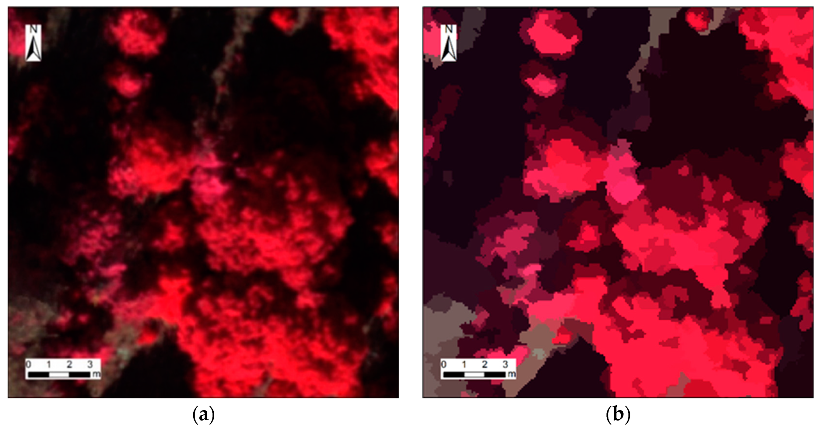
Figure 3.
Examples of tree characteristics by foliated evergreen oak in purple line and foliated pine in blue line observed in: (a) an RGB image; (b) an NIR image; and (c) spectral profiles of the two tree species in Codo study area.
Figure 3.
Examples of tree characteristics by foliated evergreen oak in purple line and foliated pine in blue line observed in: (a) an RGB image; (b) an NIR image; and (c) spectral profiles of the two tree species in Codo study area.

Figure 4.
Comparison of: (a) CIR image and (b) segmentation of the CIR-derived pixels that are similar in spectral properties as image objects.
Figure 4.
Comparison of: (a) CIR image and (b) segmentation of the CIR-derived pixels that are similar in spectral properties as image objects.

Figure 5.
Comparison of: (a) RGB image with a line of sight in red line and (b) corresponding point cloud profile of RGB-derived DSM.
Figure 5.
Comparison of: (a) RGB image with a line of sight in red line and (b) corresponding point cloud profile of RGB-derived DSM.

Figure 6.
The valley detection thresholding to separate shadow class toward the lowest NIR values in a multimodal distribution, with pixel intensity on the x-axis and frequency on the y-axis, in the four study areas: (a) Codo; (b) Hostal; (c) Bosquet; and (d) Olius.
Figure 6.
The valley detection thresholding to separate shadow class toward the lowest NIR values in a multimodal distribution, with pixel intensity on the x-axis and frequency on the y-axis, in the four study areas: (a) Codo; (b) Hostal; (c) Bosquet; and (d) Olius.

Figure 7.
The valley detection thresholding to separate foliated class towards the highest VI values in a multimodal distribution, with pixel intensity on the x-axis and frequency on the y-axis, for detecting defoliation in the Codo study area with: (a) NDVI; (b) GNDVI; (c) GRNDVI; and (d) NDVIRE.
Figure 7.
The valley detection thresholding to separate foliated class towards the highest VI values in a multimodal distribution, with pixel intensity on the x-axis and frequency on the y-axis, for detecting defoliation in the Codo study area with: (a) NDVI; (b) GNDVI; (c) GRNDVI; and (d) NDVIRE.

Figure 8.
The valley detection thresholding to discriminate pine toward lower VI values from evergreen oak, with pixel intensity on the x-axis and frequency on the y-axis, in the Codo study area with: (a) NDVI; (b) GNDVI; (c) GRNDVI; and (d) NDVIRE.
Figure 8.
The valley detection thresholding to discriminate pine toward lower VI values from evergreen oak, with pixel intensity on the x-axis and frequency on the y-axis, in the Codo study area with: (a) NDVI; (b) GNDVI; (c) GRNDVI; and (d) NDVIRE.

Figure 9.
Process of histogram thresholding analysis in Codo: (a) CIR image; (b) CIR image with NIR highlighting shadow pixels in gray; (c) CIR image with GNDVI highlighting foliated pixels in green and defoliated in meshed yellow; and (d) CIR image with GNDVI highlighting foliated pines in blue, foliated evergreen oaks in purple, and defoliated in meshed yellow. The process of Random Forest classification in Codo: (e) CIR-derived segmentation as image objects and (f) supervised Random Forest classifying shadow in gray, defoliated in yellow, pine in blue, and evergreen oak in purple.

Figure 10.
Sensitivity analysis testing the robustness of best performed VIs: (a) NDVI and (b) NDVIRE for defoliation detection in the four study areas. The optimal thresholds were highlighted in pink resulting in slightly lower values than the estimated average drawn in red line.
Figure 10.
Sensitivity analysis testing the robustness of best performed VIs: (a) NDVI and (b) NDVIRE for defoliation detection in the four study areas. The optimal thresholds were highlighted in pink resulting in slightly lower values than the estimated average drawn in red line.


Table 1.
RGB and NIR imagery features for orthomosaic generation in the Agisoft PhotoScan.
| Site | Codo | Hostal | Bosquet | Olius | ||||
|---|---|---|---|---|---|---|---|---|
| RGB | NIR | RGB | NIR | RGB | NIR | RGB | NIR | |
| Date (dd/mm/yy) | 26/11/2017 | 19/01/2018 | 23/01/2018 | 30/01/2018 | ||||
| Time (duration) | 12:43–12:50 | 12:05–12:14 | 12:16–12:22 | 11:55–12:03 | ||||
| Elevation (m) | 1300 | 820 | 620 | 720 | ||||
| Flight height (m) | 95 | 78 | 76 | 85 | ||||
| Area (ha) | 14.1 | 16.2 | 7.4 | 26.3 | ||||
| Number of images | 210 | 333 | 155 | 344 | ||||
| Data size (GB) | 0.93 | 0.49 | 1.65 | 0.78 | 0.39 | 0.36 | 1.05 | 0.80 |
| Processing time (h) | 4.8 | 3.3 | 7.6 | 5.0 | 3.9 | 2.4 | 5.7 | 3.8 |
| Software platform | Microsoft Windows 7 (64 bits) | |||||||
| Ground resolution (cm/pix) | 2.32 | 8.64 | 1.90 | 6.82 | 1.80 | 6.58 | 2.12 | 7.49 |
| RMS re-projection error (pix) | 2.45 | 0.66 | 2.51 | 0.70 | 2.34 | 0.64 | 2.19 | 0.62 |
Table 2.
Vegetation indices derived from UAS multispectral bands.
| Index | Acronym | Formula | |
|---|---|---|---|
| Normalized Difference Vegetation Index | NDVI | [42] | |
| Green Normalized Difference Vegetation Index | GNDVI | [41] | |
| Green–Red Normalized Difference Vegetation Index | GRNDVI | [43] | |
| Normalized Difference Vegetation Index Red Edge | NDVIRE | [44] |
Table 3.
Summary of threshold values determined by multimodal histogram distributions with various indices for classifying shadow, defoliated, and tree species.
Table 3.
Summary of threshold values determined by multimodal histogram distributions with various indices for classifying shadow, defoliated, and tree species.
| Classification | Index | Codo | Hostal | Bosquet | Olius | Total Average |
|---|---|---|---|---|---|---|
| Shadow | NIR | 17 | 23 | 27 | 28 | 24 |
| Defoliated | NDVI | 0.584 | 0.529 | 0.481 | 0.490 | 0.52 |
| GNDVI | 0.561 | - | - | 0.393 | - | |
| GRNDVI | 0.295 | 0.254 | 0.171 | 0.175 | 0.22 | |
| NDVIRE | 0.515 | 0.475 | 0.416 | 0.431 | 0.46 | |
| Species | NDVI | - | - | - | - | - |
| GNDVI | 0.681 | - | - | 0.631 | - | |
| GRNDVI | 0.539 | - | - | - | - | |
| NDVIRE | - | - | - | - | - |
Table 4.
Confusion matrix of NIR for shadow removal in the four study areas with the total of 400 randomly selected pixels, referenced to RGB images as ground observations.
Table 4.
Confusion matrix of NIR for shadow removal in the four study areas with the total of 400 randomly selected pixels, referenced to RGB images as ground observations.
| Class | Predicted | ||||
|---|---|---|---|---|---|
| Shadow | Sun | Total | Producer’s Accuracy | ||
| Observed | Shadow | 167 | 13 | 180 | 93% |
| Sun | 8 | 212 | 220 | 96% | |
| Total | 175 | 225 | 400 | ||
| User’s Accuracy | 95% | 94% | 95% | ||
Table 5.
Summary of overall accuracies from the confusion matrix of NIR in the four study areas for shadow removal, with each 100 randomly selected pixels referenced to ground observations.
Table 5.
Summary of overall accuracies from the confusion matrix of NIR in the four study areas for shadow removal, with each 100 randomly selected pixels referenced to ground observations.
| Index | Codo | Hostal | Bosquet | Olius | Total |
|---|---|---|---|---|---|
| NIR | 96% | 93% | 96% | 94% | 95% |
Table 6.
Summary of overall accuracies from the confusion matrix of four VIs in the four study areas for defoliation detection, with each 100 randomly selected pixels referenced to ground observations.
Table 6.
Summary of overall accuracies from the confusion matrix of four VIs in the four study areas for defoliation detection, with each 100 randomly selected pixels referenced to ground observations.
| Index | Codo | Hostal | Bosquet | Olius | Total |
|---|---|---|---|---|---|
| NDVI | 93% | 91% | 97% | 98% | 95% |
| GNDVI | 91% | - | - | 86% | - |
| GRNDVI | 93% | 84% | 95% | 97% | 92% |
| NDVIRE | 94% | 90% | 97% | 97% | 95% |
Table 7.
Summary of overall accuracies from the confusion matrix of GNDVI in the Codo and Olius study areas for species discrimination, with each 100 randomly selected pixels referenced to ground observations.
Table 7.
Summary of overall accuracies from the confusion matrix of GNDVI in the Codo and Olius study areas for species discrimination, with each 100 randomly selected pixels referenced to ground observations.
| Index | Codo | Hostal | Bosquet | Olius | Total |
|---|---|---|---|---|---|
| GNDVI | 96% | - | - | 93% | - |
Table 8.
Summary of overall accuracies from the confusion matrix of Random Forest classification in Codo study area for shadow, defoliated, and species, with 100 randomly selected pixels referenced to ground observations.
Table 8.
Summary of overall accuracies from the confusion matrix of Random Forest classification in Codo study area for shadow, defoliated, and species, with 100 randomly selected pixels referenced to ground observations.
| Class | Predicted | ||||||
|---|---|---|---|---|---|---|---|
| Shadow | Defoliated | Pine | Oak | Total | Producer’s Accuracy | ||
| Observed | Shadow | 22 | 1 | 3 | 0 | 26 | 85% |
| Defoliated | 0 | 31 | 0 | 0 | 31 | 100% | |
| Pine | 0 | 1 | 21 | 2 | 24 | 88% | |
| Oak | 0 | 0 | 0 | 19 | 19 | 100% | |
| Total | 22 | 33 | 24 | 21 | 100 | - | |
| User’s Accuracy | 100% | 94% | 88% | 90% | - | 93% | |
Table 9.
Summary of overall accuracies from the confusion matrix of Random Forest classification in Olius study area for shadow, defoliated, and species, with 100 randomly selected pixels referenced to ground observations.
Table 9.
Summary of overall accuracies from the confusion matrix of Random Forest classification in Olius study area for shadow, defoliated, and species, with 100 randomly selected pixels referenced to ground observations.
| Class | Predicted | ||||||
|---|---|---|---|---|---|---|---|
| Shadow | Defoliated | Pine | Oak | Total | Producer’s Accuracy | ||
| Observed | Shadow | 22 | 1 | 1 | 0 | 24 | 92% |
| Defoliated | 0 | 26 | 0 | 0 | 26 | 100% | |
| Pine | 0 | 2 | 26 | 0 | 28 | 93% | |
| Oak | 4 | 0 | 1 | 17 | 22 | 77% | |
| Total | 26 | 29 | 28 | 17 | 100 | - | |
| User’s Accuracy | 85% | 90% | 93% | 100% | - | 91% | |
© 2019 by the authors. Licensee MDPI, Basel, Switzerland. This article is an open access article distributed under the terms and conditions of the Creative Commons Attribution (CC BY) license (http://creativecommons.org/licenses/by/4.0/).
Share and Cite
MDPI and ACS Style
Otsu, K.; Pla, M.; Duane, A.; Cardil, A.; Brotons, L. Estimating the Threshold of Detection on Tree Crown Defoliation Using Vegetation Indices from UAS Multispectral Imagery. Drones 2019, 3, 80. https://doi.org/10.3390/drones3040080
AMA Style
Otsu K, Pla M, Duane A, Cardil A, Brotons L. Estimating the Threshold of Detection on Tree Crown Defoliation Using Vegetation Indices from UAS Multispectral Imagery. Drones. 2019; 3(4):80. https://doi.org/10.3390/drones3040080
Chicago/Turabian StyleOtsu, Kaori, Magda Pla, Andrea Duane, Adrián Cardil, and Lluís Brotons. 2019. "Estimating the Threshold of Detection on Tree Crown Defoliation Using Vegetation Indices from UAS Multispectral Imagery" Drones 3, no. 4: 80. https://doi.org/10.3390/drones3040080