Accuracy Assessment of 3D Photogrammetric Models from an Unmanned Aerial Vehicle

Abstract

The unmanned aerial vehicle (UAV) photogrammetric survey of an archaeological site has proved itself to be particularly efficient. In order to obtain highly accurate and reliable results, it is necessary to design carefully the flight plan and the geo-referencing, while also evaluating the indicators of the accuracy rate. Using as a test case a UAV photogrammetric survey conducted on the archaeological site of the Roman Amphitheatre of Avella (Italy), in this paper, we propose a pipeline to assess the accuracy of the results according to some quality indicators. The flight configuration and the georeferencing chosen is then be checked via the residuals on the ground control points (GCPs), evenly distributed on the edges and over the entire area. With the aim of appraising the accuracy of the final model, we will suggest a method for the outlier detection, taking into account the statistical distribution (both global and of portion of the study object) of the reprojection errors. A filter to reduce the noise within the model will then be implemented through the detection of the angle formed by homologous rays, in order to reach a compromise between the number of the usable points and the reduction of the noise linked to the definition of the 3D model.

1. Introduction

Over the last decade, the use of photogrammetry for the acquisition of digital 3D models has undergone a significant increase in its applications. In fact, thanks to the evolution of algorithms from computer vision and new computation techniques, factors that were once known to be weak points of the technique including photogrammetric image processing, now take less time and are mostly automated [1].

Over time, there has been a gradual evolution from the use of dense point clouds acquired with laser scanner technology, common in many 3D surveying applications, to an increasing use of photogrammetry, thanks to the introduction of automatic Structure from Motion (SfM) technology [2].

The factors that have favoured the unmanned aerial vehicle (UAV) acquisition technique, compared to the terrestrial laser scanner (TLS) technique, are mainly: a lower cost of the instrument, a higher speed of data acquisition and, above all, a better texture of the 3D model, useful also for a correct analysis and archaeological characterization [3,4]. The disadvantages of UAVs include the limitation of the payload, the reduced autonomy and the greater dependence on climatic conditions (e.g., wind) [5,6].

From 2000 onwards, drones have become increasingly used for aerial photogrammetry applications and the first studies on the quality of the results were published in those years [7]; more recently, the technological development of UAVs, which are becoming easier to drive and more reliable, has indirectly favoured the increase of photogrammetric applications, especially for medium and large scale.

An advantage of UAV-borne sensors is the ability to acquire data at close range from multiple angles of view. In literature the classification of UAV images is mainly in two groups: nadir images, where the axis of the camera is vertical, and oblique images, taken with a tilted camera (generally at 45°). Generally, a nadir view, commonly used in photogrammetry, produced greater occlusion and some details may be lost; the combined use of nadir and oblique images has the advantage of improving the definition of shapes, the continuity of surfaces and a better description of sub-vertical walls [8].

Currently, the photogrammetric technique has gained even more vitality, probably exceeding range-based sensors in the number of surveying applications [9].

The photogrammetric applications in the civil field of UAVs are many and widely documented in the literature; among these: high-resolution reconstruction of the land surface for geomorphological analysis and for monitoring purposes [10,11]; studies on agriculture and forests through the analysis of multispectral images [12,13]; and the management of disasters immediately after a catastrophic event [14]. UAVs are also widely used in the infrastructure sector, for example to inspect towers and bridges [15], for air transport infrastructure [16], and for railways and roads [17].

However, it is especially in the field of cultural heritage (CH) that UAV photogrammetry is applicable for a variety of different purposes [18]. The technique is indeed very versatile because of the speed of acquisition and the transportability of the vehicle, allowing the use of these instruments for different applications [19]; in the literature it is possible to find applications for the structural monitoring of historical buildings [20], for the generation of 3D models to be used for the computation of volumes and for the subsequent generation of metric drawings for representation purposes, for the estimation of excavations [21] and also for the mapping of the degradation of the facades of historical buildings [22,23].

In the literature, there are also numerous examples of UAV systems used for photogrammetric purposes in the archaeological field for the three-dimensional survey of complex structures such as the Roman Amphitheatre in Pompeii [24,25], and outside the Italian context, the Ancient Nikopolis Theatre in Greece [26] or the Carnuntum Amphitheatre in Austria [27].

This clearly shows that the UAV can be a key factor in making quick and accurate decisions, overcoming the limitations and problems of data acquisition and processing, which is very costly and time-consuming [28,29]. In this regard, Stoker et al. [30] provided a detailed overview of the variety of remote sensing applications based on the use of UAV, deepening the current status of the Federal Aviation Administration (FAA) Regulations.

In most cultural heritage documentation applications, cameras installed on UAVs are often commercial, non-calibrated (reflex or mirrorless) cameras. It is always good practice to acquire a much higher number of images than strictly necessary, to avoid data holes in the model, and to improve the success of the matching and the subsequent alignment of the images. In terms of processing time, a higher number of images does not significantly increase the computation time.

In most photogrammetric applications, self-calibration is a standard procedure, providing better metric results [31]. The scale of representation of the graphic drawings of the object surveyed by photogrammetry techniques often does not include an accuracy analysis. From the definition of graphical error, it can only be deduced that the maximum scale of representation is inversely proportional to the errors related to the processing of the model [32].

Low accuracy in model building may nullify the high resolution of the data and, as a result, the graphical scale of output products, such as plans and sections, must be smaller. It is therefore necessary to validate the data obtained by analysing some photogrammetric parameters that influence the process of model reconstruction. It is not trivial to underline that, depending on the final purpose of the photogrammetric survey, the accuracy required in data acquisition and processing is different; if you want to produce for example a 3D model for augmented reality (AR), or make simple web visualizations, meaning non-scientific applications, the estimation of the accuracy of the model can be left out.

It is especially in the field of AR that you can find various tools for online viewing and editing of the photogrammetric model. These tools can help some professionals with dissemination and documentation in the field of CH, for purposes such as the creation of virtual museums or remote knowledge of archaeological sites that are not so well known or are difficult to reach [33,34,35,36]. The use of drones in this field is not limited to 3D modelling only, but is a powerful tool to virtually visit the area of interest.

On the contrary, in the overall field of CH, where the purpose is the conservation and/or monitoring of archaeological heritage or architectural restoration, the evaluation of metric accuracy is necessary to avoid producing documents that are ‘incorrect’ from a metric point of view. In the analysis of accuracy, it is not possible to generalize the rules for choosing the optimal parameters of acquisition regardless of the object of interest.

From the literature, it is clear that the accuracy of the model is dependent on certain photogrammetric parameters. Among those that most affect the accuracy of the output are:

• the angle formed between the homologous rays in the different shots; generally, the greater this angle (within a certain interval), the greater the achievable accuracy, as Krauss studies show a direct proportionality between the base/height ratio and accuracy [37];
• the measurement of ground control points (GCPs); for the same number, the measurement accuracy of GCPs is directly proportional to the accuracy of the photogrammetric model [10].

The methodology used to estimate the calibration parameters of the camera, which is generally performed in the laboratory, but can also be performed directly during the post-processing phase by applying the self-calibration procedures (although these procedures are usually less accurate) is also of great relevance for the achievable accuracy.

Evaluating the accuracy of a georeferenced 3D model can be done in several ways. A basic method is to analyse the residues of the bundle adjustment (BA) by computing the root mean squared error (RMSE) of the residues on the GCPs or by using the coordinates measured on the ground independently of the points with which to compare the coordinates measured on the photogrammetric model (check point) [38].

Camera positions derived from the SfM algorithm do not have the scale and orientation provided by GCP coordinates; as a result, the 3D point cloud is generated in relative coordinates, referred to the image coordinate system. Georeferencing of this model is generally done using a small number of GCPs located at clearly visible positions both on the ground and in the photographs; it is necessary to carry out a detailed study of the positions of the GCPs in order to maximize the accuracy obtained from the photogrammetric projects.

Harwin and Lucieer [39] note that the number and distribution of GCPs have an effect on the accuracy of the model. All photogrammetric users agree that a configuration with many points evenly distributed over the surveyed area is optimal; for optimal results in planimetry, it is essential to place the GCPs at the edge of the study area. However, this point configuration does not optimize altimetry results [40]. Some researchers compared different software products for generating 3D point clouds and noted that the differences in results also depend on the software used [41]; flight altitudes also influence the quality of the model [42].

This work is the continuation of a previous research, published in [43], which had as its main purpose to verify which method of image acquisition and which modality of Global Positioning Satellite System (GNSS) survey of the GCPs allowed to produce the best 3D model, from which to derive traditional graphic designs, at the scales of representation commonly used.

The present work focuses on the quality analysis of the best model obtained with the best technique previously identified.

The sparse point cloud, made only by tie points (TPs), is the starting point for the realization of the complete 3D model; however, the presence of low quality TPs is evident, and their removal is appropriate because their presence affects the results of the next steps, which consist of the recomputation of the orientation parameters, and the creation of the final dense cloud.

Most of the photogrammetric software provides the possibility to filter the TPs based on the estimate of the reprojection error associated with each of them. In our work, we wanted to deepen the contribution of the reprojection error but also took into account the geometry of acquisition by studying the correlation between the mean value of the angles formed by the homologous rays that intersect on the TPs and the noise on the creation of the model. Some points, potential outliers, can be removed by analysing the frequency distribution of the reprojection errors on the basis of the confidence interval, obtained experimentally on our data.

In this note we propose an algorithm for the calculation of roughness on the sparse point cloud that can be studied in relation to the associated angular interval.

2. Case Study and Data Acquisition

2.1. The Roman Amphitheatre of Avella (Italy)

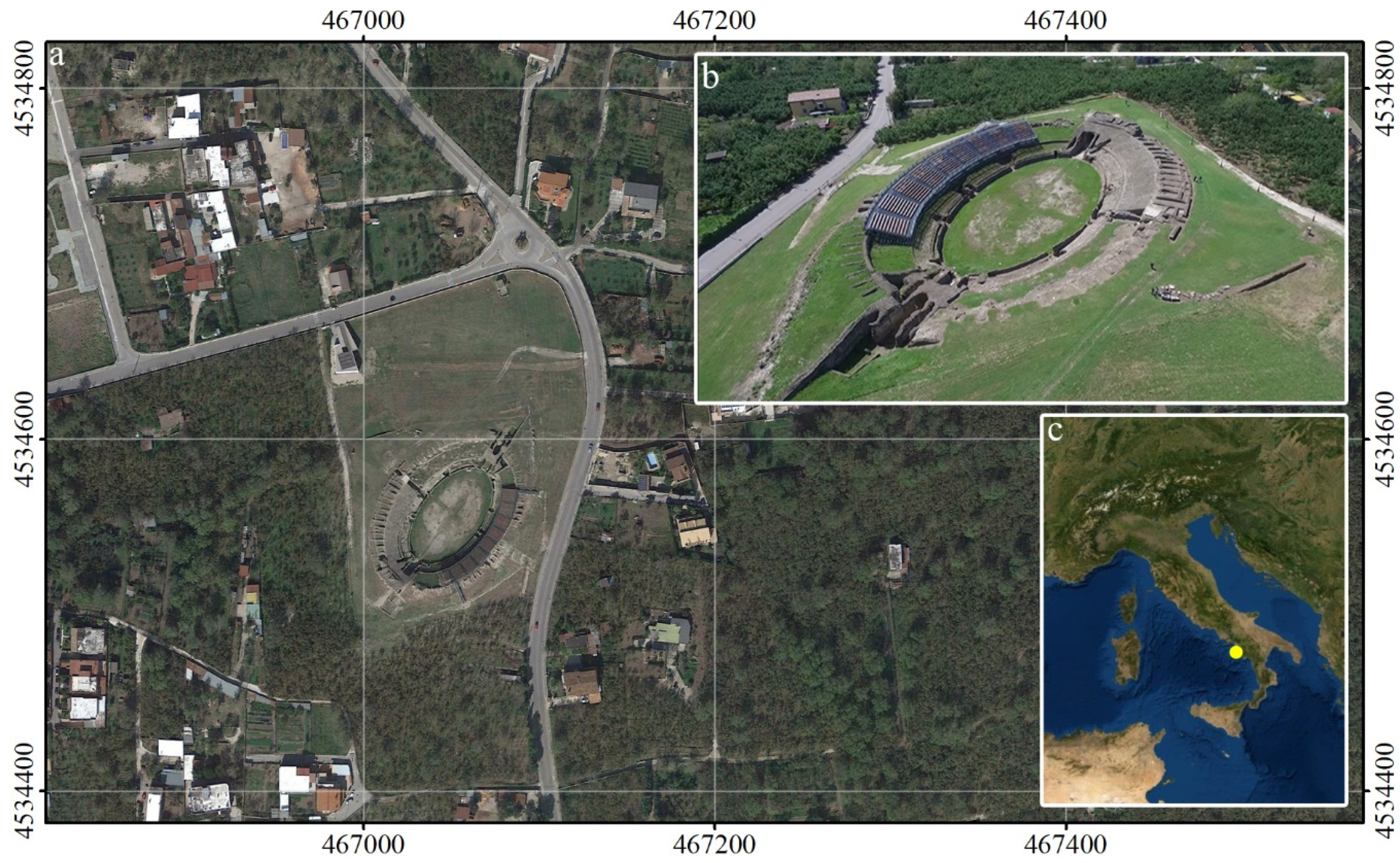
Considering the archaeological traces, the Amphitheatre of Avella (Figure 1) can be dated between the end of the 8th and the beginning of the 7th century BC. The Amphitheatre, is similar in composition to the complex located in Pompeii, and is one of the oldest in Campania, and in Italy [44]. Unlike other more recent sites, like the Colosseum in Rome or the Flavio Amphitheatre in Pozzuoli, there are no underground passages and there are only two monumental entrances, consisting of vaulted hallways in the ‘opus caementicium’ placed on opposite sides of the main axis. The structure consists of two external semi-circular structures joined by orthogonal walls and of an internal oval-shaped arena, which covers an area of 63.6 $\times$ 34.3 m.

The ‘cavea’ is developed on three orders: the ‘ima cavea’, the ‘media cavea’, and the ‘summa cavea’. The other few remains are located on the south and east sides, while the ‘media cavea’, is divided into three parts (moeniana, praecintiones and baltei). These are still in a good state of preservation.

The idea of performing a 3D digitization of the Amphitheatre was born in early 2016 when there was a survey, study and analysis of the archaeological site was carried out as part of the Project ‘The Amphitheatre of Avella, from its origins to the digital: architecture, landscape, virtual representation, innovations for knowledge and fruition’.

A detailed and precise digital acquisition and 3D modelling of the Amphitheatre was decided upon, aimed at using different 3D recording technologies and modelling techniques. Due to the high metric quality of the required documents, it was necessary to pay attention to the metric error of the photogrammetric model, with particular importance on an accurate topographic measurements made during the campaign phase.

The project purpose is a first digitization of the Amphitheatre; a cartographic output (consisting of plans and sections) at a scale 1:100 and 1:50 will be produced starting from the final 3D model, to document in the current conservation status. In agreement with the ‘Soprintendenza Archeologica, Belle Arti e Paesaggio per le province di Salerno e Avellino’, an average spatial resolution of 10 mm for the 3D model was then chosen, since it was considered sufficient to their aims.

Obviously, lighter and simplified 3D models can be obtained from the highest resolution once subsampling methods were applied.

2.2. UAV Photogrammetric Flight

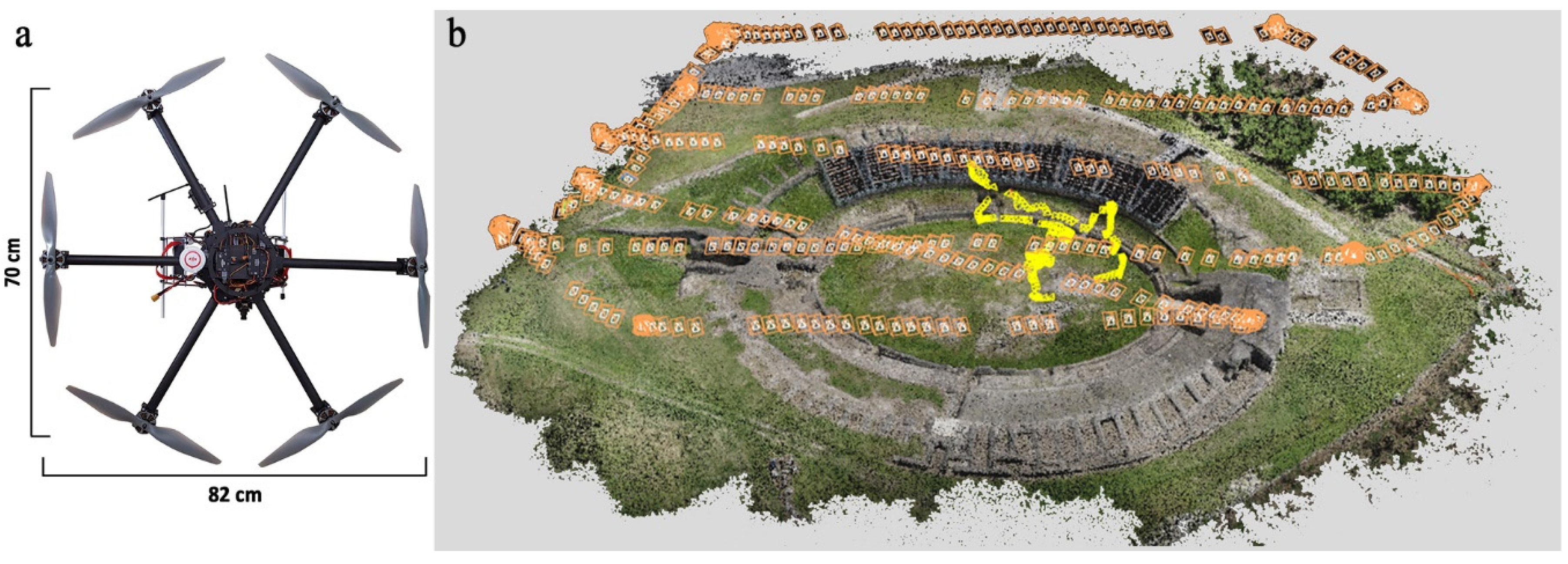
The UAV system used for this application is an assembled hexacopter (Figure 2a) with a net weight of the sensor of about 2.3 kg and maximum payload of 1 kg. The installed camera is a mirrorless Sony Nex 7 with 24-megapixel APS-C sensor (6000 $\times$ 4000 pixels, 23.5 $\times$ 15.6 mm and a Pixel Size of 3.96 μm) and a fixed Sony E-Mount lens (16 mm focal length, Field of View-FOV 83°).

The complete equipment uses several control boards and a complex set of sensors. In particular, the elements that characterize it are:

• a frame in carbon and fiberglass with six arms;
  six brushless motors 740 kV with and propellers 14 $\times$ 5 cm;
  six electronic speed controller circuits (ESCs) FullPower 40 A, that adjust the speed of rotation of motors;
• flight control (FC) DJI Wookong;
• remote control Graupner MX16 2.4 GHz (RC) that allows the gimbal control and the rotation of the camera along of the three axes;
• remote control Futaba 2.4 GHz S-FHSS that allows the driving of the vehicle, activates the different flight modes in remotely mode, sets and/or locks the flight height measured by the altimeter;
• three-axis Gimbal with brushless motors of the type iPower Motor GMB4008-150t, a servo-assisted support characterized by greater fluidity in the movements.

For the acquisition of the photogrammetric shots, a double capture mode was then selected. The first one using an automatic flight plan for the acquisition of nadir photogrammetric images and the second one using manual mode with the camera’s optical axis tilted at about 45°, to survey the vertical walls and any shadow cones present in the ‘cavea’.

The flight lines were designed using a DJI Ground-Station software package. For all surveys the UAV was set to a target altitude of 24 m above the take off point (32 m from arena plan) and horizontal ground speed of 3.0 m/s. The height is computed in the DJI Ground-Station software using elevation data derived from Google Earth. Parallel flight lines were programmed to have an image front-overlap of 80% and side-overlap of 60%, setting the proper camera parameters (dimensions of the sensor, focal length and flight height). Larger overlaps correspond to smaller base-lines, i.e., smaller intersection angles which result in lower accuracy [37].

The frequency of the intervallometer has been set to acquire images every 2 s along the parallel flight lines, resulting in the acquisition of an image about every 6 m along the flight lines. The camera was set to aperture priority mode and a diaphragm aperture of f/8 for nadir images and f/5.6 for oblique ones have been used, where the f is the focal length.

The UAV had a flight-time of ~8 min whilst carrying its payload (using two lithium polymer battery, 11 Ah, 22.2 V, 6 cel. A generous overhead, ~4 min, was left in order to safely land the UAV). In Italy, unaided visual line of sight (VLOS) have to be maintained whilst operating UAV [45].

The image acquisition was planned bearing in mind the project requirements—a ground sampling distance (GSD) of about 1 cm - and, at the same time, with the aim of guaranteeing a high level of automation in the following step of the data elaboration.

The total amount of acquired images is 626, of which, 435 were by automatic flight plan and camera in nadir, while the remaining 191 were taken with a manual flight and optical camera axis tilted at 45°. The nadir flight was developed from the northwest to southeast, which provides a ground coverage of about 47.0 $\times$ 31.2 m. The manual flight was carried out with a tilted camera and an average height of flight of 21 m, which provides an inconstant ground coverage, ranging between 16.0 $\times$ 11.0 m and 23.5 $\times$ 15.6 m, respectively.

The acquired images were processed in a single project, containing both nadir (425) and oblique images (191). Figure 2b shows the position of the photogrammetric shots, in orange the images acquired in nadir with automatic flight plan, in yellow the oblique images acquired in manual mode.

2.3. GCPs Acquisition

To georeference the photogrammetric shots three GCP networks surveyed with GNSS (Global Navigation Satellite System) techniques were used, one in fast-static and two in network Real Time Kinematic (nRTK). A GNSS receiver GEOMAX Zenith 25 Series in nRTK mode and a Trimble 5700 GPS receiver in fast-static mode were used.

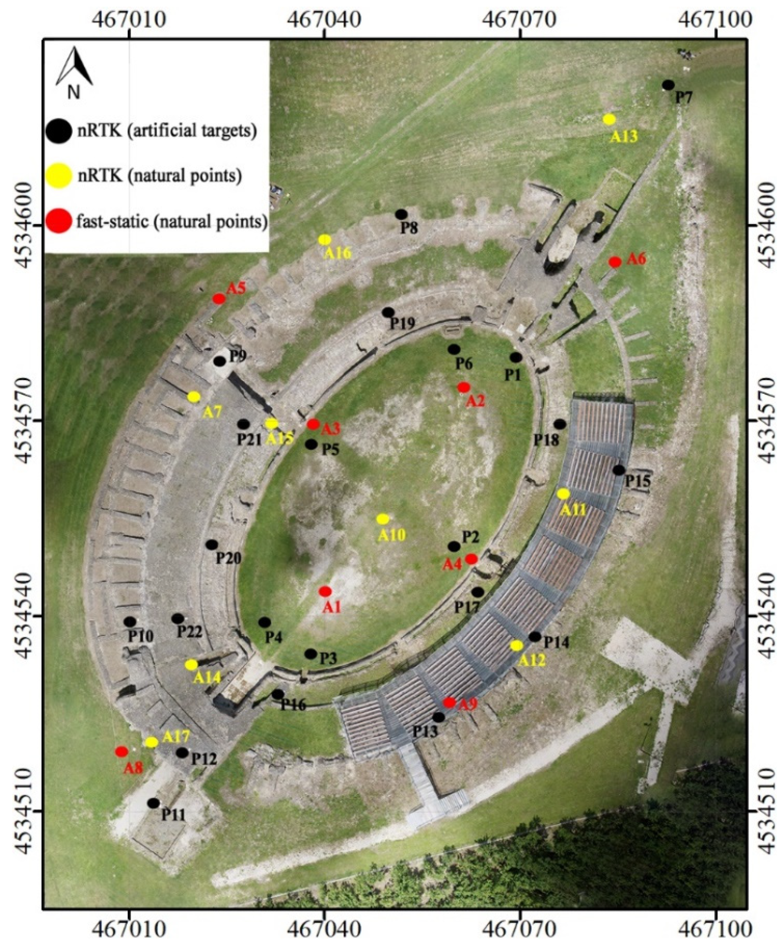
In UAV photogrammetry, the best solution is to distribute the GCPs uniformly, both at the edges and within the area [40]. The spatial distribution of the GCPs in the three configurations is shown in Figure 3. The fast-static network is composed of eight vertices, which are natural points clearly identified, the well distributed spatially and altimetrically (A1-A8, in red). The two nRTK networks are made up of seventeen natural points (A1-A17, in yellow) and twenty-two artificial coded targets [46] (42 $\times$ 29.7 cm, format A3, P1-P22, in black) respectively. Eight points (from A1 to A8) are in common for the first two networks.

The GNSS survey refers to the Italian geodetic and cartographic System UTM/ETRF00 [47] through a connection to two permanent stations (AVEL and ROBS) included in the national Geodetic Network located within a radius of 10 km from the test area. A new point (master) has been materialized near the Amphitheatre and connected to the permanent stations with static baselines.

3. Methods

The level of accuracy that one tries to obtain is proportional to both the scale of representation, and the graphic error. Therefore, it is essential to verify the entity.

According to Padua et al. [48], to obtain more details and to generate a more accurate 3D model, it is more appropriate to also acquire oblique images. To decide which is the best set of data in terms of accuracy, the data of two different photogrammetric configurations have been analysed:

• only nadir images;
• both nadir and oblique images.

To georeference the images, in both cases the GCPs, consisting of natural points on the ground and photogrammetric targets, were measured with GNSS receivers in fast-static and nRTK modalities.

Once the best data set has been selected, a more detailed accuracy analysis of the final 3D model was performed, analysing a number of quality features of the sparse 3D point cloud. The following quality features analysed in greater detail:

• the residual on the image coordinates, also called ‘reprojection errors’, computed in the georeferencing phase, starting with the result of the adjustment of the GNSS measurements; they represent the accuracy of the computation of each tie point belonging to the sparse cloud;
• the angle between the homologous rays of all tie points for each pair of images and the average of the angle values;
• the number of images (image count) used to estimate the position of each tie point.

After the analysis of both the residuals on GCPs and the error projection, only the configuration that optimizes these two parameters will be further analysed with the evaluation of angles and image count. The objective is to evaluate the influence of these parameters within the photogrammetric process by applying the appropriate filters to remove noise.

To evaluate the effectiveness of the noise reduction the surface roughness was estimated by applying a least squares plane fitting interpolation to the points of the cloud within a sphere of fixed radius. The corresponding RMSE value derived from the interpolation is then associated with each point of the cloud. The averages frequency distributions, is a better interpolate the RMSE values, have been correlated with the filtering parameters used.

Finally, a correlation analysis between the computed quality features will be carried out, to analyse the relationships that exist between them.

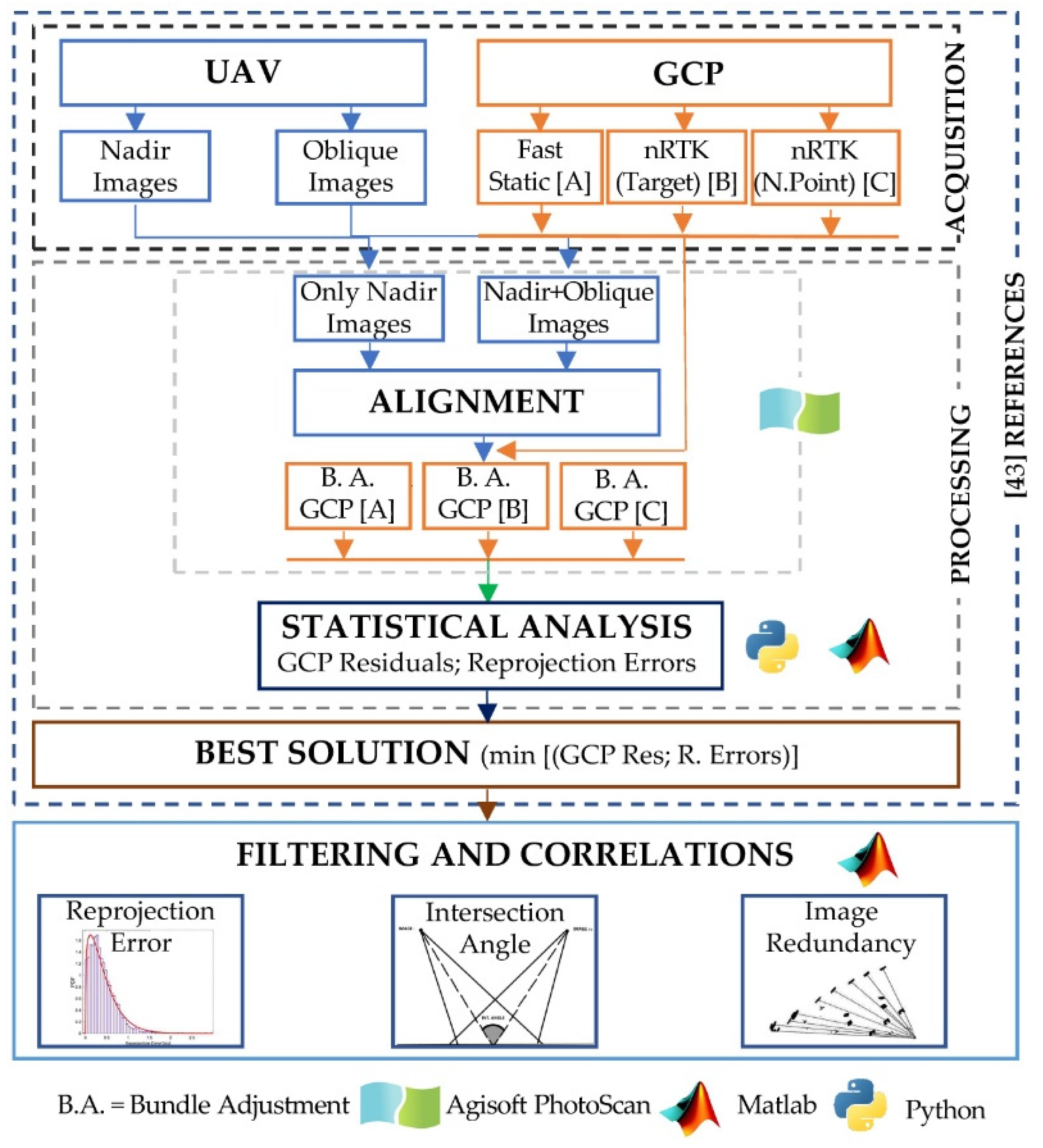
Figure 4 shows a flow chart of the data processing, including those analysed in the reference work [43].

3.1. Data Elaboration

In order to process the photogrammetric data, PhotoScan software package by Agisoft (ver. 1.4.2 build 4164, 2017) has been used [49].

The interior orientation parameters were estimated in PhotoScan using a self-calibrating bundle adjustment by including the GCPs. This strategy was chosen as each SfM tool provided different solutions to estimate the camera calibration. Therefore, it is important that the calibration software used to estimate the parameters employs the same mathematical model as the one used for bundle adjustment. These estimated parameters were then used to orient the images. Additionally, the estimated parameters were kept constant during the entire SfM processing.

The following parameters were set to build the sparse cloud consisting of tie-points: in the ‘Align Photos’ phase, accuracy = high (original photos), key point limit = 4000, tie point limit = no.

To carry out the tests, a Dell precision tower 3620 workstation, 32 Gb Ram, 500 Gb SSD storage, Intel Xeon E3 1200 V5 processor and a Radeon Pro WX5100 GPU were used.

A first estimate of the quality of the georeferencing is given by the residuals on the GCPs and the associated RMSE [10]:

$$\begin{array}{l}RMS{E}_E=\sqrt{\frac{1}{n}\cdot {\displaystyle \sum _{i=1}^n{\left({\overline{E}}_{Ci}-E_{Ri}\right)}^2}}\\ RMS{E}_N=\sqrt{\frac{1}{n}\cdot {\displaystyle \sum _{i=1}^n{\left({\overline{N}}_{Ci}-N_{Ri}\right)}^2}}\\ RMS{E}_h=\sqrt{\frac{1}{n}\cdot {\displaystyle \sum _{i=1}^n{\left({\overline{h}}_{Ci}-h_{Ri}\right)}^2}}\\ RMSE=\sqrt{RMS{E}_E^2+RMS{E}_N^2+RMS{E}_h^2}\end{array}$$

(1)

where the subscript C indicates the coordinates estimated from the bundle adjustment, R indicates the reference values, E and N are respectively the East, North cartographic coordinates, h is the ellipsoidal height, and n indicates the number of GCPs.

The next step was the building of the dense cloud, we used the following parameters: quality = high (1/4 of original photos), depth filtering = disable.

Once the photogrammetric image processing is complete, the textured 3D model used to extract the nadir orthophoto was created. The orthophoto will then be vectorised to draw the plan of the Amphitheatre of Avella.

3.2. Reprojection Error

The reprojection error is a geometric error corresponding to the image distance between a projected point and a measured one [50]. It is used to quantify how closely an estimate of a 3D point recreates the point’s true projection.

For the computation of the 3D coordinates of a tie point, the parameters of inner and external orientation of the camera and the image coordinates of the point are used. Once its coordinates are computed, the 3D point is reprojected on all the images where it appears. The distance between the image-point and the reprojected point on a single image is the reprojection error. This error is also referred to as RMS image residual [50]. Mathematically, the reprojection error is obtained as follows:

$$w\left(\begin{array}{c}u\\ v\\ 1\end{array}\right)=\left(\begin{array}{ccc}{f}_u& 0& u_c\\ 0& f_v& v_c\\ 0& 0& 1\end{array}\right)\left(R_c^T-R_c^T{t}_c\right)\left(\begin{array}{c}P\\ 1\end{array}\right)=K{P}_c\left(\begin{array}{c}P\\ 1\end{array}\right)$$

(2)

where: f_u and f_v are the focal lengths in u and v directions and [u_c,v_c] is the principal point offset, t_c is the position of the camera centre in an object space, R_c is the rotation from the camera back to the object frame and K is the matrix of interior parameters. P is the vector containing the coordinates p_i of the projective space. The product KP_c represents the projective matrix.

$${\epsilon }_i=\left(\begin{array}{c}{u}_i\\ v_i\end{array}\right)-{\left[\left(\begin{array}{ccc}0& 0& 1\end{array}\right)K{P}_c\left(\begin{array}{c}{p}_i\\ 1\end{array}\right)\right]}^{-1}\left(\begin{array}{ccc}1& 0& 0\\ 0& 1& 0\end{array}\right)K{P}_c\left(\begin{array}{c}{p}_i\\ 1\end{array}\right)$$

(3)

Each tie point extracted is associated with a reprojection error value ε_i, which is the module of the sum of the reprojection errors computed for the number of cameras that see the i-th tie point.

In addition, using a Matlab tool (i.e., Statistics toolbox), the frequency distribution of the reprojection errors that best fits the data has been studied. The distribution was used to remove external values at a chosen experimental threshold, which are considered outliers. The tie points corresponding to threshold values that identify them as TPs have been removed using an algorithm implemented in Python environment.

3.3. Angle Between Homologous Points

It is known that one of the parameters that most influences the accuracy of a photogrammetric project is the base/height ratio [37].

In this paper, the analysis on base/height ratio was carried out by estimating the angle between two projecting lines (called the ‘intersection angle’). The photogrammetric software we used does not give the value of this angle in output, so we implemented an algorithm in the Python environment.

For the extraction and computation of the parameters of interest, two libraries have been used: NumPy [51], a library for adding support for large, multi-dimensional arrays and matrices, along with a large collection of high-level mathematical functions to operate on these arrays; Pandas [52], an open source, Berkeley Software Distribution (BSD) licensed library providing high-performance, easy-to-use data structures.

The input parameters used to compute the intersection angles are:

• projection centre (O);
• tie point (k).

Given the k-th tie point seen from two images i and j, the direction vectors u_i and v_j are given by the relations:

$$\begin{array}{l}{u}_i=\left[E_{Oi}-E_k;N_{Oi}-N_k;h_{Oi}-h_k\right]\\ v_j=\left[E_{Oj}-E_k;N_{Oj}-N_k;h_{Oj}-h_k\right]\end{array}$$

(4)

where the subscript O_i indicates the projection centre of the i-th frame and O_j of the j-th frame, E, N, h are the cartographic coordinates.

The relation gives the intersection angle α:

$$\cos \alpha =\frac{u\cdot v}{\left|u\right|\cdot \left|v\right|}$$

(5)

The estimate of the intersection angle has been made using all the pairs of frames that see the i-th tie point, computing for each pair the intersection angle and finally computing the average intersection angle between the n frames that show the point, eliminating the extreme values. Finally, the process associates the average angular value obtained with each tie point extracted. The whole process is implemented in Python.

4. Result and Discussion

4.1. Results of the GNSS Survey

The five hours spent to connect the master station to the permanent stations has ensured high precision in the position of the points, 4 mm in planimetry and 10 mm in altimetry.

From the master station to the GCPs, the distance was less than 50 m and the baselines were measured with sessions lasting longer than 30 minutes. The computation of the baselines produced RMS in the order of 5 mm in planimetry and 12 mm in height. The GCP positions obtained with static baselines represent the reference values to evaluate the accuracy of the measurements in nRTK mode. The absolute values of the differences in coordinates are on average 15 mm in planimetry and 26 mm in altimetry, the associated RMS is 9 mm and 12 mm respectively. Note that, the uncertainty associated with nRTK measurements was on average 8 mm in planimetry and 15 mm in elevation. This result confirms the reliability of the nRTK network in real time, and authorizes the use of the nRTK modality for positioning the remaining GCPs.

4.2. Building of the Sparse Point Cloud

Oblique images are useful to reduce the shadow areas in which data could not be acquired, as on vertical elements (i.e., walls). In our case study, the values of residuals on the GCPs are more dispersed when using both nadir and oblique images while they are less dispersed but higher if you use only the nadir images. Using photogrammetric artificial targets, the interquartile range is smaller, and the lowest residuals were obtained using the nadir image-only set. When using both nadir and oblique images, the test shows that the most accurate result is obtained using GCP surveys in fast-static, which is the most accurate survey modality.

For the nadir image-only set, the GNSS survey mode used has less influence; in fact, nRTK measurements, both on natural points and on photogrammetric targets, have an interquartile range and similar average residuals.

For the following phases of data extraction and analysis, the dataset used is complete, consisting of nadir and oblique images.

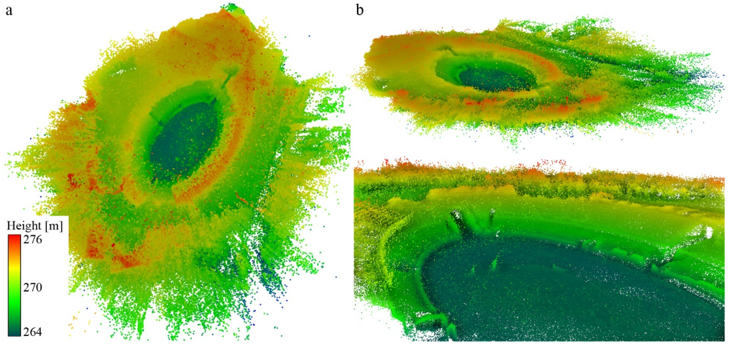
Figure 5 shows some views of the sparse cloud obtained with that data set. The point cloud has an average density of 400 points/m². It is possible to notice some errors (noise) on the arena and on the ‘cavea’ (lighter scattered points). It is clear that the sparse point clouds need to be filtered out before the final computation of the orientation parameters can be made. The creation of the dense cloud must be done with the parameters estimated using the sufficiently accurate tie points.

4.3. Reprojection Error

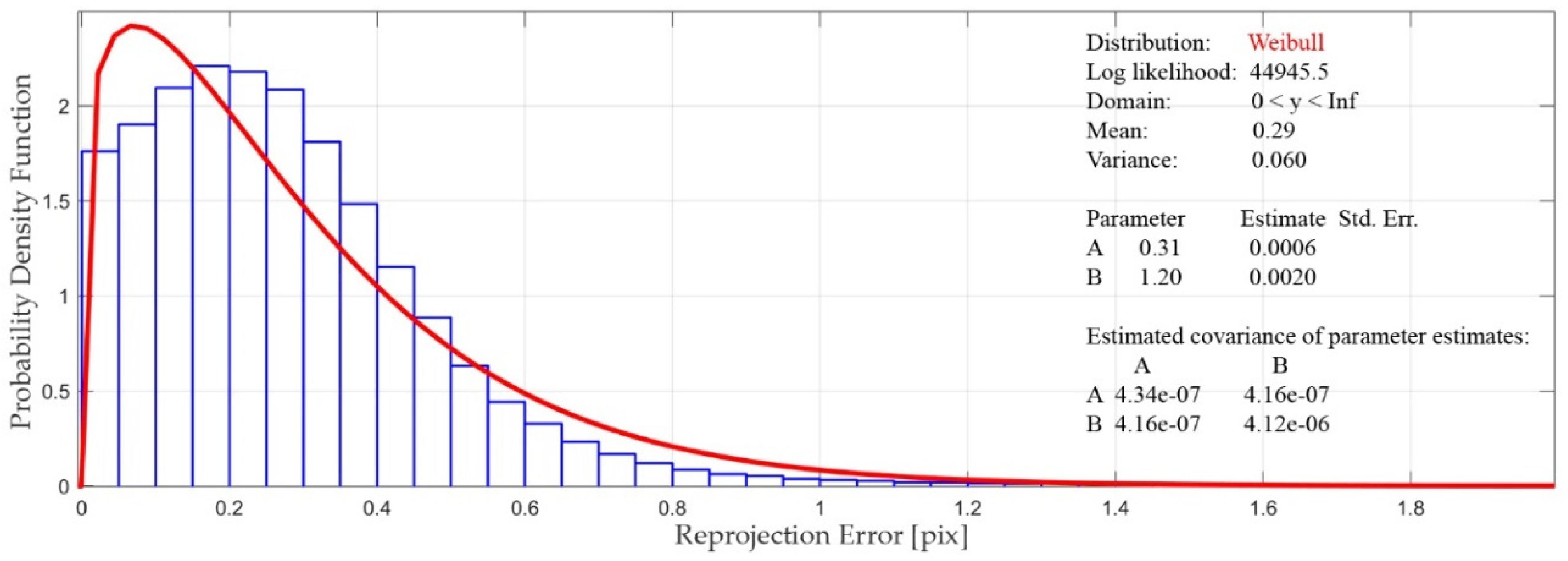
The frequency distribution that best fits the data (the reprojection errors) is the Weibull distribution (Figure 6). Also for these errors the chosen configuration (data set consisting of nadir and oblique images, georeferenced with GCPs surveyed in fast-static) is the one that gave the best results (lowest errors) [43].

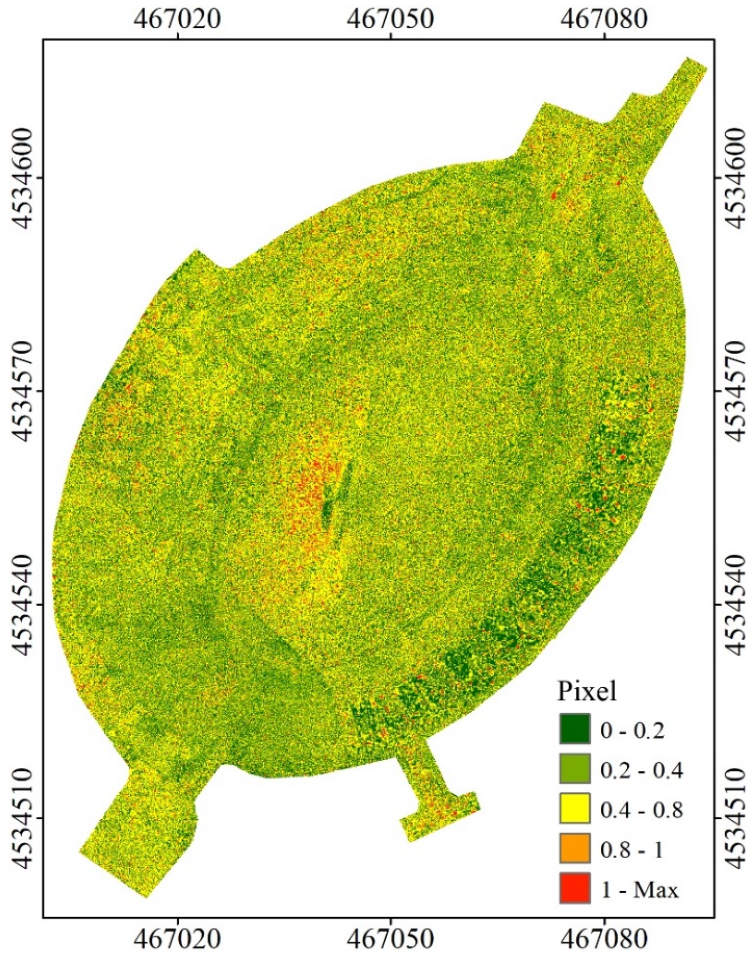
Figure 7 shows the classified map of the reprojection errors on the amphitheatre. The error pattern is very homogeneous; no areas with particular problems were identified, except for the south-western area of the arena. In the south-eastern area, at the metal steps, the distribution is more heterogeneous; this is mainly due to the presence of highly reflective material that produces more noise. For a more detailed analysis, it is necessary to concentrate on limited and significant portions of the structure.

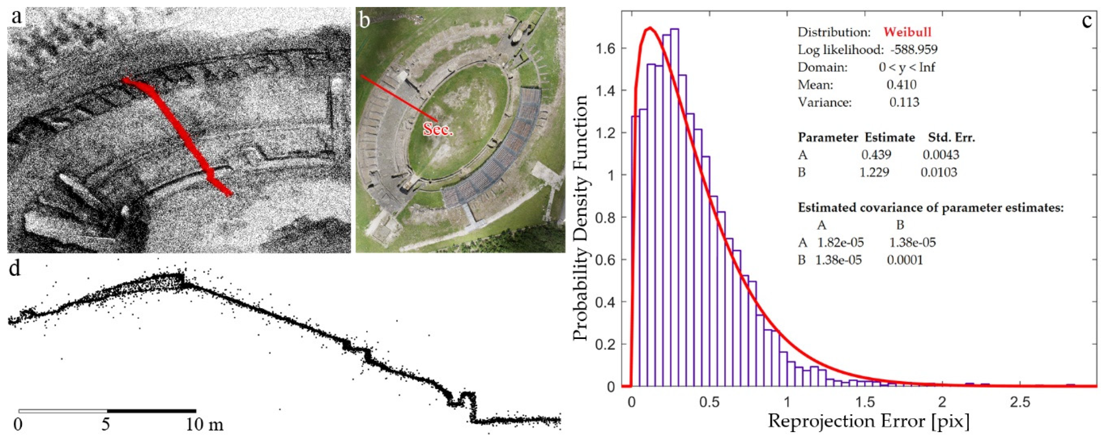
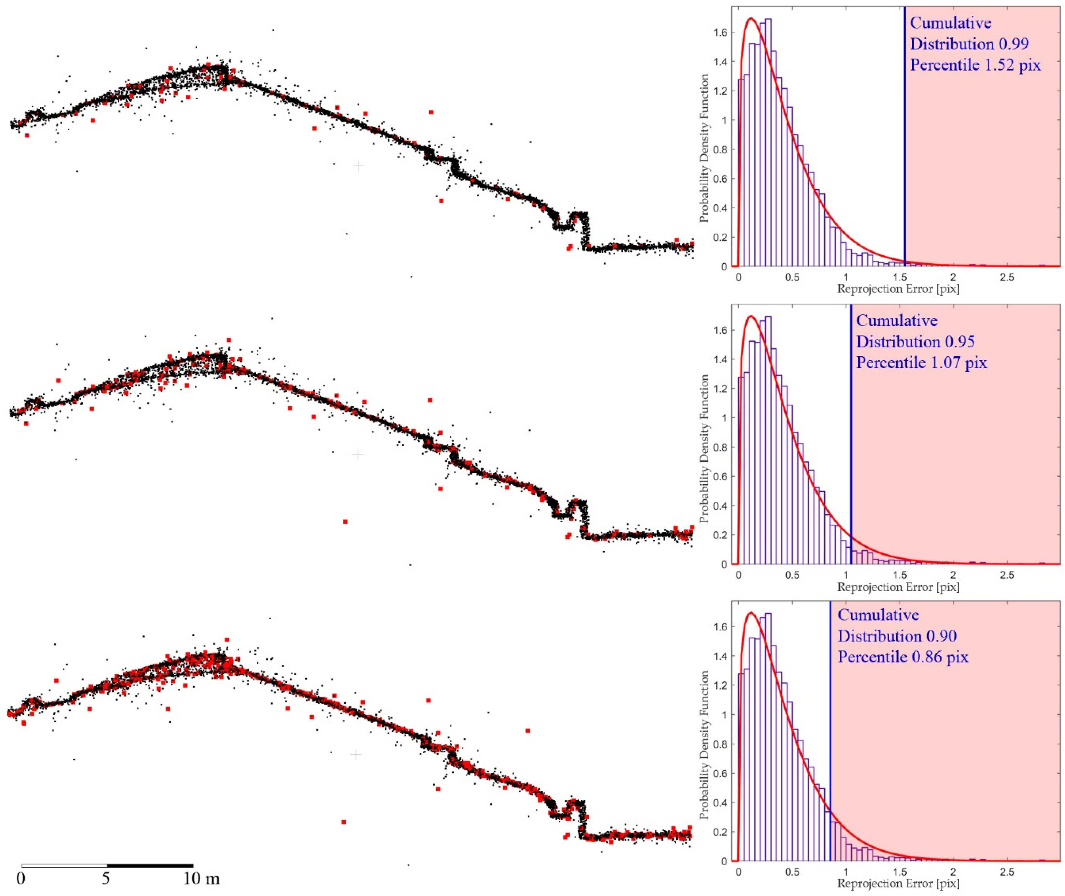
For the purpose of the analysis, a standard section was identified, 2 m wide (Figure 8a,b,d), very noisy, and containing part of the ‘cavea’, the arena and the vertical walls. The Weibull distribution interpolated the data, shape and scale parameters were estimated, with the uncertainties of the associated estimates (Figure 8c).

The study of the distribution was used to determine the threshold values, in order to remove the points with associated reprojection error values above the estimated threshold values. All points with error values higher than the ‘lower cumulative distribution’ were removed; in better detail, those higher than the 99th, 95th, and 90th percentile.

Observing Figure 9 it is possible to notice how filtering of the point cloud was done by analysing the reprojection error allows the removal of some points mostly scattered (in red in Figure 9) to be considered not to be representative of the trend of the structure, but does not lead to great advantages in reducing noise. However, most of the isolated points have not been filtered out.

4.4. Analysis of Angle Values between Homologous Rays

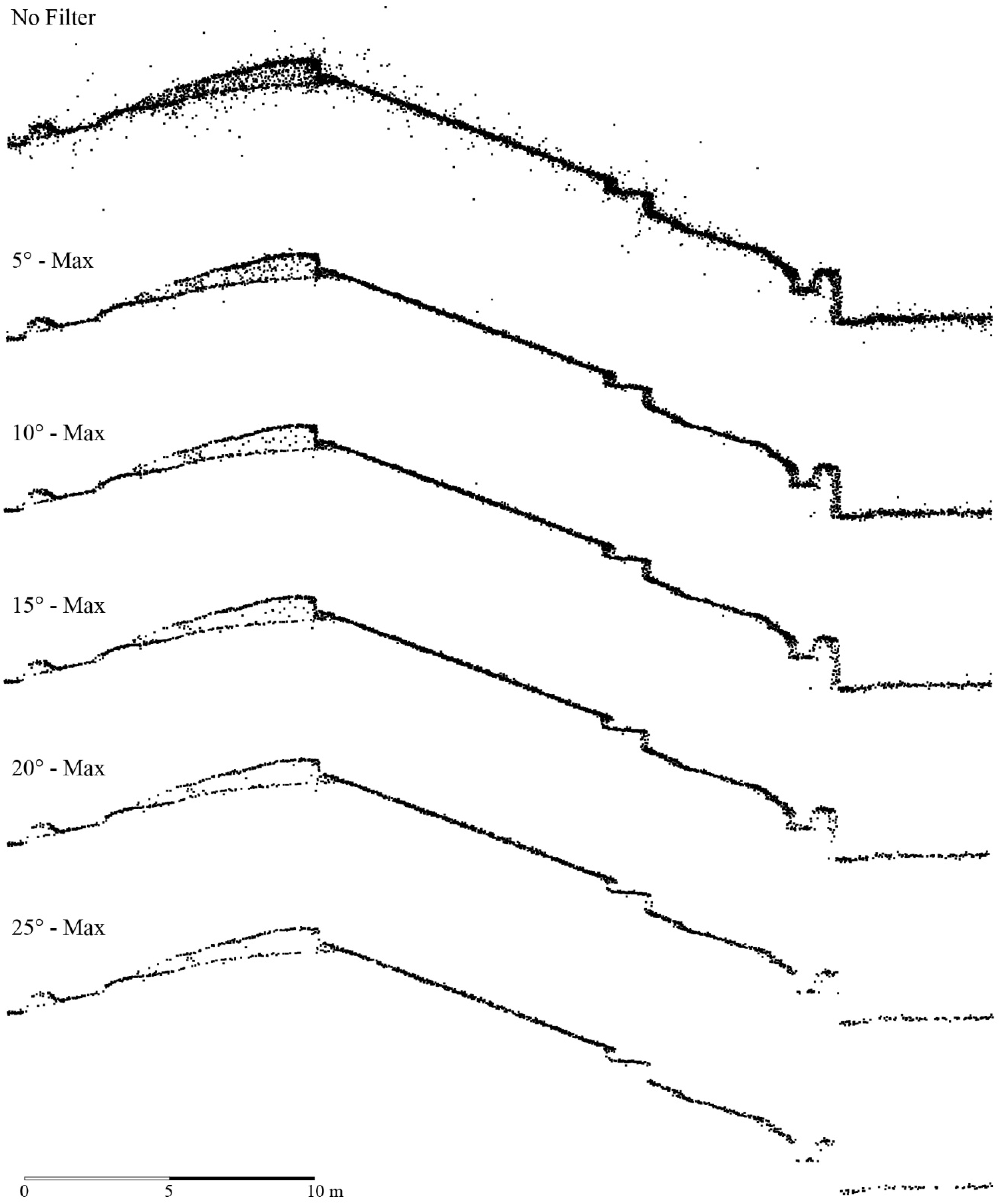
A better result for the reduction of ‘noise’, as computed by the method indicated above, are obtained by filtering the point cloud according to the average angle, computed for each tie point, and thus analysing the acquisition geometry. Figure 10 shows a cross-section filtered in steps of 5°.

Angles lower than 5° produce very noisy results since they derive from a very small base/height ratio. Therefore, excluding the step by step small angles, much more relevant and less noisy surfaces were obtained. Beyond 20°, the points belonging to the vertical face are removed, so no analysis with greater angles has been made.

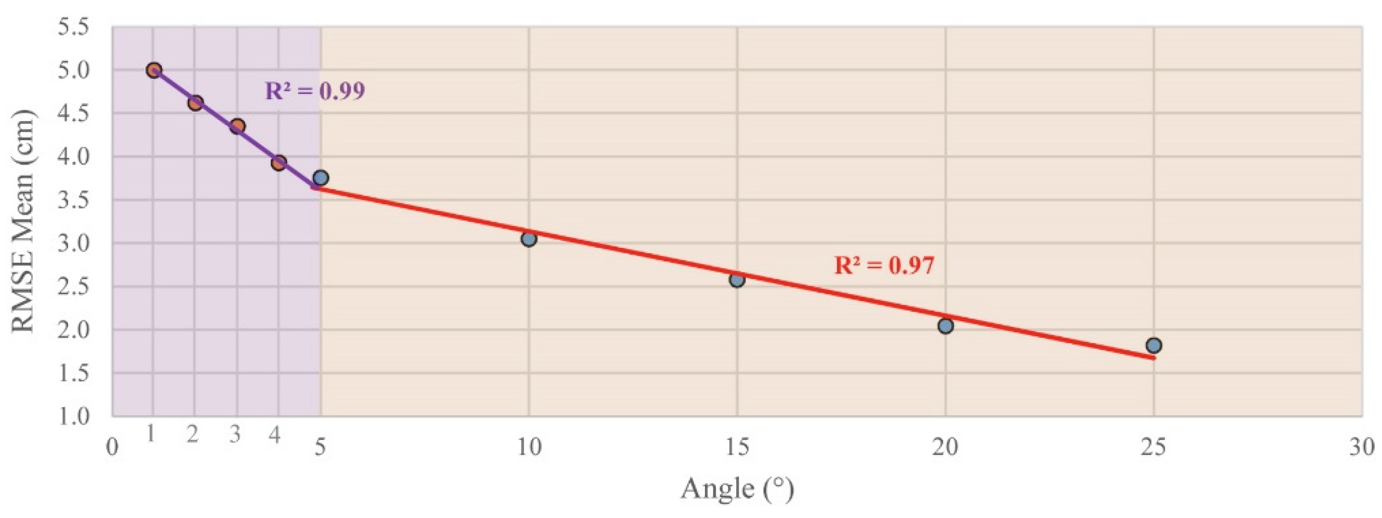
Figure 11 shows the trends of the average RMSE values obtained with the parameters used for the angle filter. The mean values of the distribution were calculated by interpolating a Burr type XII distribution, since it was the one that best fit the values of RMSE. The radius of the research sphere was set at 25 cm and therefore only the points deviating from the interpolated surface of this quantity are considered. In the case of the filter with reprojection error there are no benefits from the removal of noise; as the percentile used to estimate the threshold decreases and therefore the removal of extreme values, the average value of RMSE remains constant, around 5.2 cm. On the contrary, as the angle increases, the average value of RMSE decreases linearly. In Figure 11 it is possible to identify two sections; the first (from 1° to 4°) is strictly linear and has a greater slope than the second section (from 5° to 25°), which is also linear.

4.5. Correlation Analysis

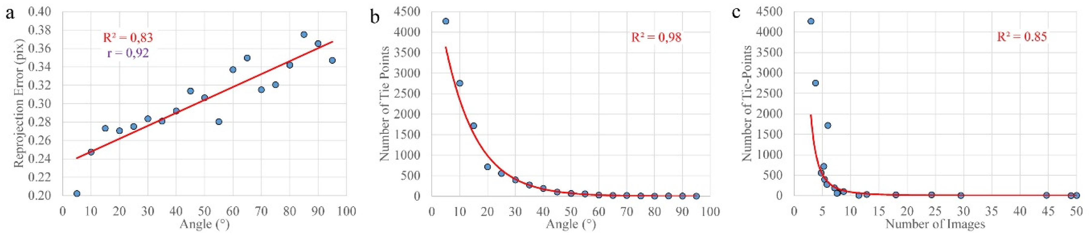
For the optimal configuration, the reprojection error values and the average angles have been related. The correlation is high and positive (Pearson Correlation greater than 0.9, Figure 12a). The graphs in Figure 12b,c have an exponential trend that shows the relationships between the number of tie points with the angle and the number of images used to generate that tie point. It should be noted that small angles are more frequent (Figure 12b), a symptom of a greater overlap of images. Also, tie points that are computed using very distant images and therefore with very high angles are rare. The number of images used to determine most of the tie points are small, indicating a higher frequency of small angles (Figure 12c).

The software used, PhotoScan, allows us to compute the position of all points that are visible on at least two images. The tie points visible only on two images will be located with a low value of accuracy. Counting the number of images used to compute the position of the tie points allows us to evaluate the quality of the 3D positioning of a point, which is also a function of an adequate value of angle between homologous rays.

The results allow us to say that, at least with reference to the dataset used, we are faced with two opposing needs: A high number of close images (very small angle values) allows the correlation of a very high number of tie points and therefore a detailed reconstruction of the object surveyed, so it is advisable to use a high number of images even very close. However, we can see that close images induce a strong noise and therefore a lower accuracy of interpolation, so it would be better to remove the images that are too close (i.e., small angles). The trend of the RMSE in function of the value of the minimum angle between images allowed as to remove close images (Figure 11) that can suggest the threshold value to choose, which for this dataset is 5°.

5. Conclusions

The UAV survey of the Avella Amphitheatre confirms the importance of good georeferencing to obtain sufficiently accurate results; the quality of this georeferencing can be verified using a sufficient number of uniformly distributed check points.

However, a careful analysis of the point cloud is also necessary to obtain high quality and reliable products. The quality of the point cloud has been verified on the basis of the computation of the reprojection error associated with each TP and the graphical visualization of the values of this error has highlighted the weak areas of the survey. The study of the frequency distribution of the values usually allows the identification of a statistical distribution (in this case a Weibull distribution) and the relative confidence interval (associated with a pre-selected confidence level), in order to consider the points falling out of the interval as outliers and to remove them from the TPs cloud. It has been helpful to take into account not only the global behaviour, but also some profiles corresponding to certain cross sections of the model that have been analysed in more detail.

The geometry of the acquisition of the frames has as known a huge impact on the precision of a photogrammetric survey, but, in the case of a UAV survey, the high number of shots functional to a good outcome of the correlation makes it difficult to identify the single images that have contributed to the determination of the position of each TP. The implementation of ad hoc algorithms has allowed us to extract the value of the angle formed by the homologous rays on each pair of images that ‘sees’ each TP; from the analysis of these values it has been possible to quantitatively evaluate that the close-up frames have led to the correlation of a large number of TPs, but also to the generation of a higher noise.

By analysing some profiles in detail, it was possible to fix an angle threshold value that determines the TPs to be removed to filter the noise, while maintaining a correct modelling of the object. The elimination of TPs strongly influences the computation of the orientation parameters. The update of the alignment computation and transformation parameters is based only on the remaining tie points. The next step will be to automatically filter the sparse cloud within the proprietary software. Once the noise has been reduced, a more accurate dense cloud will be produced. The product will be more suitable for automatic vectorization and mapping.

The proposed method is believed to be applicable in all cases involving similar structures, and we propose to apply the method to several test cases, partly already being studied.

References

- Falkingham, P.L. Acquisition of high resolution three-dimensional models using free, open-source, photogrammetric software. Palaeontol. Electron. 2011, 15, 1–15. [Google Scholar] [CrossRef]
- Baltsavias, E.P. A comparison between photogrammetry and laser scanning. Isprs J. Photogramm. Remote Sens. 1999, 54, 83–94. [Google Scholar] [CrossRef]
- Barba, S.; Barbarella, M.; Di Benedetto, A.; Fiani, M.; Limongiello, M. Comparison of UAVs performance for a Roman Amphitheatre survey: The case of Avella (Italy). In Proceedings of the 2nd International Conference of Geomatics and Restoration (Volume XLII-2/W11), Milan, Italy, 8–10 May 2019; pp. 179–186. [Google Scholar]
- Rinaudo, F.; Chiabrando, F.; Lingua, A.; Spanò, A. Archaeological site monitoring: UAV photogrammetry can be an answer. Int. Arch. Photogramm. Remote Sens. Spat. Inf. Sci. 2012, XXXIX-B5, 583–588. [Google Scholar] [CrossRef]
- Pflimlin, J.M.; Soueres, P.; Hamel, T. Hovering flight stabilization in wind gusts for ducted fan UAV. In Proceedings of the 2004 43rd IEEE Conference on Decision and Control (CDC) (IEEE Cat. No.04CH37601), Nassau, Bahamas, 14–17 December 2004; pp. 3491–3496. [Google Scholar]
- Zongjian, L. UAV for mapping—low altitude photogrammetric survey. Int. Arch. Photogramm. Remote Sens. Beijingchina 2008, 37, 1183–1186. [Google Scholar]
- Eisenbeiß, H. UAV Photogrammetry. Ph.D. Thesis, Institut für Geodesie und Photogrammetrie, ETH-Zürich, Zürich, Switzerland, 2009. [Google Scholar]
- Rossi, P.; Mancini, F.; Dubbini, M.; Mazzone, F.; Capra, A. Combining nadir and oblique UAV imagery to reconstruct quarry topography: Methodology and feasibility analysis. Eur. J. Remote Sens. 2017, 50, 211–221. [Google Scholar] [CrossRef]
- Remondino, F.; Barazzetti, L.; Nex, F.; Scaioni, M.; Sarazzi, D. UAV photogrammetry for mapping and 3D modeling – current status and future perspectives. Isprs - Int. Arch. Photogramm. Remote Sens. Spat. Inf. Sci. 2012, XXXVIII-1-C22, 25–31. [Google Scholar] [CrossRef]
- Agüera-Vega, F.; Carvajal-Ramírez, F.; Martínez-Carricondo, P. Assessment of photogrammetric mapping accuracy based on variation ground control points number using unmanned aerial vehicle. Measurement 2017, 98, 221–227. [Google Scholar] [CrossRef]
- Rossi, G.; Tanteri, L.; Tofani, V.; Vannocci, P.; Moretti, S.; Casagli, N. Multitemporal UAV surveys for landslide mapping and characterization. Landslides 2018, 15, 1045–1052. [Google Scholar] [CrossRef] [Green Version]
- Feng, Q.; Liu, J.; Gong, J. UAV Remote Sensing for Urban Vegetation Mapping Using Random Forest and Texture Analysis. Remote Sens. 2015, 7, 1074–1094. [Google Scholar] [CrossRef] [Green Version]
- Honkavaara, E.; Saari, H.; Kaivosoja, J.; Pölönen, I.; Hakala, T.; Litkey, P.; Mäkynen, J.; Pesonen, L. Processing and Assessment of Spectrometric, Stereoscopic Imagery Collected Using a Lightweight UAV Spectral Camera for Precision Agriculture. Remote Sens. 2013, 5, 5006–5039. [Google Scholar] [CrossRef] [Green Version]
- Quaritsch, M.; Kruggl, K.; Wischounig-Strucl, D.; Bhattacharya, S.; Shah, M.; Rinner, B. Networked UAVs as aerial sensor network for disaster management applications. e & i Elektrotechnik Und Inf. 2010, 127, 56–63. [Google Scholar]
- Morgenthal, G.; Hallermann, N.; Kersten, J.; Taraben, J.; Debus, P.; Helmrich, M.; Rodehorst, V. Framework for automated UAS-based structural condition assessment of bridges. Autom. Constr. 2019, 97, 77–95. [Google Scholar] [CrossRef]
- Mualla, Y.; Najjar, A.; Galland, S.; Nicolle, C.; Tchappi, I.H.; Yasar, A.-U.-H.; Främling, K. Between the Megalopolis and the Deep Blue Sky: Challenges of Transport with UAVs in Future Smart Cities. In Proceedings of the 18th International Conference on Autonomous Agents and MultiAgent Systems, Montreal QC, Canada, 13–17 May 2019; pp. 1649–1653. [Google Scholar]
- Máthé, K.; Buşoniu, L. Vision and Control for UAVs: A Survey of General Methods and of Inexpensive Platforms for Infrastructure Inspection. Sensors 2015, 15, 14887–14916. [Google Scholar] [CrossRef] [PubMed] [Green Version]
- Themistocleous, K.; Ioannides, M.; Agapiou, A.; Hadjimitsis, D.G. The methodology of documenting cultural heritage sites using photogrammetry, UAV, and 3D printing techniques: The case study of Asinou Church in Cyprus. In Proceedings of the Third International Conference on Remote Sensing and Geoinformation of the Environment, 2015, Paphos, Cyprus, 22 June 2015. [Google Scholar] [CrossRef]
- Fernández-Hernandez, J.; González-Aguilera, D.; Rodríguez-Gonzálvez, P.; Mancera-Taboada, J. Image-Based Modelling from Unmanned Aerial Vehicle (UAV) Photogrammetry: An Effective, Low-Cost Tool for Archaeological Applications. Archaeometry 2015, 57, 128–145. [Google Scholar] [CrossRef]
- Arias, P.; Herráez, J.; Lorenzo, H.; Ordóñez, C. Control of structural problems in cultural heritage monuments using close-range photogrammetry and computer methods. Comput. Struct. 2005, 83, 1754–1766. [Google Scholar] [CrossRef]
- Bendea, H.; Chiabrando, F.; Tonolo, F.G.; Marenchino, D. Mapping of archaeological areas using a low-cost UAV. The Augusta Bagiennorum test site. In Proceedings of XXI International CIPA Symposium, Athens, Greece, 1–6 October 2007. [Google Scholar]
- Brunetaud, X.; Luca, L.D.; Janvier-Badosa, S.; Beck, K.; Al-Mukhtar, M. Application of digital techniques in monument preservation. Eur. J. Environ. Civil. Eng. 2012, 16, 543–556. [Google Scholar] [CrossRef]
- Themistocleous, K. Model reconstruction for 3D vizualization of cultural heritage sites using open data from social media: The case study of Soli, Cyprus. J. Archaeol. Sci. Rep. 2017, 14, 774–781. [Google Scholar] [CrossRef]
- Fiorillo, F.; De Feo, E.; Musmeci, D. The architecture, geometry and representation of the Amphitheatre of Pompeii. In The reasons of Drawing; Gangemi Editore: Rome, Italy, 2016; pp. 1143–1146. [Google Scholar]
- Nocerino, E.; Menna, F.; Remondino, F.; Saleri, R. Accuracy and block deformation analysis in automatic UAV and terrestrial photogrammetry-Lesson learnt. Isprs Ann. Photogramm. Remote Sens. Spat. Inf. Sci. 2013, 2, 203–208. [Google Scholar] [CrossRef]
- Bilis, T.; Kouimtzoglou, T.; Magnisali, M.; Tokmakidis, P. The use of 3D scanning and photogrammetry techniques in the case study of the Roman Theatre of Nikopolis. Surveying, virtual reconstruction and restoration study. Int. Arch. Photogramm. Remote Sens. Spat. Inf. Sci. 2017, XLII-2/W3, 97–103. [Google Scholar] [CrossRef]
- Verhoeven, G.; Docter, R. The amphitheatre of Carnuntum: Towards a complete 3D model using airborne Structure from Motion and dense image matching. In Proceedings of the 10th International Conference on Archaeological Prospection, Vienna, Austria, 29 May–2 June 2013; Austrian Academy of Sciences: Vienna, Austria; pp. 438–440. [Google Scholar]
- Segales, A.; Gregor, R.; Rodas, J.; Gregor, D.; Toledo, S. Implementation of a low cost UAV for photogrammetry measurement applications. In Proceedings of the 2016 International Conference on Unmanned Aircraft Systems (ICUAS), Arlington, VA, USA, 7–10 June 2016; pp. 926–932. [Google Scholar]
- Templin, T.; Popielarczyk, D.; Kosecki, R. Application of Low-Cost Fixed-Wing UAV for Inland Lakes Shoreline Investigation. Pure Appl. Geophys. 2018, 175, 3263–3283. [Google Scholar] [CrossRef]
- Stöcker, C.; Bennett, R.; Nex, F.; Gerke, M.; Zevenbergen, J. Review of the Current State of UAV Regulations. Remote Sens. 2017, 9, 459. [Google Scholar] [CrossRef]
- Remondino, F.; Fraser, C. Digital camera calibration methods: Considerations and comparisons. Int. Arch. Photogramm. Remote Sens. Spat. Inf. Sci. 2006, 36, 266–272. [Google Scholar]
- Cardone, V. Modelli Grafici Dell’architettura e del Territorio; Maggioli Editore: Santarcangelo di Romagna, Italy, 2015. [Google Scholar]
- Kim, S.J.; Jeong, Y.; Park, S.; Ryu, K.; Oh, G. A Survey of Drone use for Entertainment and AVR (Augmented and Virtual Reality). In Augmented Reality and Virtual Reality: Empowering Human, Place and Business; Springer: Berlin, Germany, 2018; pp. 339–352. [Google Scholar]
- Marques, L.; Tenedório, J.A.; Burns, M.; Romão, T.; Birra, F.; Marques, J.; Pires, A. Cultural Heritage 3D Modelling and visualisation within an Augmented Reality Environment, based on Geographic Information Technologies and mobile platforms. Archit. City Environ. 2017, 11, 117–136. [Google Scholar]
- Olalde, K.; García, B.; Seco, A. The Importance of Geometry Combined with New Techniques for Augmented Reality. Procedia Comput. Sci. 2013, 25, 136–143. [Google Scholar] [CrossRef] [Green Version]
- Thon, S.; Serena-Allier, D.; Salvetat, C.; Lacotte, F. Flying a drone in a museum: An augmented-reality cultural serious game in Provence. In Proceedings of the 2013 Digital Heritage International Congress (DigitalHeritage), 28 October–1 November 2013; pp. 669–676. [Google Scholar]
- Kraus, K. Photogrammetry: Geometry from Images and Laser Scans; Walter de Gruyter: Berlin, Germay, 20 November 2007. [Google Scholar]
- Sanz-Ablanedo, E.; Chandler, J.H.; Rodríguez-Pérez, J.R.; Ordóñez, C. Accuracy of Unmanned Aerial Vehicle (UAV) and SfM Photogrammetry Survey as a Function of the Number and Location of Ground Control Points Used. Remote Sens. 2018, 10, 1606. [Google Scholar] [CrossRef]
- Harwin, S.; Lucieer, A. Assessing the Accuracy of Georeferenced Point Clouds Produced via Multi-View Stereopsis from Unmanned Aerial Vehicle (UAV) Imagery. Remote Sens. 2012, 4, 1573–1599. [Google Scholar] [CrossRef] [Green Version]
- Martínez-Carricondo, P.; Agüera-Vega, F.; Carvajal-Ramírez, F.; Mesas-Carrascosa, F.-J.; García-Ferrer, A.; Pérez-Porras, F.-J. Assessment of UAV-photogrammetric mapping accuracy based on variation of ground control points. Int. J. Appl. Earth Obs. Geoinf. 2018, 72, 1–10. [Google Scholar] [CrossRef]
- Neitzel, F.; Klonowski, J. Mobile 3D mapping with a low-cost UAV system. Int. Arch. Photogramm. Remote Sens. Spat. Inf. Sci. 2012, XXXVIII-1/C22, 39–44. [Google Scholar] [CrossRef]
- Anders, N.; Masselink, R.; Keesstra, S.; Suomalainen, J. High-res digital surface modeling using fixed-wing UAV-based photogrammetry. In Proceedings of the Geomorphometry 2013, Nanjing, China, 16–20 October 2013; pp. 16–20. [Google Scholar]
- Barba, S.; Barbarella, M.; Di Benedetto, A.; Fiani, M.; Limongiello, M. Quality assessment of UAV photogrammetric archaeological survey. Int. Arch. Photogramm. Remote Sens. Spat. Inf. Sci. 2019, XLII-2/W9, 93–100. [Google Scholar] [CrossRef]
- Limongiello, M.; Santoriello, A.; Schirru, G.; Bonaudo, R.; Barba, S. The Amphitheatre of Avella: From its origin to digital. In Proceedings of the IMEKO International Conference on Metrology for Archaeology and Cultural Heritage, Torino, Italy, 19–21 October 2016. [Google Scholar]
- ENAC. LG 2016/003-NAV Aeromobili a Pilotaggio Remoto con Caratteristiche di Inoffensività. 2016. Available online: https://www.enac.gov.it/la-normativa/normativa-enac/linee-guida/lg-2016003-nav (accessed on 15 October 2019).
- Ahn, S.J.; Rauh, W. Circular Coded Target and Its Application to Optical 3D-Measurement Techniques. In Proceedings of the Mustererkennung 1998, Berlin, Heidelberg, 29 September–1 October 1998; pp. 245–252. [Google Scholar]
- Barbarella, M. Digital technology and geodetic infrastructures in Italian cartography. Città E Stor. 2014, 9, 91–110. [Google Scholar]
- Pádua, L.; Adão, T.; Hruška, J.; Marques, P.; Sousa, A.; Morais, R.; Lourenço, J.M.; Sousa, J.J.; Peres, E. UAS-based photogrammetry of cultural heritage sites: A case study addressing Chapel of Espírito Santo and photogrammetric software comparison. In Proceedings of the International Conference on Geoinformatics and Data Analysis, Prague, Czech Republic, 15–17 March 2019; pp. 72–76. [Google Scholar]
- Agisoft, L. Agisoft PhotoScan user manual. Prof. Ed. Version 2016, 1, 37. [Google Scholar]
- James, M.R.; Robson, S.; d’Oleire-Oltmanns, S.; Niethammer, U. Optimising UAV topographic surveys processed with structure-from-motion: Ground control quality, quantity and bundle adjustment. Geomorphology 2017, 280, 51–66. [Google Scholar] [CrossRef] [Green Version]
- Oliphant, T. NumPy. Available online: https://numpy.org/ (accessed on 1 February 2019).
- McKinney, W. Pandas. Available online: https://pandas.pydata.org/ (accessed on 1 February 2019).
Figure 1.
Test area: (a) location map; (b) the Amphitheatre of Avella (Italy); (c) the test area in the South of Italy.
Figure 2.
(a) UAV System; (b) Camera positions: in orange the nadir images (by flight plan), in yellow the oblique images (by manual piloting).
Figure 3.
Spatial distribution of the ground control points (GCPs). Network real time kinematic (nRTK).
Figure 4.
Flow-chart.
Figure 5.
The sparse point cloud and the chromatic scale is a function of the elevation values. (a) Top view. (b) Perspective views.
Figure 6.
Weibull distribution for the reprojection errors.
Figure 7.
Classified map of the reprojection errors.
Figure 8.
(a) Cross-section (in red) on sparse point cloud; (b) cross-section on the orthophoto; (c) Weibull distributions of the reprojection errors of the cross-section; (d) cross-section.
Figure 9.
Cross-sections; in red are the points with reprojection errors outside the acceptance region.
Figure 10.
Cross-section filtered based on the average angle.
Figure 11.
Mean angle vs. RMSE averages.
Figure 12.
(a) Angle vs. reprojection errors; (b) angle vs. number of tie points; (c) number of images vs. number of tie points.
© 2019 by the authors. Licensee MDPI, Basel, Switzerland. This article is an open access article distributed under the terms and conditions of the Creative Commons Attribution (CC BY) license (http://creativecommons.org/licenses/by/4.0/).
Share and Cite
MDPI and ACS Style
Barba, S.; Barbarella, M.; Di Benedetto, A.; Fiani, M.; Gujski, L.; Limongiello, M. Accuracy Assessment of 3D Photogrammetric Models from an Unmanned Aerial Vehicle. Drones 2019, 3, 79. https://doi.org/10.3390/drones3040079
AMA Style
Barba S, Barbarella M, Di Benedetto A, Fiani M, Gujski L, Limongiello M. Accuracy Assessment of 3D Photogrammetric Models from an Unmanned Aerial Vehicle. Drones. 2019; 3(4):79. https://doi.org/10.3390/drones3040079
Chicago/Turabian StyleBarba, Salvatore, Maurizio Barbarella, Alessandro Di Benedetto, Margherita Fiani, Lucas Gujski, and Marco Limongiello. 2019. "Accuracy Assessment of 3D Photogrammetric Models from an Unmanned Aerial Vehicle" Drones 3, no. 4: 79. https://doi.org/10.3390/drones3040079