A Rule Extraction Study from SVM on Sentiment Analysis


1
Department of Computer Science, University of Applied Sciences and Arts of Western Switzerland, Rue de la Prairie 4, 1202 Geneva, Switzerland
2
Department of Computer Science, University of Geneva, Route de Drize 7, 1227 Carouge, Switzerland
3
Department of Computer Science, Meiji University, Tama-ku, Kawasaki Kanagawa 214-8571, Japan
*
Author to whom correspondence should be addressed.
†
Current Address: University of Applied Sciences and Arts of Western Switzerland, Rue de la Prairie 4, 1202 Geneva, Switzerland.
‡
These authors contributed equally to this work.
Big Data Cogn. Comput. 2018, 2(1), 6; https://doi.org/10.3390/bdcc2010006
Submission received: 15 December 2017
/
Revised: 16 February 2018
/
Accepted: 28 February 2018
/
Published: 2 March 2018
(This article belongs to the Special Issue Big Data Analytic: From Accuracy to Interpretability)
Abstract
:A natural way to determine the knowledge embedded within connectionist models is to generate symbolic rules. Nevertheless, extracting rules from Multi Layer Perceptrons (MLPs) is NP-hard. With the advent of social networks, techniques applied to Sentiment Analysis show a growing interest, but rule extraction from connectionist models in this context has been rarely performed because of the very high dimensionality of the input space. To fill the gap we present a case study on rule extraction from ensembles of Neural Networks and Support Vector Machines (SVMs), the purpose being the characterization of the complexity of the rules on two particular Sentiment Analysis problems. Our rule extraction method is based on a special Multi Layer Perceptron architecture for which axis-parallel hyperplanes are precisely located. Two datasets representing movie reviews are transformed into Bag-of-Words vectors and learned by ensembles of neural networks and SVMs. Generated rules from ensembles of MLPs are less accurate and less complex than those extracted from SVMs. Moreover, a clear trade-off appears between rules’ accuracy, complexity and covering. For instance, if rules are too complex, less complex rules can be re-extracted by sacrificing to some extent their accuracy. Finally, rules can be viewed as feature detectors in which very often only one word must be present and a longer list of words must be absent.
1. Introduction
The inherent black-box nature of neural networks makes it difficult to trust. Over the last two decades various works showed that it is possible to determine the knowledge stored into neural networks by extracting symbolic rules. Specifically, Andrews et al. introduced a taxonomy to characterize all rule extraction techniques [1]. With the advent of social networks, a growing interest aiming at determining emotional reactions of individuals from text has been observed. Generally, Sentiment Analysis techniques try to gauge people feelings with respect to new products, artistic events, or marketing/political campaigns. Generally, a binary polarity is assumed, such as like/dislike, good/bad, etc. For instance, a typical problem is to determine whether a product review is positive or not. Sentiment analysis techniques are grouped into three main categories [2]: knowledge-based techniques; statistical methods; and hybrid approaches. Knowledge-based techniques analyze text by detecting unambiguous words such as happy, sad, afraid, and bored [Ort90]. Statistical methods use several components from machine learning such as latent semantic analysis [3], Support Vector Machines (SVMs) [4], Bag of Words (BOW) [5] and Semantic Orientation [6]. More sophisticated methods try to determine grammatical relationships of words by deep parsing of the text [7]. Hybrid approaches involve both machine learning approaches and elements from knowledge representation such as ontologies and semantic networks, the goal being to determine subtle semantic components [8]. Recently, deep learning models have been applied to sentiment analysis [9]. Such models differ from the ones used in this work, since they take the word order into account, which is not possible with BOW. However, rule extraction from deep networks, like Convolutional Neural Networks (CNN) is much more difficult and represents an open research problem, which is not tackled here.
Diederich and Dillon presented a rule extraction study on the classification of four emotions (boom, confident, regret and demand) from SVMs [10]. To the best of our knowledge we are not aware of other works relating rule extraction from connectionist models trained with sentiment analysis data. One of the main reasons is that with datasets including thousands of words, rule extraction becomes very challenging [10]. As a consequence Diederich and Dillon restricted their study to only 200 inputs and 914 samples. Our purpose in this work is to fill this gap by generating rules from ensembles of neural networks and SVMs trained on sentiment analysis problems related to positive and negative polarities. In this manner, we aim at shedding light on how sentiment polarity is determined from the rules and also at discovering the complexity of rulesets. We propose to use the Discretized Interpretable Multi Layer Perceptron (DIMLP) to generate unordered propositional rules from both network ensembles [11,12] and Support Vector Machines (SVMs) [13]. In many classification problems, a simple Logistic Regression [14] or a naive Bayes baseline [15] on top of a bag of words can give good results. However, by simply looking at the magnitude of the weights for checking which words influence the classification output the most, we will only obtain a “macroscopic” explanation of the important words. Specifically, we will not know how words are used in various arrangements by a classifier. Therefore, in sentiment analysis we will ignore how subsets of positive and negative words are combined with respect to the classification of data samples. In this work, we generate from DIMLPs and QSVMs propositional rules that represent subsets of positive/negative words. They provide us with a precise explanation of the classification of data samples, which cannot be accomplished by simply inspecting weight magnitudes, as in Logistic Regression or naive Bayes.
A number of systems have been introduced to extract first-order logic rules directly from data [16]. However, our approach focuses on propositional rules, as it represents a standard way to explain the knowledge embedded within neural networks. The key idea behind rule extraction from DIMLPs is the precise localization of axis-parallel discriminative hyperplanes. In other words, the multi-layer architecture of this model, which is similar to the standard Multi Layer Perceptron (MLP) makes it possible to split the input space into hyper-rectangles representing propositional rules. Specifically, the first hidden layer creates for each input variable a number of axis-parallel hyperplanes that are effective or not, depending on the weight values of the neurons above the first hidden layer. In practice, during rule extraction the algorithm knows the exact location of axis-parallel hyperplanes and determines their presence/absence in a given hyper-rectangle of the input space. A distinctive feature of this rule extraction technique is that fidelity, which is the degree of matching between network classifications and rules’ classifications is equal to 100%, with respect to the training set. More details on the rule extraction algorithm can be found in [17].
Few authors proposed rule extraction from neural network ensembles. The Rule Extraction from Neural Network Ensemble algorithm (REFNE) generates new samples from an ensemble used as an oracle [18]. During rule extraction, input variables are discretized and rules are limited to three antecedents, in order to produce general rules. For König et al., rule extraction from ensembles is an optimization problem in which a trade-off between accuracy and comprehensibility must be taken into account [19]. They used a genetic programming technique to produce rules from ensembles of 20 neural networks. Hara and Hayashi introduced rule extraction from “two-MLP ensembles” [20] and “three-MLP” ensembles [21]. The related rule extraction technique uses C4.5 decision trees and back-propagation to train MLPs, recursively.
Support Vector Machines are functionally equivalent to Multi Layer Perceptrons (MLPs), but are trained in a different way [4]. One of their main advantages with respect to single MLPs is that they can be very robust in very highly dimensional problems. As a consequence, several rule extraction techniques have been proposed to better understand how classification decisions are taken. Diederich et al. published a book on techniques to extract symbolic rules from SVMs [22] and Barakat and Bradley reviewed a number of rule extraction techniques applied to SVMs [23]. To generate rules from SVMs a number of techniques apply a pedagogical approach [24,25,26,27]. As a first step, training samples are relabeled according to the target class provided by the SVM. Then, the new dataset is learned by a transparent model, such as decision trees [28], which approximately learn what the SVM has learned. As a variant, only a subset of the training samples are used as the new dataset [29]. Martens et al. generate additional learning examples close to randomly selected support vectors, before the training of a decision tree algorithm that generates rules [27]. In another technique Barakat and Bradley generate rules from a subset of the support vectors using a modified covering algorithm, which refines a set of initial rules determined by the most discriminative features [30]. Fu et al. proposed a method aiming at determining hyper-rectangles whose upper and lower corners are defined by determining the intersection of each of the support vectors with the separating hyperplane [31]. Specifically, this is achieved by solving an optimization problem depending on the Gaussian kernel. Nunez et al. determine prototype vectors for each class [32,33]. With the use of the support vectors, these prototypes are translated into ellipsoids or hyper-rectangles. An iterative process is defined in order to divide ellipsoids or hyper-rectangles into more regions, depending on the presence of outliers and the SVM decision boundary. Similarly, Zhang et al. introduced a clustering algorithm to define prototypes from the support vectors. Then, small hyper-rectangles are defined around these prototypes and progressively grown until a stopping criterion is met. Note that for these two last methods the comprehensibility of the rules is low, since all input features are present in the rule antecedents. More recently, Zhu and Hu presented a rule extraction algorithm that takes into account the distribution of samples [34]. Then, consistent regions with respect to classification boundaries are formed and a minimal set of rules is derived. In [35], a general rule extraction technique was proposed. Specifically, this technique generates samples around training data with low confidence in the output score. These new samples are labelled according to the black-box classifications and a transparent model (like decision trees) learns the new dataset. In this work, experiments were performed on 25 classification problems.
Human interpretability of Machine Learning models has become a topic of very active research. Ribeiro et al. presented the LIME framework for generating locally faithful explanations [36]. The basic idea in LIME is to consider a query point and to perturb it many times, in order to obtain many hypothetical points in the neighborhood. Afterwards, an interpretable model is trained on this hypothetical neighborhood and an explanation is generated. Very recently, human interpretability of Machine Learning models has been strongly discussed (https://arxiv.org/html/1708.02666) and several general challenges have been formulated [37]. Henelius et al. introduced the ASTRID technique, which can be applied to any model [38]. Specifically, it provides insight into opaque classifiers by determining how the inputs are interacting. As stated by the authors, characterizing these interactions makes models more interpretable. Rosenbaum et al. introduced e-QRAQ [39], in which the explanation problem is itself treated as a learning problem. In practice, a neural network learns to explain the results of a neural computation. As stated by the authors, this can be achieved either with a single network learning jointly to explain its own predictions or with separate networks for prediction and explanation. In the following sections we present first the results obtained with two sentiment analysis problems based on 10-fold classification trials, including examples of important words present in rules, then a discussion and finally the methods describing DIMLP ensembles and QSVMs, followed by the conclusions.
2. Results
In the experiments we use two well-known datasets describing movie reviews. They were introduced by Pang and Lee (available at: http://www.cs.cornell.edu/people/pabo/movie-review-data/):
Target values of the datasets represent positive and negative polarities of user sentiment. Table 1 illustrates the statistics of the datasets in terms of number of samples, proportion of the majority class, average number of words per sample, and number of input features used for training. Each sample is represented by a vector of binary components representing presence/absence of words. For the RT-2k dataset the number of input vector components is obtained by discarding words that appear less than five times and more than 500 times, while for RT-s all frequent words are taken into account.
In the experiments we compare ensembles of DIMLP networks [17] and QSVMs [13]. The number of DIMLPs in an ensemble is equal to 25, since it has been observed many times that for bagging the most substantial improvement in accuracy is achieved with the first 25 networks. Moreover, DIMLPs have a unique hidden layer with a number of hidden neurons equal to the number of input neurons. DIMLP learning parameters related to the backpropagation algorithm are set to default values (as in [11,12,17]):
- learning parameter: ;
- momentum: ;
- Flat Spot Elimination: FSE = 0.01;
- number of stairs in the staircase function: .
For QSVMs, we used the dot kernel as the input dimensionality of the two datasets is very large. For this model the default number of stairs in the staircase function is equal to 200. We trained QSVMs with the least-square method [42]. All experiments are based on one repetition of ten-fold cross-validation. Samples were not shuffled. For instance, for the RT-2k classification problem the first testing fold has the first 100 samples of positive polarity and the first 100 samples of negative polarity, and so on.
2.1. Evaluation of Rules
The complexity of generated rulesets is often defined as a measure of two variables: number of rules; and number of antecedents per rule. Rules can be ordered in a sequential list or unordered. Ordered rules are represented as “If Antecedents Conditions are true then Consequent; Else ...”, whereas unordered rules are formulated without “Else”. Thus, unordered rules represent single pieces of knowledge that can be scrutinized in isolation. With ordered rules, the conditions of the preceding rules are implicitly negated. When one tries to understand a given rule, the negated conditions of previous rules have to be taken into account. Hence, knowledge acquisition is difficult with long lists of rules.
With unordered rules, an unknown sample belonging to the testing set activates zero, one, or several rules. Several activated rules of different class involve an ambiguous decision process. To eliminate conflicts we take into account the classification responses provided by the used model. Specifically, when rules of at least two different classes are activated we discard all the rules that do not correspond to the class provided by the model. If all rules are discarded the classification of a sample is considered wrong, since rules are ambiguous. Note that for the training set the degree of matching between DIMLP classifications and rules, also denoted as Fidelity is equal to 100%. Finally, the rule extraction algorithm ensures that there are no conflicts on this set.
Predictive accuracy is the proportion of correct classified samples of an independent testing set. With respect to the rules it can be calculated by three distinct strategies:
- Classifications are provided by the rules. If a sample does not activate any rule the class is provided by the model without explanation.
- Classifications are provided by the rules, when rules and model agree. In case of disagreement no classification is provided. Moreover, if a sample does not activate any rule the class is provided by the model (without explanation).
- Classifications are provided by the rules, only when rules and model agree. In case of disagreement the classification is provided by the model without any explanation, Moreover, if a sample does not activate any rule the class is again provided by the model (without explanation).
By following the first strategy, the unexplained samples are only those that do not activate any rule. For the second one, in case of disagreement between rules and models no classification response is provided; in other words the classification is undetermined. Finally, the predictive accuracy of rules and models are equal in the last strategy, but with respect to the first strategy we have a supplemental proportion of uncovered samples; those for which rules and models disagree.
2.2. Experiments with RT-2k Dataset
Table 2 shows the results obtained with the RT-2k dataset by DIMLP ensembles trained by bagging (DIMLP-B), QSVMs using the dot kernel (QSVM-D) and naive Bayes as a baseline. From left to right are given the average values of: predictive accuracy of the models; predictive accuracy of the rules; predictive accuracy of the rules when rules and models agree; fidelity; number of rules; number of antecedents per rule; and proportion of default rule activations. With respect to the work reported by Pang and Lee, QSVM-D obtained very close average predictive accuracy (86.4% versus 86.2%) [41]. The average predictive accuracy reached by DIMLP ensembles is lower than that of QSVM-D (84.1% versus 86.4%); however average fidelity is better (91.2% versus 86.5%), with less generated rules (205.6 versus 250.4), on average.
As stated above (cf. Section 2.1), predictive accuracy of rules can be calculated in three different ways. Firstly, predictive accuracy is measured with the rules (cf. third column of Table 2). In this case, unexplained classifications are only those related to the proportion of default rule activations, denoted as D. Secondly, it is possible to consider that classification responses are undetermined when models and rules disagree. This happens on a proportion of testing samples equal to , with F as fidelity, the proportion of undetermined or unexplained classifications being equal to . Lastly, predictive accuracy is again calculated with respect to the rules when rules and models agree. Without undetermined classifications, the proportion of unexplained responses is equal to , with unexplained responses provided by the models. Thus, predictive accuracy of the rules corresponds to predictive accuracy of the models with a proportion of uncovered samples greater than that related to the first case.
As an example, the third way to calculate predictive accuracy of rules for QSVM-D gives a value equal to 86.4%, with a proportion of unexplained classifications equal to 16.8% (1 − 86.5% + 3.3%). Using the second strategy we obtain predictive accuracy of rules equal to 87.3%, with undetermined classifications for 13.5% of the testing samples and a proportion of unexplained or unclassified samples equal to 16.8% (13.5% + 3.3%). From these numbers we can clearly see a trade-off between predictive accuracy of rules and the proportion of explained samples. Specifically, predictive accuracy of rules calculated with the first strategy is equal to 78.3% and the proportion of explained samples is equal to 96.7%, but predictive accuracy rise up to 86.4% when rules explain 83.2% (1 − 16.8%) of the testing samples.
During cross-validation trials, extracted rules are ranked in descending order according to the number of covered samples in the training set. The first rule obtained for each training set covers approximately 10% of the training data. The majority of the rules has only a word that must be present and many words that must be absent. Table 3 and Table 4 illustrate the words that must be present in the top 20 rules generated from QSVM-D. Moreover, each cell shows between parenthesis the polarity of the rule and the number of words that must be absent. Note that for each fold the first rule has only absent words.
Let us illustrate the knowledge embedded within the rules. Rules generated from QSVMs or DIMLP ensembles are structured as conjunctions of present/absent words. For instance, with respect to the first testing fold the fourth rule is given as: “If stupid and not different and not excellent and not hilarious and not others and not performances and not supposed then Class = Negative”. Again in this fold, the second rule tells us that when word performances is present and a list of words absent (awful, boring, disappointing, embarrassing, fails, falls, laughable, material, obvious, predictable, ridiculous, save, supposed, ten, unfortunately, unfunny, wasted, worst), then the sentiment polarity is positive. Note that a substantial proportion of absent words are clearly related to negative polarity. Now, let us give a non-exhaustive list of sentences activating this rule (which is correct ten times out of eleven):
- … is one of the very best performances this year … performances are all terrific …
- djimon hounsou and anthony hopkins turn in excellent performances
- … but the music and live performances from the band, play a big part in the movie … well-paced movie with a solid central showing by wahlberg and energetic live performances
- there are good performances by hattie jacques as the matron …
The fourth rule (first testing fold), which is correct seven times out of eight is activated when ridiculous is present and seven other words absent: (+, 17, damon, happy, perfect, progresses, supervisor). Examples of sentences activating this rule are:
- … schumacher tags on a ridiculous self-righteous finale that drags the whole unpleasant experience down even further
- … for this ridiculous notion of a sports film
- … and the ridiculous words these characters use …
Relatively to the first fold, the seventh rule is correct ten times out of eleven. It is activated when boring is present and the following words are absent: accident; allows; brilliant; different; flaws; highly; memorable; others; outstanding; performances; solid; strong; true. Examples of sentences covered by this rule are:
- … and then prove to be just something boring
- … the story is just plain boring … it was boring for stretches
- … it’s now * twice * as boring as it might have been
- … isn’t complex, it’s just stupid. and boring
- … then it’s going to be incredibly boring
- … that could turn out to be the most boring movie ever made
- … boring film without the spark that enlivened his previous work
The last example is related to rule number fourteen, which is true with the presence of hilarious and without awful, boring, embarrassing, laughable, looks, mess, potential, stupid, ten, unfunny, worse, worst, writers. This rule is correct five times out of five. All the sentences activating it are:
- some of the segments are simply hilarious
- … still sit around delivering one caustic, hilarious speech after another
- … real problems told in an often hilarious way
- hilarious situations, …
- … as he’s going through the motions of his job are insightful and often hilarious
From the naive Bayes classifier, since the discriminant boundary is linear in the log-Space, we determine the most important words according to the highest weight magnitudes. The following list illustrates the top 15 negative/positive words, with respect to the first training fold:
- worst, boring, stupid, supposed, looks, unfortunately, ridiculous, reason, waste, awful, wasted, maybe, mess, none, worse;
- perfect, performances, especially, true, different, wonderful, throughout, perfectly, others, shows, works, strong, hilarious, memorable, excellent.
In Table 5 we show for QSVM-D how varies the complexity of rules according to the number of training samples for rule extraction. For instance, in the first row only 5% of training samples are used. As a matter of fact, the less the number of samples the lowest fidelity and complexity in terms of number of rules and number of antecedents per rule. Similarly, predictive accuracy of rules (second column) decreases with fidelity. Nevertheless, predictive accuracy of rules when network and rules agree (third column) reaches a peak at 88%, when 30% of the samples are used. Finally, Figure 1 shows average complexity (which is the product of the average number of rules by the average number of antecedents per rule) versus average fidelity. It is worth noting how the slope becomes significantly steeper for the last segment, when fidelity is between 84.3% and 86.5%.
2.3. Experiments with RT-s Dataset
Table 6 shows the results obtained with the RT-s dataset. From left to right are given the average values of: predictive accuracy of the models; predictive accuracy of the rules; predictive accuracy of the rules when rules and models agree; fidelity; number of rules; number of antecedents per rule; and proportion of default rule activations. Following the same experimental protocol reported in [43], QSVM-D obtained very close average predictive accuracy (76.0% versus 76.2%). The average predictive accuracy obtained by Naive Bayes was also very good, with a value equal to 75.9%. It is well-known that depending on the classification problem, this simple classifier can perform remarkably. The average predictive accuracy reached by DIMLP ensembles is lower than that of QSVM-D (74.9% versus 76.0%); however fidelity is higher (94.8% versus 93.8%), with less generated rules (801.1 versus 919.8). Here the number of rules is greater than that obtained in the RT-2k dataset; the reason is likely to be the number of samples, which is also greater (10,662 versus 2000).
Likewise the RT-2k dataset, the majority of the rules has only a word that must be present and many words that must be absent. Table 7 and Table 8 illustrate the words that must be present in the top 20 rules generated from QSVMs. Moreover, each cell shows the polarity of the rule and the number of words that must be absent. Note that for each fold the first rule has only words that must be absent.
Let us have a look to the 18th rule of the second testing fold. Specifically, it requires the presence of bad and the absence of good, families, flaws, perfectly, solid, usual, wonderful. This rule of negative polarity is correct 22 times out of 23; a few examples of sentences are:
- the tuxedo wasn’t just bad; it was, as my friend david cross would call it, ’hungry-man portions of bad’
- a seriously bad film with seriously warped logic …
- … afraid of the bad reviews they thought they’d earn. they were right
- … and reveals how bad an actress she is
- much of the cast is stiff or just plain bad
- new ways of describing badness need to be invented to describe exactly how bad it is
With respect to the last testing fold we illustrate examples of the presence of important words in positive sentences; they are are shown in bold. Many times for these sentences more than one rule is activated. These rules, often ranked after the twentieth rule are not shown because they can involve numerous words required to be absent.
- a POWERFUL, CHILLING, and AFFECTING STUDY of one man’s dying fall
- it WORKS ITS MAGIC WITH such exuberance and passion that the film’s length becomes a PART of ITS FUN
- … GIVES his BEST screen PERFORMANCE WITH AN oddly WINNING portrayal of one of life’s ULTIMATE losers
- YOU needn’t be steeped in ’50s sociology , pop CULTURE OR MOVIE lore to appreciate the emotional depth of haynes’ WORK. Though haynes’ STYLE apes films from the period …
- the FILM HAS a laundry list of MINOR shortcomings, but the numerous scenes of gory mayhem are WORTH the price of admission … if gory mayhem is your idea of a GOOD time
- BEAUTIFULLY crafted and brutally HONEST, promises OFFERS an UNEXPECTED window into the complexities of the middle east struggle and into the humanity of ITS people
- buy is an ACCOMPLISHED actress, and this is a big, juicy role
Note that in the illustrated positive tweets many words have a clear positive connotation, such as: powerful; magic; fun; best; winning; beautifully; fun; accomplished; worth; good; etc. Now, let us have a look to examples of relevant words extracted from rules of negative polarity.
- despite its visual virtuosity, ’naqoyqatsi’ is BANAL in its message and the choice of MATERIAL to convey it
- a great script brought down by LOUSY direction. SAME GUY with BOTH hats. big MISTAKE
- a MEDIOCRE EXERCISE in target demographics, unaware that it’s the butt of its OWN JOKE
- DESPITE the opulent lushness of EVERY scene, the characters NEVER seem to match the power of their surroundings
- simone is NOT a BAD FILM. it JUST DOESN’T have anything REALLY INTERESTING to say
- all mood and NO MOVIE
- it has the right approach and the right opening PREMISE, but it LACKS the zest and it goes for a PLOT twist INSTEAD of trusting the MATERIAL
- earnest YET curiously tepid and CHOPPY recycling in which predictability is the only winner
- …we assume HE had a bad run in the market or a costly divorce, because there is NO earthly REASON other than MONEY why THIS distinguished actor would stoop so LOW
From the naive Bayes classifier, we determine the most important words according to the highest weight magnitudes. The following list illustrates the top 15 negative/positive words, with respect to the first training fold:
- movie, too, bad, like, no, just, or, so, have, only, this, more, ?, than, but;
- film, with, an, funny, performances, best, most, its, love, both, entertaining, heart, life, you, us.
Table 9 illustrates for QSVM-D how varies the complexity of rules according to the number of training samples for rule extraction. As in the RT-2k classification problem, the less the number of samples the lowest fidelity and complexity. Moreover, predictive accuracy of rules (second column) decreases with fidelity. Note however that predictive accuracy of rules when network and rules agree (third column), reaches a peak at 77.1% with only 5% of training samples used during rule extraction. Finally, Figure 2 shows average complexity versus average fidelity.
3. Discussion
Based on cross-validation, our purpose was first to train models able to reach average predictive accuracy similar to that obtained in [41,43]. Then, after rule extraction we determined the complexity of the rulesets, as well as their aspect. In many cases rules can be viewed as feature detectors requiring the presence of only one word and the absence of several words. We also observed that a clear tradeoff between accuracy, fidelity, and covering is clearly present and that one of these parameters can be privileged to the detriment of the others. For instance, at some point the increment of ruleset complexity is very strong with respect to few percentages of fidelity improvement. In other words, the last percentages of fidelity increment are at a high cost of interpretation. Thus, it would not be worth generating supplementary samples from QSVM classifications in order to try to reach 100% fidelity, since ruleset complexity would augment very quickly.
In previous work related to rule extraction from QSVMs and ensembles of DIMLPs applied to benchmark classification problems [13], less average number of rules and less average antecedents were generated than in this study. One of the reasons to explain this difference could be the highest number of inputs and perhaps the characteristics of the classification problems. Specifically, positive/negative polarities in sentiment analysis are related to a large number of words in which synonyms play an important role. Thus, it is plausible to observe a large number of antecedents, especially with unordered rules rather than ordered rules involving implicit antecedents.
The top 20 rules generated from the ten training folds require in almost all the cases the presence of a unique word. For the first problem many of these mandatory words such as: {annoying; awful; boring; bland; dull; fails; lame; mess; poor; predictable; ridiculous; stupid; unfortunately; waste; wasted; worse; worst} clearly designate negative polarities. Likewise, for the positive polarities we have: {absolutely; brilliant; completely; definitely; enjoyed; enjoyable; extremely; hilarious; memorable; outstanding; perfect; perfectly; powerful; realistic; solid; terrific; wonderful}. For the second problem, the required words for the top 20 rules are less relevant to the positive/negative polarity. Nevertheless, the related long lists of words that must be absent contain relevant words, as well as many words in rules covering less training samples than the twentieth rule.
The average predictive accuracy obtained with the RT-2k dataset is higher than that related to RT-s. The reason is likely to be that movie reviews in RT-2k are substantially longer; thus, discriminatory words are more likely to be encountered. This could also explain why words that have to be present in the top rules present less relevant words with respect to the RT-2k problem.
4. Materials and Methods
In this section we present the models used in this work: DIMLP neural network ensembles; and Quantized Support Vector Machines. For both models, the rule extraction algorithm is the one used for DIMLP neural networks.
4.1. The DIMLP Model
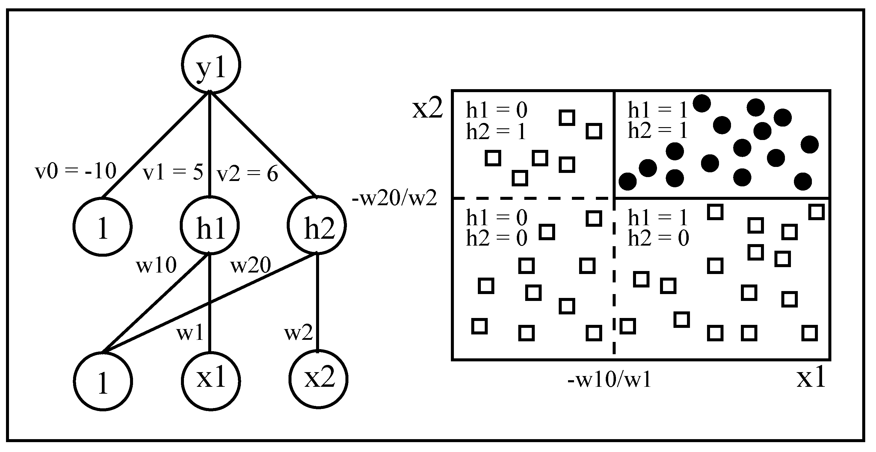
DIMLP differs from MLP in the connectivity between the input layer and the first hidden layer. Specifically, any hidden neuron receives only a connection from an input neuron and the bias neuron, as shown in Figure 3. This limited connectivity makes it possible to create axis-parallel byperplanes. Above the first hidden layer, neurons are fully connected.
4.1.1. DIMLP Architecture
In the first hidden layer the activation function is a staircase function that approximates the sigmoid function :
With and representing range bounds equal to and 5, the staircase function with q steps approximating is defined as:
Square brackets represent the integer part of a real value. Note that the step function is a particular case of the staircase function with only one step:
In all the other layers the activation function is a sigmoid. Note that the step/staircase activation function makes it possible to precisely locate possible discriminative hyperplanes. Specifically, in Figure 3 assuming two different classes, the first is being selected when (black circle) and the second with (white squares). Hence, two possible hyperplane splits are located in and , respectively. These splits are effective only when the two hidden neurons have an activation equal to one (upper right rectangle).
The training of a DIMLP network having step activation functions in the first hidden layer was performed by simulated annealing [44], since the gradient is undefined with step activation functions. When the number of steps approximates sufficiently well the sigmoid function, a modified back-propagation algorithm was used [17], the default value of q being equal to 50.
4.1.2. DIMLP Ensembles
We implemented DIMLP ensemble learning by bagging [45]. Specifically, from a training set containing p samples, each classifier in an ensemble includes p samples that have been drawn with replacement. Thus, each DIMLP network has many repeated/absent training samples. In this way, a certain diversity of each single network proves to be beneficial with respect to the whole ensemble of combined classifiers.
Rule extraction from ensembles can still be performed, since an ensemble of DIMLP networks can be viewed as a single DIMLP network with one more hidden layer. For this unique DIMLP network, weight values between sub-networks are equal to zero. Figure 4 illustrates three different kinds of DIMLP ensembles. Each “box” in this Figure is transparent, since it can be translated into symbolic rules. The ensemble resulting from different types of combinations is again transparent, since it is still a DIMLP network with one more layer of weights.
4.2. Quantized Support Vector Machines (QSVMs)
Functionally, SVMs can be viewed as feed-forward neural networks. Here, we focus on how an SVM is transformed into a QSVM, which is a DIMLP network with specific neuron activation functions. Hence, rules are generated by performing the DIMLP rule extraction algorithm. QSVM can be trained by SVM training algorithms, for which details are provided in [4], and in [46].
The classification decision function of an SVM model is given by
and b being real values, corresponding to the target values of the support vectors, and representing a kernel function with as the vector components of the support vectors. The sign function is
The following kernels are often used:
- Linear (dot product).
- Polynomial.
- Gaussian.
Specifically, for the dot and polynomial cases we have:
with for the dot kernel and for the polynomial kernel of third degree. The Gaussian kernel is:
with , a parameter.
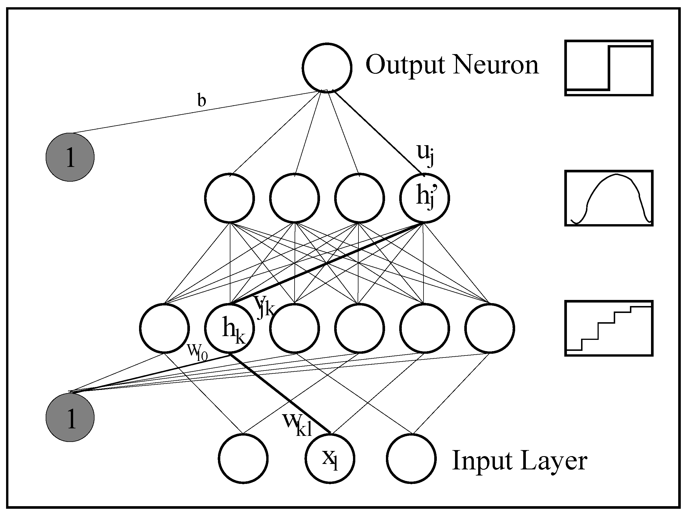
A Quantized Support Vector Machine (QSVM) is a DIMLP network with two hidden layers. A distinguishing feature of this model consists in the activation function of its second hidden layer. Specifically, it depends on the SVM kernel. As an example, Figure 5 depicts a QSVM with Gaussian kernel.
Likewise DIMLPs, the activation of the neurons in the first hidden layer is provided by a staircase function whose role is to carry out normalization of the inputs. This normalization is carried through weight values depending on the training data before the learning phase. Note that during training, these weights remain unchanged. Assuming that the number of neurons in the input layer is equal to the number of neurons in the first hidden layer, we define weight values as:
- , with as the standard deviation of input l;
- , with as the average on the training set of input l.
As stated above. the activation function in the second hidden layer depends on the SVM kernel. Hence, with a dot kernel it corresponds to the identity function, while with a polynomial kernel it is a cubic polynomial. All the weight values of the incoming connections into a neuron of the second hidden layer correspond to support vectors’ components. With respect to Figure 5, weight corresponds to the kth component of the jth support vector. Moreover, weight values between the second hidden layer and the output neuron corresponds to coefficients of Equation (6). Finally, the activation function of the output neuron is a sign function.
In this work we only use the dot kernel, since with an input layer having thousands of neurons the data is very likely to be well separated. Note that this kernel does not present parameters. To generate rules from a SVM network we build a QSVM network after a SVM network has been trained. Specifically, to build a QSVM network we perform the following steps:
- From the training set calculate for each input variable the average and the standard deviation.
- Define a partial QSVM network with an input layer and a second layer corresponding to the first hidden layer of the final QSVM network. The two layers are not fully connected, in order to precisely determine axis-parallel hyperplanes; weight values and bias values are fixed according to the average and standard deviations of inputs.
- From a training set T calculate a new training set , by forwarding all training samples of T from the input layer to the second layer of the partial QSVM network.
- With train a SVM network using a SVM training algorithm (in this work we use LS-SVM [42]).
- After learning, from the trained SVM network extract the support vectors (cf. Equation (6)) and define a new third layer of neurons corresponding to the second hidden layer of the final QSVM network; the incoming weights in this new layer are the support vectors’ components.
- From the SVM network extract the coefficients and the bias (cf. Equation (6)); they are used to define the weight values and the bias value between the second hidden layer and the output neuron of the final QSVM network.
5. Conclusions
This work illustrated transparent neural networks from which propositional rules were extracted to explain their classifications. Specifically, we showed several examples of rule antecedents involving the presence/absence of words relevant to sentiment polarity. Currently, rule extraction from connectionist models has not progressed as quickly as deep learning with Convolutional Neural Networks (CNNs). Even if we did not use CNNs, our main contribution is that we performed a rule extraction study in sentiment analysis that has been rarely carried out with shallow architectures. Specifically, we characterized the complexity of the knowledge embedded within models similar to SVMs and ensemble of MLPs.
It is likely that in the future rule extraction techniques will be applied to elucidate classification decisions of deep networks. This work can be viewed as an intermediate step towards rule extraction from CNNs. For that purpose, we will define DIMLP architectures aiming at emulating CNNs, by taking into account convolution and several particular activation functions related to CNNs. Propositional rules would be able to be generated, since the rule extraction algorithm used for DIMLPs can be applied to any number of hidden layers.
Author Contributions
Guido Bologna and Yoichi Hayashi conceived and designed the experiments; Guido Bologna performed the experiments; Guido Bologna and Yoichi Hayashi analyzed the data; Guido Bologna and Yoichi Hayashi wrote the paper.
Conflicts of Interest
The authors declare no conflict of interest.
Abbreviations
The following abbreviations are used in this manuscript:
| BOW | Bag Of Words |
| CNN | Convolutional Neural Network |
| DIMLP | Discretized Interpretable Multi Layer Perceptron |
| DIMLP-B | Discretized Interpretable Multi Layer Perceptron trained by Bagging |
| MLP | Multi Layer Perceptron |
| QSVM | Quantized Support Vector Machine |
| QSVM-D | Quantized Support Vector Machine with Dot kernel |
| SVM | Support Vector Machine |
References
- Andrews, R.; Diederich, J.; Tickle, A.B. Survey and critique of techniques for extracting rules from trained artificial neural networks. Knowl.-Based Syst. 1995, 8, 373–389. [Google Scholar] [CrossRef]
- Cambria, E.; Schuller, B.; Xia, Y.; Havasi, C. New avenues in opinion mining and sentiment analysis. IEEE Intell. Syst. 2013, 28, 15–21. [Google Scholar] [CrossRef]
- Dumais, S.T. Latent semantic analysis. Ann. Rev. Inf. Sci. Technol. 2004, 38, 188–230. [Google Scholar] [CrossRef]
- Vapnik, V.N.; Vapnik, V. Statistical Learning Theory; Wiley: New York, NY, USA, 1998; Volume 1. [Google Scholar]
- Harris, Z.S. Distributional structure. Word 1954, 10, 146–162. [Google Scholar] [CrossRef]
- Turney, P.D. Thumbs up or thumbs down?: Semantic orientation applied to unsupervised classification of reviews. In Proceedings of the 40th Annual Meeting on Association for Computational Linguistics, Philadelphia, PA, USA, 7–12 July 2002; pp. 417–424. [Google Scholar]
- Dey, L.; Haque, S.M. Opinion mining from noisy text data. Int. J. Doc. Anal. Recognit. 2009, 12, 205–226. [Google Scholar] [CrossRef]
- Cambria, E.; Hussain, A. Sentic Computing: Techniques, Tools, and Applications; Springer Science & Business Media: Berlin, Germany, 2012; Volume 2. [Google Scholar]
- Rosenthal, S.; Farra, N.; Nakov, P. SemEval-2017 task 4: Sentiment analysis in Twitter. In Proceedings of the 11th International Workshop on Semantic Evaluation (SemEval-2017), Vancouver, BC, Canada, 3–4 August 2017; pp. 502–518. [Google Scholar]
- Diederich, J.; Dillon, D. Sentiment recognition by rule extraction from support vector machines. In Proceedings of the CGAT 09 Proceedings: Computer Games, Multimedia and Allied Technology 09, Singapore, 11–12 May 2009. [Google Scholar]
- Bologna, G. Rule extraction from a multilayer perceptron with staircase activation functions. In Proceedings of the IEEE-INNS-ENNS International Joint Conference on Neural Networks, IJCNN 2000, Neural Computing: New Challenges and Perspectives for the New Millennium, Como, Italy, 27 July 2000; Volume 3, pp. 419–424. [Google Scholar]
- Bologna, G. A study on rule extraction from several combined neural networks. Int. J. Neural Syst. 2001, 11, 247–255. [Google Scholar] [CrossRef] [PubMed]
- Bologna, G.; Hayashi, Y. QSVM: A Support Vector Machine for rule extraction. In International Work-Conference on Artificial Neural Networks; Springer: Berlin, Germany, 2015; pp. 276–289. [Google Scholar]
- Freedman, D.A. Statistical Models: Theory and Practice; Cambridge University Press: New York, NY, USA, 2009. [Google Scholar]
- Russell, S.J.; Norvig, P.; Canny, J.F.; Malik, J.M.; Edwards, D.D. Artificial Intelligence: A Modern Approach; Prentice Hall: Upper Saddle River, NJ, USA, 2003; Volume 2. [Google Scholar]
- De Raedt, L. Logical and Relational Learning; Springer Science & Business Media: Berlin, Germany, 2008. [Google Scholar]
- Bologna, G. A model for single and multiple knowledge based networks. Artif. Intell. Med. 2003, 28, 141–163. [Google Scholar] [CrossRef]
- Zhou, Z.H.; Jiang, Y.; Chen, S.F. Extracting symbolic rules from trained neural network ensembles. Artif. Intell. Commun. 2003, 16, 3–16. [Google Scholar]
- Johansson, U. Obtaining Accurate and Comprehensible Data Mining Models: An Evolutionary Approach; Linköping University, Department of Computer and Information Science: Linköping, Sweden, 2007. [Google Scholar]
- Hara, A.; Hayashi, Y. Ensemble neural network rule extraction using Re-RX algorithm. In Proceedings of the 2012 International Joint Conference on Neural Networks (IJCNN), Brisbane, Australia, 10–15 June 2012; pp. 1–6. [Google Scholar]
- Hayashi, Y.; Sato, R.; Mitra, S. A new approach to three ensemble neural network rule extraction using recursive-rule extraction algorithm. In Proceedings of the 2013 International Joint Conference on Neural Networks (IJCNN), Dallas, TX, USA, 4–9 August 2013; pp. 1–7. [Google Scholar]
- Diederich, J. Rule Extraction From Support Vector Machines; Springer Science & Business Media: Berlin, Germany, 2008; Volume 80. [Google Scholar]
- Barakat, N.; Bradley, A.P. Rule extraction from support vector machines: A review. Neurocomputing 2010, 74, 178–190. [Google Scholar] [CrossRef]
- Barakat, N.; Diederich, J. Learning-based rule-extraction from support vector machines. In Proceedings of the 14th International Conference on Computer Theory and applications ICCTA’2004, Alexandria, Egypt, 28–30 September 2004. [Google Scholar]
- Torres, D.; Rocco, C. Extracting trees from trained SVM models using a TREPAN based approach. In Proceedings of the Fifth International Conference on Hybrid Intelligent Systems (HIS’05), Rio de Janeiro, Brazil, 6–9 November 2005; p. 6. [Google Scholar]
- Martens, D.; Baesens, B.; Van Gestel, T.; Vanthienen, J. Comprehensible credit scoring models using rule extraction from support vector machines. Eur. J. Oper. Res. 2007, 183, 1466–1476. [Google Scholar] [CrossRef]
- Martens, D.; Baesens, B.; Van Gestel, T. Decompositional rule extraction from support vector machines by active learning. IEEE Trans. Knowl. Data Eng. 2009, 21, 178–191. [Google Scholar] [CrossRef]
- Quinlan, J.R. C4.5: Programs for machine learning. morgan kaufmann publishers, inc., 1993. Mach. Learn. 1994, 16, 235–240. [Google Scholar]
- Barakat, N.; Diederich, J. Eclectic rule-extraction from support vector machines. Int. J. Comput. Intell. 2005, 2, 59–62. [Google Scholar]
- Barakat, N.H.; Bradley, A.P. Rule extraction from support vector machines: A sequential covering approach. IEEE Trans. Knowl. Data Eng. 2007, 19, 729–741. [Google Scholar] [CrossRef]
- Fu, X.; Ong, C.; Keerthi, S.; Hung, G.G.; Goh, L. Extracting the knowledge embedded in support vector machines. In Proceedings of the 2004 IEEE International Joint Conference on Neural Networks (IEEE Cat. No. 04CH37541), Budapest, Hungary, 25–29 July 2004; Volume 1, pp. 291–296. [Google Scholar]
- Núñez, H.; Angulo, C.; Català, A. Rule Extraction From Support Vector Machines. In Proceedings of the 10th European Symposium on Artificial Neural Networks (ESANN’02), Bruges, Belgium, 24–26 April 2002; pp. 107–112. [Google Scholar]
- Núñez, H.; Angulo, C.; Català, A. Rule-based learning systems for support vector machines. Neural Process. Lett. 2006, 24, 1–18. [Google Scholar] [CrossRef]
- Zhu, P.; Hu, Q. Rule extraction from support vector machines based on consistent region covering reduction. Knowl.-Based Syst. 2013, 42, 1–8. [Google Scholar] [CrossRef]
- De Fortuny, E.J.; Martens, D. Active learning-based pedagogical rule extraction. IEEE Trans. Neural Netw. Learn. Syst. 2015, 26, 2664–2677. [Google Scholar] [CrossRef] [PubMed]
- Ribeiro, M.T.; Singh, S.; Guestrin, C. Why should i trust you?: Explaining the predictions of any classifier. In Proceedings of the 22nd ACM SIGKDD International Conference on Knowledge Discovery and Data Mining, San Francisco, CA, USA, 13–17 August 2016; pp. 1135–1144. [Google Scholar]
- Weller, A. Challenges for Transparency. arXiv, 2017; arXiv:1708.01870. [Google Scholar]
- Henelius, A.; Puolamäki, K.; Ukkonen, A. Interpreting Classifiers through Attribute Interactions in Datasets. arXiv, 2017; arXiv:stat.ML/1707.07576. [Google Scholar]
- Rosenbaum, C.; Gao, T.; Klinger, T. e-QRAQ: A Multi-turn Reasoning Dataset and Simulator with Explanations. arXiv, 2017; arXiv:cs.LG/1708.01776. [Google Scholar]
- Pang, B.; Lee, L. Seeing stars: Exploiting class relationships for sentiment categorization with respect to rating scales. In Proceedings of the 43rd Annual Meeting on Association for Computational Linguistics, Ann Arbor, MI, USA, 25–30 June 2005; pp. 115–124. [Google Scholar]
- Pang, B.; Lee, L. A sentimental education: Sentiment analysis using subjectivity summarization based on minimum cuts. In Proceedings of the 42nd Annual Meeting on Association for Computational Linguistics, Barcelona, Spain, 21–26 July 2004; p. 271. [Google Scholar]
- Suykens, J.A.; Vandewalle, J. Least squares support vector machine classifiers. Neural Process. Lett. 1999, 9, 293–300. [Google Scholar] [CrossRef]
- Yin, Y.; Jin, Z. Dent ocument sentimclassification based on the word embedding. In Proceedings of the 4th International Conference on Mechatronics, Materials, Chemistry and Computer Engineering (ICMMCCE 2015), Xi’an, China, 12–13 December 2015; pp. 456–461. [Google Scholar]
- Bologna, G.; Pellegrini, C. Three medical examples in neural network rule extraction. Phys. Med. 1997, 13, 183–187. [Google Scholar]
- Breiman, L. Bagging predictors. Mach. Learn. 1996, 24, 123–140. [Google Scholar] [CrossRef]
- Burges, C.J. A tutorial on support vector machines for pattern recognition. Data Min. Knowl. Discov. 1998, 2, 121–167. [Google Scholar] [CrossRef]
Figure 1.
Plot of average complexity of rules versus average fidelity (RT-2k problem). Average complexity is the product of average number of rules by average number of antecedents per rule.
Figure 1.
Plot of average complexity of rules versus average fidelity (RT-2k problem). Average complexity is the product of average number of rules by average number of antecedents per rule.
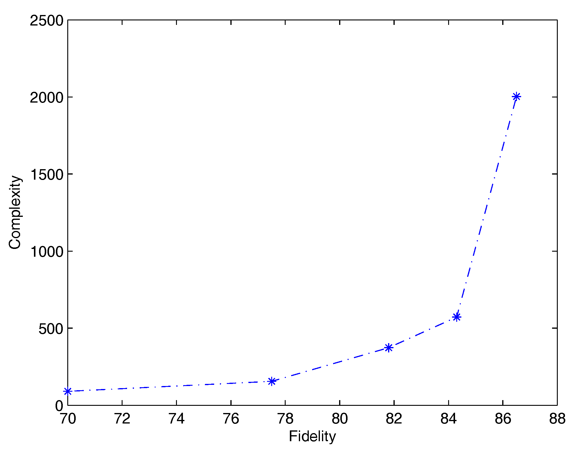
Figure 2.
Plot of average complexity of rules versus average fidelity (RT-s problem).
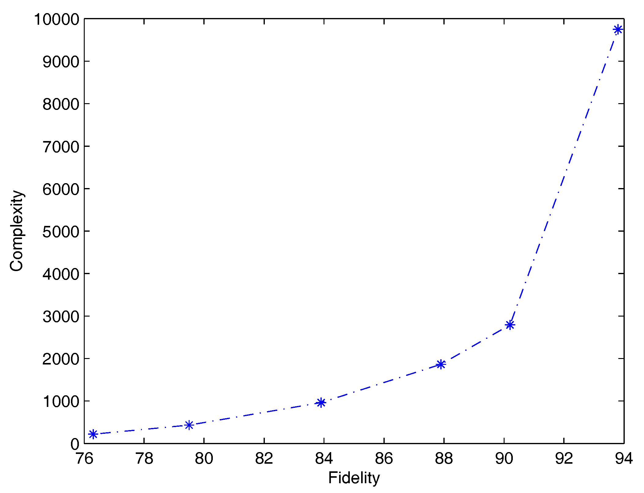
Figure 3.
A DIMLP network creating two discriminative hyperplanes. The activation function of neurons and is a step function, while for output neuron it is a sigmoid.
Figure 3.
A DIMLP network creating two discriminative hyperplanes. The activation function of neurons and is a step function, while for output neuron it is a sigmoid.

Figure 4.
Transparency of DIMLP ensembles by majority voting, linear combinations and non-linear combinations.
Figure 4.
Transparency of DIMLP ensembles by majority voting, linear combinations and non-linear combinations.
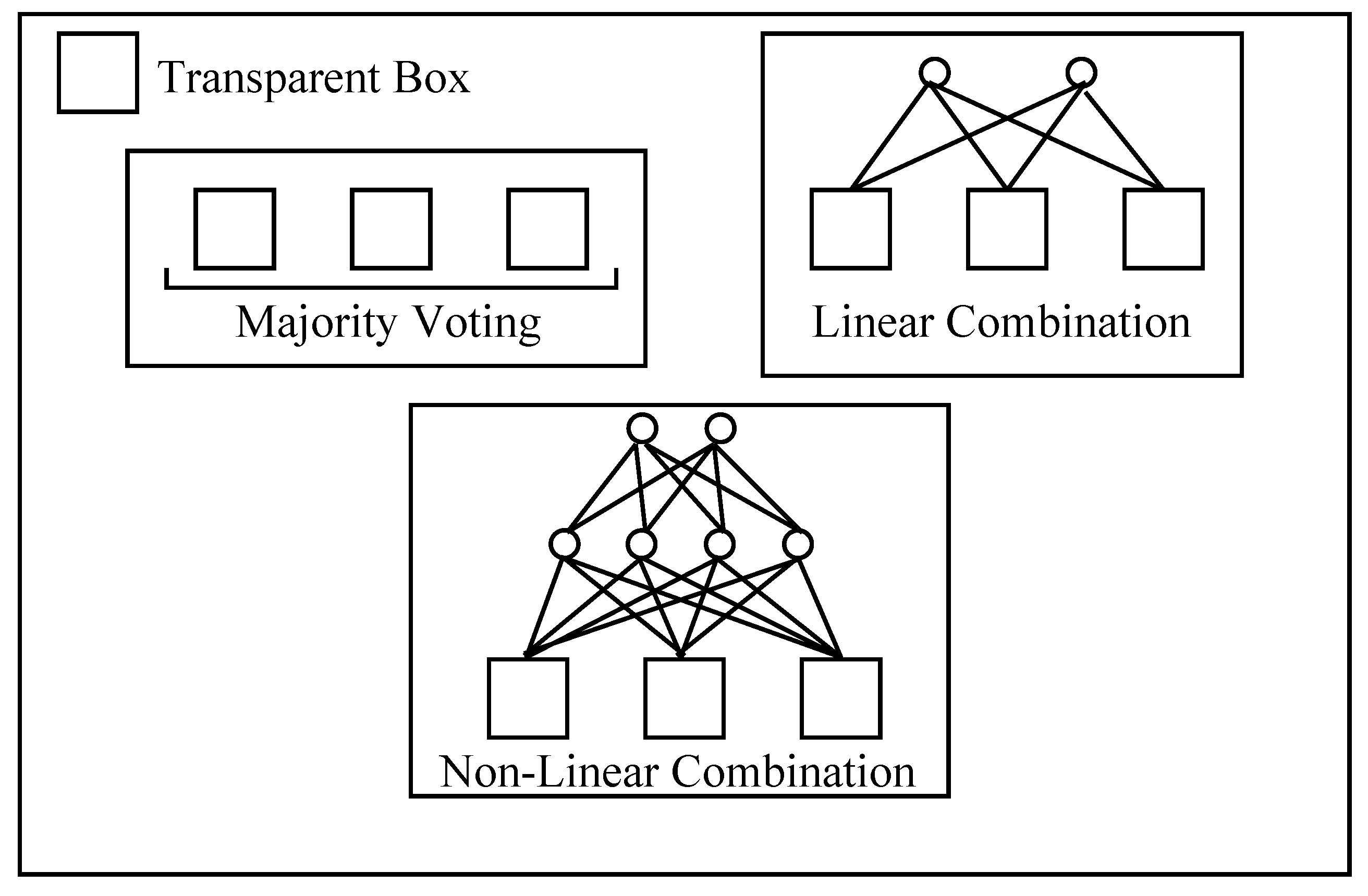
Figure 5.
A QSVM network with Gaussian kernel.

Table 1.
Datasets statistics.
| Dataset | (#Samples) | Maj. Class (%) | Avg. #Words | #Inputs |
|---|---|---|---|---|
| RT-2k | 2000 | 50 | 787 | 14,992 |
| RT-s | 10,662 | 50 | 21 | 4463 |
Table 2.
Average results obtained with the RT-2k dataset by DIMLP ensembles trained by bagging, QSVMs using the dot kernel and naive Bayes. Standard deviations are shown between round parentheses.
Table 2.
Average results obtained with the RT-2k dataset by DIMLP ensembles trained by bagging, QSVMs using the dot kernel and naive Bayes. Standard deviations are shown between round parentheses.
| Model | Acc. (%) | Rules Acc. (%) | Rules Acc. 2 (%) | Fidelity (%) | #Rules | #Ant. | #Def. (%) |
|---|---|---|---|---|---|---|---|
| DIMLP-B | 84.1 (2.8) | 80.3 (2.5) | 85.3 (2.6) | 91.2 (1.8) | 205.6 (27.0) | 8.1 (0.4) | 2.7 (0.9) |
| QSVM-D | 86.4 (1.7) | 78.3 (2.8) | 87.3 (1.7) | 86.5 (1.9) | 250.4 (16.8) | 8.0 (0.5) | 3.3 (1.2) |
| Naive Bayes | 59.0 (1.4) | – | – | – | – | – | – |
Table 3.
Required words in the top 20 rules generated from QSVMs (RT-2k dataset). For testing folds one to five, rules are ranked according to the number of activations with respect to the training set. Specifically, the ith row illustrates the required word of the ith rule, as well as rule polarity and the number of absent words. In bold are emphasized words that appear for the first time.
| Fold 1 | Fold 2 | Fold 3 | Fold 4 | Fold 5 |
|---|---|---|---|---|
| – (+), 73 | – (−), 44 | – (+), 52 | – (+), 52 | – (+), 47 |
| performances (+), 18 | – (+), 44 | worst (−), 14 | different (+), 18 | worst (−), 12 |
| especially (+), 18 | stupid (−), 9 | performances (+), 19 | others (+), 16 | looks (−), 25 |
| ridiculous (−), 7 | unfortunately (−), 17 | others (+), 16 | especially (+), 16 | ridiculous (−), 8 |
| others (+), 17 | others (+), 13 | boring (−), 10 | extremely (+), 11 | female (−), 12 |
| different (+), 18 | worst (−), 14 | memorable (+), 10 | effective (+), 14 | dull (−), 6 |
| boring (−), 13 | solid (+), 12 | ridiculous (−), 7 | awful (−), 8 | perfectly (+), 10 |
| stupid (−), 13 | supposed (−), 15 | perfectly (+), 10 | brilliant (+), 9 | above (+), 12 |
| true (+), 19 | wasted (−), 8 | stupid (−), 10 | overall (+), 12 | else (+), 21 |
| perfectly (+), 10 | hilarious (+), 16 | wasted (−), 7 | hilarious (+), 11 | none (−), 15 |
| wasted (−), 8 | annoying (−), 16 | awful (−), 6 | poor (−), 12 | idea (+), 23 |
| looks (−), 18 | anyone (+), 24 | guess (−), 14 | stupid (−), 12 | reason (+), 19 |
| awful (−), 8 | ridiculous (−), 6 | history (+), 13 | simple (+), 16 | bland (−), 4 |
| hilarious (+), 13 | america (+), 13 | material (−), 15 | wasted (−), 7 | supposed (−), 3 |
| unfortunately (−), 20 | dull (−), 8 | none (−), 13 | flaws (−), 10 | obvious (+), 15 |
| outstanding (+), 3 | neither (−), 17 | waste (−), 9 | absolutely (+), 11 | tries (+), 25 |
| lame (−), 4 | else (+), 25 | overall (+), 13 | lame (−), 6 | awful (−), 5 |
| pace (+), 11 | already (+), 18 | hilarious (+), 15 | reason (+), 31 | falls (+), 16 |
| wonderful (+), 12 | anyone (−), 4 | realistic (+), 7 | allows (+), 7 | color (+), 6 |
| reason (+), 23 | fails (−), 10 | mess (−), 10 | audiences (+), 13 | giving (+), 18 |
Table 4.
Required words in the top 20 rules generated from QSVMs (RT-2k dataset). For testing folds six to ten, rules are ranked according to the number of activations with respect to the training set.
Table 4.
Required words in the top 20 rules generated from QSVMs (RT-2k dataset). For testing folds six to ten, rules are ranked according to the number of activations with respect to the training set.
| Fold 6 | Fold 7 | Fold 8 | Fold 9 | Fold 10 |
|---|---|---|---|---|
| – (−), 36 | – (−), 44 | – (+), 40 | – (+), 50 | – (−), 41 |
| worst (−), 8 | performances (+), 17 | – (−), 40 | worst (−), 9 | performances (+), 16 |
| looks (−), 18 | stupid (−), 9 | – (−), 40 | unfortunately (−), 16 | worst (−), 12 |
| stupid (−), 6 | stupid (−), 9 | stupid (−), 9 | reason (+), 16 | boring (−), 16 |
| ridiculous (−), 6 | others (+), 16 | supposed (−), 13 | stupid (−), 8 | stupid (−), 9 |
| simple (+), 16 | perfectly (+), 9 | boring (−), 11 | awful (−), 6 | change (+), 8 |
| perfect (+), 14 | excellent (+), 10 | attempt (−), 19 | perfectly (+), 12 | brilliant (+), 11 |
| anyway (−), 12 | waste (−), 7 | perfect, (+), 17 | others (+), 17 | excellent (+), 10 |
| supposed (−) 11 | wasted (−), 6 | especially (+), 20 | supposed (−), 21 | memorable (+), 8 |
| different (+) 16 | memorable (+), 9 | worse (−), 12 | mess (−), 9 | supposed (−), 19 |
| enjoyable (+), 15 | worst (−), 10 | able (+), 17 | looks (−), 20 | none (−), 11 |
| extremely (+), 16 | hilarious (+), 10 | memorable (+), 10 | none (−), 12 | ridiculous (−), 7 |
| outstanding (+), 3 | wonderful (+), 13 | unfortunately (−), 14 | wasted (−), 8 | allows, (+), 6 |
| predictable (−), 12 | ridiculous (−), 9 | against (+), 17 | hilarious (+), 14 | wasted (−), 8 |
| definitely (+), 12 | different (+), 18 | ridiculous (−), 10 | supposed (−), 16 | terrific (+), 8 |
| true (−), 20 | begins (+), 19 | wasted (−), 6 | wasn’t (−), 12 | different (+) 18 |
| enjoyed (+), 13 | behind (−), 23 | excellent (+), 13 | attempt (−), 19 | powerful (+), 9 |
| sometimes (+), 16 | exactly (+), 22 | completely (+), 22 | dull (−), 8 | throughout (+), 17 |
| history (+), 14 | boring-worst (−), 3 | guess (−), 12 | overall (+), 11 | extremely (+), 14 |
| hilarious (+), 16 | terrific (+), 7 | boring-unfortunately (−), 2 | brilliant (+), 13 | sometimes (+), 13 |
Table 5.
Average results for the rules extracted from QSVMs by varying the number of training samples from 5% to 100% (RT-2k dataset).
Table 5.
Average results for the rules extracted from QSVMs by varying the number of training samples from 5% to 100% (RT-2k dataset).
| Model | Rules Acc. (%) | Rules Acc. 2 (%) | Fidelity (%) | #Rules | #Ant. | #Def. (%) |
|---|---|---|---|---|---|---|
| QSVM-D (5%) | 70.0 (4.6) | 87.0 (2.5) | 76.0 (4.9) | 32.3 (12.9) | 2.8 (0.6) | 9.4 (11.5) |
| QSVM-D (10%) | 71.7 (3.0) | 87.4 (2.0) | 77.5 (4.1) | 39.8 (4.3) | 3.9 (0.4) | 5.2 (3.7) |
| QSVM-D (20%) | 75.5 (3.8) | 87.8 (2.3) | 81.8 (4.0) | 71.9 (4.7) | 5.2 (0.4) | 5.9 (2.0) |
| QSVM-D (30%) | 77.7 (3.0) | 88.0 (2.0) | 84.3 (2.3) | 90.7 (9.1) | 5.8 (0.3) | 4.8 (1.1) |
| QSVM-D (100%) | 78.3 (2.8) | 87.3 (1.7) | 86.5 (1.9) | 250.4 (16.8) | 8.0 (0.5) | 3.3 (1.2) |
Table 6.
Average results obtained with the RT-s dataset by DIMLP ensembles trained by bagging, QSVMs using the dot kernel and naive Bayes. Standard deviations are given between round parentheses.
Table 6.
Average results obtained with the RT-s dataset by DIMLP ensembles trained by bagging, QSVMs using the dot kernel and naive Bayes. Standard deviations are given between round parentheses.
| Model | Acc. (%) | Rules Acc. (%) | Rules Acc. 2 (%) | Fidelity (%) | #Rules | #Ant. | #Def. (%) |
|---|---|---|---|---|---|---|---|
| DIMLP-B | 74.9 (1.4) | 73.4 (1.2) | 75.5 (1.3) | 94.8 (0.7) | 801.6 (21.2) | 11.4 (0.4) | 1.5 (0.3) |
| QSVM-D | 76.0 (1.4) | 74.3 (1.2) | 76.8 (1.4) | 93.8 (1.1) | 919.8 (30.6) | 10.6 (0.5) | 1.8 (0.6) |
| Naive Bayes | 75.9 (1.0) | – | – | – | – | – | – |
Table 7.
Required words in the top 20 rules generated from QSVMs (RT-s dataset). For testing folds one to five, rules are ranked according to the number of activations with respect to the training set. Specifically, the ith row illustrates the required word of the ith rule, as well as rule polarity and the number of absent words. In bold are emphasized words that appear for the first time.
| Fold 1 | Fold 2 | Fold 3 | Fold 4 | Fold 5 |
|---|---|---|---|---|
| – (−), 468 | – (−), 389 | – (−), 463 | – (+), 417 | – (−), 458 |
| movie (−), 141 | – (−), 387 | – (−), 470 | – (+), 146 | movie (−), 182 |
| but (−), 205 | but (−), 214 | – (−), 463 | with (+), 137 | movie (−), 122 |
| movie (−), 142 | this (−), 152 | movie (−), 134 | with (+), 136 | an (+), 123 |
| more (−), 131 | film (+), 139 | but (−), 160 | an (+), 133 | more (−), 92 |
| more (−), 121 | more (−), 116 | film (+), 141 | with (+), 154 | too (−), 39 |
| with (+), 107 | its (−), 188 | with (−), 219 | its (+), 135 | too (−), 35 |
| too (−), 36 | with (+), 140 | for (−), 134 | movie (−), 116 | so (−), 79 |
| for (−), 125 | like (−), 90 | too (−), 31 | but (−), 203 | you (+), 82 |
| an (+), 112 | movie (−), 130 | it’s (−), 153 | it’s (+), 117 | or (−), 85 |
| have (−), 96 | but (−), 144 | by (−), 104 | for (−), 166 | no (−), 40 |
| or (−), 69 | an (−), 190 | or (−), 78 | you (+), 97 | so (−), 75 |
| no (−), 35 | too (−), 30 | so (−), 61 | too (−), 42 | film (+), 117 |
| you (+), 70 | or (−), 69 | no (−), 52 | has (+), 99 | you (+), 81 |
| just (−), 54 | by (−), 111 | more (−), 78 | you (+), 88 | only (−), 52 |
| by (−), 97 | no (−), 42 | about (−), 87 | more (−), 88 | bad (−), 10 |
| on (−), 110 | all (−), 102 | only (−), 40 | by (+), 107 | its (+), 89 |
| film (+), 113 | bad (−), 7 | bad (−), 8 | no (−), 45 | it’s (+), 87 |
| so (−), 62 | only (−), 47 | you (+), 85 | so (−), 61 | or (−), 72 |
| only (−), 42 | bad (−), 7 | funny (+), 39 | or (−), 74 | funny (+), 37 |
Table 8.
Required words in the top 20 rules generated from QSVMs (RT-s dataset). For testing folds six to ten, rules are ranked according to the number of activations with respect to the training set.
Table 8.
Required words in the top 20 rules generated from QSVMs (RT-s dataset). For testing folds six to ten, rules are ranked according to the number of activations with respect to the training set.
| Fold 6 | Fold 7 | Fold 8 | Fold 9 | Fold 10 |
|---|---|---|---|---|
| – (−), 406 | – (−), 462 | – (+), 393 | – (+), 480 | – (−), 460 |
| with (−), 148 | movie (−), 149 | film (+), 148 | with (+), 139 | with (+), 122 |
| movie (−), 122 | with (+), 139 | an (+), 144 | an (+), 136 | this (−), 191 |
| with (+), 141 | film (+), 133 | with (+), 172 | film (+), 158 | movie (−), 142 |
| film (+), 129 | like (−), 96 | an (+), 127 | its (+), 140 | film (+), 132 |
| this (−), 190 | too (−), 29 | its (+), 140 | too (−), 36 | you (+), 97 |
| like (−), 96 | an (+), 121 | it’s (+), 130 | movie (−), 121 | like (−), 106 |
| too (−), 37 | more (−), 117 | with (+), 122 | this (+), 158 | more (−), 97 |
| movie (−), 130 | with (+), 119 | with (+), 139 | you (+), 93 | too (−), 35 |
| more (−), 92 | than (−), 88 | you (+), 92 | it’s (+), 118 | its (+), 99 |
| you (+), 78 | or (−), 135 | this (+), 123 | has (+), 102 | an (+), 97 |
| too (−), 31 | its (+), 89 | too (−), 38 | too (−), 29 | like (−), 77 |
| or (−), 78 | so (−), 57 | movie (−), 96 | but (−), 134 | so (−), 81 |
| no (−), 44 | you (+), 93 | too (−), 31 | more (−), 88 | or (−), 69 |
| by (−), 111 | one (+), 107 | best (+), 20 | no (−), 42 | no (−), 44 |
| an (+), 110 | by (−), 94 | on (+), 101 | or (−), 71 | no (−), 39 |
| bad (−), 10 | too (−), 23 | so (−), 72 | only (−), 50 | not (−), 101 |
| best (+), 20 | no (−), 39 | not (−), 107 | bad (−), 14 | just (−), 61 |
| you (+), 73 | bad (−), 8 | more (−), 68 | best (+), 23 | has (+), 94 |
| funny (+), 38 | only (−), 46 | good (+), 56 | their (+), 55 | bad (−), 8 |
Table 9.
Average results for the rules extracted from QSVMs by varying the number of training samples from 2.5% to 100% (RT-s dataset).
Table 9.
Average results for the rules extracted from QSVMs by varying the number of training samples from 2.5% to 100% (RT-s dataset).
| Model | Rules Acc. (%) | Rules Acc. 2 (%) | Fidelity (%) | #Rules | #Ant. | #Def. (%) |
|---|---|---|---|---|---|---|
| QSVM-D (2.5%) | 63.9 (2.7) | 76.1 (1.5) | 76.3 (4.1) | 84.6 (6.4) | 2.6 (0.3) | 7.8 (2.7) |
| QSVM-D (5%) | 67.0 (2.1) | 77.1 (1.7) | 79.5 (2.5) | 139.6 (14.5) | 3.1 (0.4) | 6.3 (2.8) |
| QSVM-D (10%) | 68.5 (1.3) | 76.5 (1.4) | 83.9 (0.9) | 229.3 (19.1) | 4.2 (0.4) | 4.7 (1.2) |
| QSVM-D (20%) | 71.0 (1.5) | 76.7 (1.4) | 87.9 (1.4) | 365.6 (18.6) | 5.1 (0.4) | 3.6 (0.9) |
| QSVM-D (30%) | 72.5 (1.5) | 76.9 (1.4) | 90.2 (1.2) | 465.4 (28.0) | 6.0 (0.4) | 3.6 (0.7) |
| QSVM-D (100%) | 74.3 (1.2) | 76.8 (1.4) | 93.8 (1.1) | 919.8 (30.6) | 10.6 (0.5) | 1.8 (0.6) |
© 2018 by the authors. Licensee MDPI, Basel, Switzerland. This article is an open access article distributed under the terms and conditions of the Creative Commons Attribution (CC BY) license (http://creativecommons.org/licenses/by/4.0/).
Share and Cite
MDPI and ACS Style
Bologna, G.; Hayashi, Y. A Rule Extraction Study from SVM on Sentiment Analysis. Big Data Cogn. Comput. 2018, 2, 6. https://doi.org/10.3390/bdcc2010006
AMA Style
Bologna G, Hayashi Y. A Rule Extraction Study from SVM on Sentiment Analysis. Big Data and Cognitive Computing. 2018; 2(1):6. https://doi.org/10.3390/bdcc2010006
Chicago/Turabian StyleBologna, Guido, and Yoichi Hayashi. 2018. "A Rule Extraction Study from SVM on Sentiment Analysis" Big Data and Cognitive Computing 2, no. 1: 6. https://doi.org/10.3390/bdcc2010006