2. Intermittency
The concept of intermittency, as introduced by Narasimha [
52], is commonly used in analysis and description of transitional boundary layer flows. The intermittency is the fraction of time that the flow is turbulent in a position in the boundary layer during the breakdown phase. It is zero in laminar flow and unity in fully turbulent flow. The start of transition is defined as the foremost position in the boundary layer where turbulent features become visible, which means that intermittency begins to deviate from zero. The end of transition is the foremost position where the full flow may be considered as turbulent, which means that intermittency approaches unity. So, the concepts of start and end of transition are only loosely defined.
In the very first phase of transition research, laminar and turbulent states were detected by the value of the wall shear stress. This implies that distinction can be made between a laminar and a turbulent value, which, for instance, is possible for zero pressure gradient mean steady flow over a flat plate. Further, this type of detection only allows the definition of intermittency at the wall and not in the interior of the boundary layer. Later on, the turbulent state during transition was detected by analysis of spectral properties or distribution properties of velocity component fluctuations. Turbulence scales are much smaller in the interior of a turbulent spot inside a transitional boundary layer than in the outer flow. Distinction can, e.g., be made by the magnitude of the first order or second order time derivative of the streamwise velocity component (Arnal and Julien [
53], Keller and Wang [
54]). Making the distinction requires the choice of a discriminator value. Another possibility is by analysis of distribution properties of velocity fluctuations, wall shear stress (a so-called quasi wall shear stress can be derived from hot film signals) or wall heat flux. Transition starts when the variance of the distribution begins to increase and the skewness begins to rise from a slightly negative value, typical for pre-transitional fluctuations, to a positive value. Intermittency is 50% at the position of maximum variance together with zero skewness. Transition goes towards the end when the variance returns to a low value and the skewness evolves from a negative value to a zero value (e.g., Gomes et al. [
55]). More advanced techniques use wavelet analysis of a hot film signal (Hughes and Walker [
56]) or wavelet analysis of velocity signals (Schobeiri et al. [
31]; Elsner et al. [
57]; Simoni et al. [
58]). With sufficiently refined techniques derived from distribution analysis or wavelet analysis, intermittency can also be determined in boundary layer flows perturbed by impinging wakes and distinction can be made between instability waves in laminar flow, propagating wave packages in laminar flow, developing turbulence within a turbulent spot and fully developed turbulence (e.g., Hughes and Walker [
56]).
The cited techniques allow distinguishing turbulent fluctuations during breakdown from laminar fluctuations in the pre-transitional boundary layer and from turbulence in the free stream. If distinction is made between turbulence due to breakdown and free-stream turbulence, intermittency evolves in wall-normal direction very sharply from zero at the wall to a maximum in wall vicinity, which typically forms a plateau up to 20% of the boundary layer thickness. Farther from the wall, it evolves gradually until a zero value in the free stream (e.g., Wang and Keller [
59,
60]).
Already in the pioneering period, it was observed by Narasimha [
52] that for mean steady flows, the streamwise evolution of the plateau value in the intermittency profile, as well as the values deduced from the wall shear stress, can be well described by:
The position
xt is the start of transition and
U is the velocity magnitude at the edge of the boundary layer. The description applies very well to natural transition. For bypass transition, there is some deviation for small values of intermittency (Gostelow et al. [
61]). The explanation is that start of breakdown is concentrated for natural transition, which means that turbulent spots all originate in a narrow space strip, while start of breakdown in bypass transition is distributed, which means that turbulent spots originate over a rather broad area.
The evolution law (1) can be applied to other forms of transition as well. It was found by Malkiel and Mayle [
62] that it describes very well transition in a separated shear layer under a mean steady oncoming free stream. They observed that intermittency is at maximum in the centre of the shear layer, which means on the line of maximum vorticity, and the maximum value follows very well the law (1). It was also found by Gostelow and Thomas [
63] that for wake-perturbed boundary layer flow, the law (1) describes well transition in separated state under low free-stream turbulence in between wake impacts. Furthermore, growth and spreading of turbulent spots induced by wake impact and those induced by a statistically steady free stream, are similar (Walker et al. [
64,
65]; Schobeiri et al. [
31]). Thus, the evolution law may also be used for describing transition induced by wakes in wake-perturbed flow.
The evolution law (1) was derived for steady flow transition in attached state from the geometric model on spot growth and spot propagation by Emmons [
66]. In this representation, spots are assumed to have a heart-shaped planform with a pointed leading edge. The leading edge travels at about 0.88 times the free-stream velocity and the trailing edge at about 0.5 times the free-stream velocity. The spots are supposed to grow in the planform view with an angle 2α. With these data, the probability can be expressed that the flow is turbulent on some position (
x,
y,
t) if the streamwise position of the birth of the spots and their production rate are imposed [
1]. The Narasimha-law follows for constant planform shape, constant spreading angle and constant proportionality factors of leading and tailing edge velocities. The dimensionless parameter σ depends on the planform shape, the spreading angle and the propagation velocities, while the factor
N is the spot production rate per unit distance in spanwise direction, with dimension (1/s)/m. These parameters can be obtained from correlations. For example, detailed correlations for α, σ, and
N were constructed by Gostelow et al. [
67] and Solomon et al. [
68]. The factor
Nσ/U in (1) has the dimension 1/m
2. In further discussions we use the spatial growth rate parameter of intermittency,
, with dimension 1/m. With this parameter, Equation (1) becomes:
or
The intermittency evolution law (1) may be written in dimensionless form by:
with
and
, where
is dimensionless.
Thus:
The following obvious relations are useful in further discussions.
From (2) follows:
With (3), this is:
From (3) follows also:
Thus, (6) may also be written as:
Typically, once intermittency has been determined experimentally, the linear law (7) is fitted to the results. By this fitting, the onset position (
xt) and growth rate (
βγ) are determined.
7. Conditionally Averaged Flow Equations
A transitional flow can be seen as a two-phase flow with turbulent and non-turbulent phases. It can be described by a homogeneous mixture model, with the intermittency the probability that the turbulent phase is present. Such a description requires conditional averaging of flow quantities and associated equations, where a conditioned average either means an average during a turbulent phase or during a non-turbulent phase. The technique was introduced by Libby [
105] and Dopazo [
106] for description of the intermittency at the outer edge of mixing layers and boundary layers. However, the description is general and can be applied to intermittency due to transition in the interior of boundary layers and free shear layers. It leads to conditionally averaged Navier-Stokes equations for the turbulent fraction and non-turbulent fractions of the flow, with interaction terms between these. These interaction terms need modelling and an equation for intermittency has to be added to the coupled sets of equations. Further, the turbulence in the turbulent phase has to be described by a turbulence model. A similar description can be added for the fluctuations in the non-turbulent phase, but this has not been done in techniques of this kind.
A conditionally averaged description of the flow goes well together with conditionally averaged experimental analysis of a transitional flow. Mean and fluctuating values are then defined during turbulent and non-turbulent phases as, e.g., for a the velocity component in the mean streamwise direction,
,
,
,
. The resulting Reynolds-stress is then
The contributions are due to the turbulent and non-turbulent (laminar) fluctuations and due to the interaction between the two phases.
From experimental results it can be derived that turbulence during a turbulent phase of a transitional flow can well be described by conventional turbulence models. Modelling of non-turbulent fluctuations requires an adapted model, but can be done using the same principles, as proved with LES by Lardeau et al. [
107].
Conditionally averaged flow equations and associated models for the interaction terms were constructed with boundary layer approximations by Vancoillie and Dick [
108] and applied to zero pressure gradient flat plate flows. The conditioned equations were combined with the Launder-Sharma low-Reynolds k-ε turbulence model and the intermittency was described by the Narasimha-law in streamwise direction, with imposed start and end of the transition. They showed that, ignoring contributions by laminar fluctuations, experimental results of fluctuation kinetic energy across a boundary layer can be well represented. A particular feature is that the fluctuation kinetic energy has two maxima, one close to the wall due to turbulence activity and one farther away from the wall due to interaction between the two phases.
The technique was extended by Steelant and Dick [
83] to the full Navier-Stokes equations. The conditioned equations were combined with the Yang-Shih low-Reynolds k-ε turbulence model and a streamwise version of the Narasimha-law in the form (6):
where
u is the magnitude of the local velocity,
s is a streamwise coordinate and the function
F(
s −
st) is a modified form of
in order to take distributed breakdown into account. The streamwise coordinate was derived through integration of
Start and growth of transition were determined with the formulae of Mayle (9), (19) and (20) for bypass transition, with slightly different coefficients and exponents. The observations were, again, that accurate prediction of the two peaks in the profiles of fluctuation kinetic energy across the boundary layer can be obtained.
The technique was generalised for analysis of a high-pressure turbine cascade with steady inflow [
109]. The generalisation consisted by the construction of a transport equation for the sum of the intermittency at the outer edge of a pre-transitional boundary layer due to impact by free-stream turbulent eddies (ζ) and the intermittency inside a boundary layer due to breakdown (
). We will detail this equation in the section on intermittency transport models.
The use of conditionally averaged equations is mainly motivated by fundamental rigour in the description of transitional flows, but it has not much meaning for engineering practise. A first drawback is that a double set of equations is necessary, which increases considerably the computational effort. However, a second aspect is that conditionally averaged description mainly helps in better prediction of profiles of fluctuation kinetic energy across the boundary layer but does not help much in improvement of predictions of shear stress. The large-scale interaction term (last term in Equation (29)) contributes approximately half-way the boundary layer and is the largest half-way the transition. Further, the contribution is much more significant for fluctuation kinetic energy than for shear stress, due to much less difference in the
v-components of velocity than in the
u-components. And even the differences in the
u-components are not as big as one would expect from pure laminar and pure turbulent velocity profiles, as demonstrated by Kuan and Wang [
110], due to the interaction between the two phases which is in the sense of attraction. This means that, technically, Equation (29) may be simplified into
and the approximation improves if global fluctuations are used in the turbulent term instead of conditioned averages. Further, the contribution of the non-turbulent part is only significant in the first stage of the development of transition and may be left out without much loss of accuracy. This way, a justification can be given to the usual practice of using intermittency technically as a parameter that evolves from zero to unity and that multiplies either the Reynolds stress obtained from a turbulence model or multiplies the production and destruction terms of the equation of turbulent kinetic energy in an eddy-viscosity turbulence model. A contribution by laminar fluctuations can then be added, but is not strictly necessary.
8. Streamwise Algebraic Transition Models
An algebraic transition model is an algebraic formula describing a quantity relevant for transition that is introduced in a turbulence model. Mostly, intermittency is prescribed and used as a multiplier factor of the eddy viscosity of a turbulence model or the production and destruction terms of the equation of turbulent kinetic energy. Traditionally, algebraic models prescribe the relevant parameter along streamlines with the formula of Narasimha or a similar formula. We call such models streamwise, because it is also possible to prescribe intermittency in wall-normal direction, as we discuss in a later section. Modern examples are the model by Fürst et al. [
111] and Kožulović and Lapworth [
112].
In the model of Fürst et al., intermittency is described by
where
γe is the intermittency of the free stream, which is 1 for a turbulent flow and 0 for a non-turbulent flow,
γi is the intermittency in the interior of the boundary layer, determined with the Narasimha-formula (4),
y is the distance to the wall and
δ995 is the 99.5% thickness of the boundary layer. The model is connected to the k-ω turbulence model version of Kok [
113]. The intermittency factor is a multiplier factor of the production term of the k-equation and a multiplier factor of the destruction term, but with a limiting value of 0.1. Onset of transition and growth of transition are obtained from correlations that are similar to those of Mayle. A particular aspect is that
Reθ is not derived from integral values but from the maximum value of the vorticity Reynolds number
. The ratio of the maximum of the vorticity Reynolds number to the momentum thickness Reynolds number is 2.193 for the Blasius boundary layer and this ratio depends on the shape of the boundary layer. The ratio is determined by a correlation that contains the pressure gradient, as a substitute for the shape factor. Determination of the maximum of thevorticity Reynolds number requires a search along lines perpendicular to a wall, but does not require integration operations. A structured grid is used in wall vicinity and grid lines in wall-normal direction are used as approximation for perpendicular lines. Similarly, grid lines in streamwise direction are used for the length coordinate in the Narasimha-formula. The model was applied to natural transition and bypass transition in steady mean flow and to wake-perturbed flow. For wake-perturbed flow, it functions exactly in the same way as for steady mean flow.
In the model of Kožulović and Lapworth, intermittency is described for natural transition and bypass transition by
where
Reθt and
Reθe are the values of
Reθ at start and end of transition, both determined from correlations derived from the AGS-correlation, involving turbulence intensity and pressure gradient. A structured grid is used in wall vicinity and grid lines in wall-normal direction are used as approximation for perpendicular lines. The momentum thickness Reynolds number is derived by integration along the wall-normal grid lines. By the form of the formula (34), a streamwise coordinate is not necessary. The intermittency is constant across the boundary layer. For separated flow, the intermittency
γS is started from zero and increased linearly as a function of streamwise distance in the zone of negative shear stress up to values above unity, but with a maximum of four, and decreased linearly in the zone of positive shear stress down to unity. The intermittency model is coupled to the one-equation Spalart-Allmaras turbulence model [
114]. The production term is multiplied with the maximum of
γNB and
γS and the destruction term with the same value, but with a lower limit of 0.02. The model was applied with good success to the T106A low-pressure turbine cascade with steady inflow at low and high turbulence levels (0.4% and 4%) and several values of the outlet Reynolds number. The model is non-local, but Kožulović and Lapworth [
112] describe how the computations can be organised such that there is not much efficiency penalisation in a parallel computation.
As an example of an older model, we take the model by Cho et al. [
115]. It is linked to a two-layer model with the standard k-ε model as outer model and the eddy viscosity in the inner zone derived from the k-equation and an algebraically prescribed length scale. The inner eddy viscosity is
The turbulent value of
A+, denoted by
, is dependent on the pressure gradient and is 25 for zero pressure gradient. For describing transition, the following formula is used:
Onset of transition is determined by the AGS-formula, used in a Lagrangian way. This means that a flow path is traced in the boundary layer edge vicinity and that that the correlation is used on such a path. The momentum thickness is obtained by integration along wall-normal grid lines of a structured grid.
A similar methodology was used by Michelassi et al. for analysis of stator-rotor interaction in a transonic turbine stage [
116]. They coupled the algebraic transition model to the standard k-ω turbulence model, with multiplication of the eddy-viscosity by the factor:
We close the discussion on streamwise algebraic models by a rather particular example, called prescribed unsteady intermittency method (PUIM). The technique was developed by Addison and Hodson [
117] and Schulte and Hodson [
118]. Unsteady probability patterns of intermittency on walls are determined by formulas derived from the geometric propagation theory of turbulent spots by Emmons. The spreading of spots and the calming after wake passage are taken into account. The technique requires boundary layer parameters and correlations for determining the positions of spot generation, their rate of production and their growth. The method can be coupled to any turbulence model, but it creates only intermittency values on surfaces and is limited to bypass transition. A particularity of the method is that calming after a wake passage is modelled by a calculated value of intermittency. This hinders the spontaneous relaxation generated by the Navier-Stokes equations, when a source for turbulence is switched off.
There are more streamwise algebraic transition models, but the ones described here can be seen as representative. They have some common features. They derive a parameter that is relevant for transition by an algebraic formula or sets of algebraic formulas and they use correlations for start and end of transition, which need the evaluation of boundary layer parameters, in particular the momentum thickness Reynolds number. They apply the correlations quite directly to the turbulence model and thus, in principle, produce a result that is as good as the correlations are. A limitation of these models is that they are fundamentally one-dimensional, which means that they describe transition along a streamline or a path-line. Their generalisation to a multidimensional and unsteady formulation is, however, quite simple, as explained in the next section on intermittency transport models.
9. Intermittency Transport Models
The algebraic intermittency law of Narasimha in the form (8) can serve as the basis for the definition of a transport equation of intermittency:
This equation can be generalised into:
where “
” is the local velocity vector,
U is the magnitude of the velocity at the edge of the boundary layer and
u is the magnitude of the local velocity. A further generalisation is
The function
Fonset switches from zero to unity at transition onset. The diffusion term is added to allow a profile of
γ across the boundary layer. Some of the factors in Equation (40) can easily be replaced by others. The factor
is approximately proportional to
in the range
γ = 0 to 0.35 and approximately proportional to
γ in the range
γ = 0.35 to 0.95. So, replacement of this term by
or
γ, or a combination of these factors is possible. The factor
has the same dimension as the shear rate magnitude
S or the rotation magnitude
Ω. For instance, Equation (40) may be replaced by:
The function
Flength is then a dimensionless function expressing the growth rate of the intermittency. The ratio of the factor
to
S or
Ω depends on the dimensionless thickness of the boundary layer and on the shape of the boundary layer. These dependencies have to be taken into account in the functions
Flength and
Fonset. However, this is not a practical problem. Correlations for onset of transition use
Reθ as dimensionless boundary layer thickness as a function of free-stream turbulence level and shape of the boundary layer described by the dimensionless pressure gradient. The supplementary dependencies can be taken into account by
Reθ and the dimensionless pressure gradient. A similar methodology can be used with a model where
Fonset is determined by sensors. So, the structure of Equation (41) can be recognised in many of the dynamic intermittency equations used for transition modelling. We illustrate this with examples that are representative for the local correlation-based, direct correlation-based and physics-based types.
9.1. The Local Correlation-Based γ-Reθ Model
The correlation-based model by Menter, Langtry et al. [
75,
76], later improved by Langtry and Menter [
77], is an intermittency model using only local variables. The transition model is combined with the SST k-ω turbulence model [
119]. Bypass transition in an attached boundary layer is derived from the transport equation:
Production and destruction terms are
The destruction term is used to preserve laminar flow prior to transition. The
Fturb function is defined such that the destruction term switches to zero outside a laminar boundary layer. Production is activated with the
Fonset function. The input to this function is the ratio of the shear rate Reynolds number
and a critical value of the momentum thickness Reynolds number
Reθc. The function becomes active if this ratio exceeds a threshold value which depends on the turbulence Reynolds number
. The critical value of the momentum thickness Reynolds number
Reθc comes from a correlation, but not in a direct way. The correlation defines a value of
Reθt for transition onset as a function of turbulence intensity and pressure gradient in the free stream. The correlation is used with local values, everywhere in the flow field. The values are then input of the source term of a transport equation which generates modified values of
Reθt, denoted by
:
The source term
Pθt enforces the free-stream values of
to be equal to
Reθt and is set to zero in boundary layers. The transport equation processes the value of
Reθt such that
inside a boundary layer is influenced by the properties of the flow prior to transition.
Reθc is then derived as a function of
.
In the original publications [
75,
76], the empirical functions
and
were not specified. Improved versions of these correlations were then published in [
77]. Meanwhile, some research groups had reconstructed these functions. Examples are Suluksna et al. [
120], Sørensen [
121] and Piotrowski et al. [
122].
For transition in a separated boundary layer at low free-stream turbulence, the production term in the k-equation is increased by an effective intermittency function γeff = max (γsep,γ), which is a multiplier factor of the production term in k-equation. The γeff function is set to a value larger than unity in the flow region in which the ratio ReS/(3.235Reθc), used as an indicator of a separated flow region, becomes larger than unity. This allows for fast transition to turbulence. The function switches off when the boundary layer reattaches and fully turbulent flow is recovered. So, this modification is not active in a fully developed turbulent boundary layer.
9.2. The Local Correlation-Based Transition Model of Menter et al.
The intermittency model by Menter et al. [
92] is a simplified version of the γ-Re
θ model by Menter, Langtry, et al. [
75,
76,
77]. The equation for
is not used in the new model and
Reθc is obtained from an algebraic formula. The general form of the γ-equation is the same as in the previous model (Equation (42)), but the production term was simplified into
Fonset is again a function of the shear rate Reynolds number and the critical Reynolds number,
Reθc. However, in the new model, the critical Reynolds number
Reθc is a direct function of the local turbulence intensity and the local pressure gradient. Local values of turbulence intensity and pressure gradient are approximated by functions of distance to the wall, specific dissipation rate and velocity gradient normal to the wall. So, determination of the mean velocity and pressure gradient at the boundary layer edge is avoided. Secondly, the functional relation between
Reθc and the local turbulence intensity and local pressure gradient (local correlations) was optimised by numerical experiments, starting from experimental correlations. So, there is no use anymore of experimental correlations as with the γ-Re
θ model. This way, the necessity to solve a transport equation for
is avoided.
Flength is a constant value. The destruction term in γ-equation was kept the same as in the previous model (Equation (44)).
For transition in a separated boundary layer at low free-stream turbulence, an additional production term was added to the k-equation. This term has as basic input the product of the shear rate magnitude and the vorticity magnitude. Its activity is limited to the separation flow region using ReS and γ.
9.3. A Local Intermittency Transport Model Employing Sensors
Ge et al. [
94] proposed the following transport equation for intermittency:
with the production term
The model is a further developed version of a model by Durbin [
93]. The
Fγ function triggers onset of bypass transition. The function depends on the vorticity Reynolds number,
ReΩ =
y2Ω/ν and
Tω, which is the product of the turbulence Reynolds number,
ReT =
k/(ων), and the ratio
Ω/ω. The destruction term reads
The destruction term ensures a laminar boundary layer prior to transition. The inputs of the functions,
Fturb and
Gγ are the vorticity Reynolds number,
ReΩ, and the turbulence Reynolds number,
ReT. The functions are designed such that the destruction term becomes zero outside a laminar boundary layer and in a fully turbulent boundary layer.
The transition in separated boundary layer is modelled with an effective intermittency with values above unity. It is a function of a sensor, composed by an approximation of the ratio of the second- and the first-order derivatives of streamwise velocity, which detects inflection, and distance to the wall. The sensor is an indicator of strong adverse pressure gradient flow and separation.
9.4. Our Own Non-Local Correlation-Based Transport Intermittency Model
The model consists of an equation for free-stream intermittency
ζ and one for near-wall intermittency
γ, combined with the SST k-ω turbulence model [
119]. The intermittency factor
γ represents the fraction of time during which near-wall velocity fluctuations, caused by transition, have a turbulent character. This intermittency factor tends to zero in the free stream. The free-stream factor
ζ expresses the intermittent behaviour of the turbulent eddies, coming from the free stream, impacting onto the boundary layer edge. Inside the boundary layer, these eddies are damped and the free-stream factor goes to zero near the wall. The free-stream factor is unity in the free stream. The turbulence weighting factor
τ is the sum of the two factors and is a multiplication factor of the production term of the k-equation. Both intermittency factors are modelled by a convection-diffusion-source equation.
Hereafter is a description of the latest version of the model. It is the version described in [
123], with one further small modification. The version of [
123] constitutes a repair of an earlier version [
124]. The major differences are better description of relaminarisation, replacement of the ad-hoc criterion for detection of strong wake impact in separated boundary layer state (free-stream turbulence level above 2.12% together with separated state) by a more rational criterion and use of the same criterion for strong wake impact in attached boundary layer state (there was no criterion for this type of transition in the earlier version). In the version described in [
123] the old criterion of 2.12% was left active. This is not necessary and it was later switched off.
The equation for free-stream intermittency is
The dissipation term (last term) realises a zero normal derivative of the free-stream factor near a wall. In combination with the boundary condition
ζ = 0, this leads to a zero free-stream factor across the major part of the boundary layer. The diffusion coefficient
μζ was determined to obtain the complement of a Klebanoff profile (one minus the formula of Klebanoff) for the free-stream factor prior to transition:
The equation and the expression of the viscosity coefficient were constructed by Steelant and Dick [
109] and used with conditionally averaged equations. They were modified somewhat and recalibrated by Pecnik et al. [
125] for globally averaged Navier-Stokes equations. The factors obtained by Pecnik et al. are C
1 = 3.5, C
2 = 15.
The equation for near-wall intermittency is
The role of the diffusion term is a gradual variation of
γ towards zero in the free flow. The boundary condition for
γ at the wall is a zero normal derivative. The source term in the equation determines the transition onset location and the growth of the intermittency in the transition zone. The ingredients are a starting function
FS, a growth factor
βγ and a velocity scale
Uγ. Without diffusion term,
FS = 1 and
Uγ equal to the local velocity magnitude, the equation reproduces the Narashima-law. In a laminar flow,
FS is set to zero. The intermittency equation then generates
γ equal to zero.
FS is set to unity at start of transition for every type of transition, using onset correlations and the corresponding growth factors. The velocity scale
Uγ is set to the local velocity magnitude for attached flow transition and to the boundary layer edge velocity magnitude for separated flow transition. This way is approximately expressed that in separated flow the instability evolves along the inflection line. If, after activation of transition, no onset criteria are satisfied anymore,
FS is set to zero. The production term of the
γ-equation then becomes zero and near-wall intermittency is convected out. This way, calming is obtained as a result of the Navier-Stokes equations, after a wake passage.
A particular aspect of this model is the explicit equation for the impact of the free-stream turbulence on the edge of the boundary layer. In the other models discussed above, there is only one equation for intermittency. The boundary conditions for this intermittency are then a unit value in the free stream and zero normal derivative at a wall. With the present model, a unique equation can be obtained by adding the two Equations (50) and (52) into an equation for
τ =
ζ + γ, by writing the diffusion term as in Equation (50). This was actually done this way by Steelant and Dick [
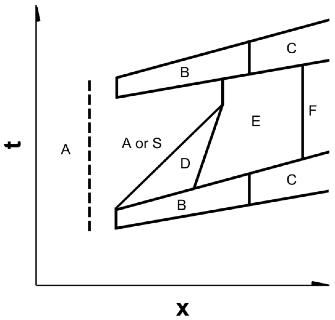
109] for applications to steady flows. In a steady flow, the impact on the pre-transitional layer is upstream of the breakdown such that the equations can be added up. However, in wake-induced transition, breakdown by turbulence in a wake can be upstream of impact of free-stream turbulence to the boundary layer edge, as illustrated in
Figure 3. It is thus more accurate to use separate equations. Of course, this increases the computational effort.
The onset criteria (9) and (11) for steady transition in attached boundary layer state and in separated boundary layer state (17) with corresponding growth rate factors (19) and (23) are used in steady flow and for quasi-steady transition in wake-perturbed flow. These criteria are always verified and the most critical one determines the onset. With the criteria, the onset function is set to unity across the whole boundary layer on the wall-normal grid lines. A criterion for strong wake impact is added by comparing two time scales: the time scale of the temporal growth of the turbulent kinetic energy Tstart = k/(dk/dt) of the oncoming turbulence impact of a wake and the dissipation time scale of the turbulence Tturb = k/ε = 1/(β*ω). Both time scales are calculated at the boundary layer edge. An impact is considered as strong if Tstart < Tturb. For an attached boundary layer, the intermittency growth rate is then switched from slow growth (19) to fast growth (23). For a separated boundary layer, onset of transition is then set as immediate and the fast growth rate (23) is applied. The modifications for strong wake impact are switched off when the time scale criterion is not satisfied anymore.
9.5. Other Transport Models
There exist many more intermittency transport models than described here, but the main principles are covered by the examples discussed. Savill [
126] was the first to use an intermittency transport equation combined with a turbulence model. He used the equation by Cho and Chung [
127] designed for description of intermittency at the edge of a turbulent shear layer and a surrounding laminar flow. This intermittency equation is meant to be physical and does not involve correlations. He showed significant improvement of predictions of bypass transition by adding the intermittency equation to the low-Reynolds form of a Reynolds-stress model. The intermittency equation was slightly modified by Vicedo et al. [
128] and applied to a low-Reynolds k-ε model. It was combined with a turbulence indicator function which switches off the production and destruction terms of the turbulence model if separation is detected and switches these again on if the Mayle-criterion for start of transition in separated state (17) is satisfied. Suzen, Huang et al. [
74,
129,
130] used an intermittency equation which is a combination of the equations of Steelant and Dick [
83] and Cho and Chung [
127]. In their model, the intermittency is a multiplier factor of the eddy viscosity by the SST k-ω turbulence model and is used in the Navier-Stokes equations, but the turbulence equations are not modified. They constructed own correlations for onset of bypass transition in an attached boundary layer and for onset of separation-induced transition. A remarkable feature is that the growth rate correlation of Mayle (19) is used for all types of transition, but with a coefficient enlarged to 18. They obtained good results for transition in attached boundary layer state and in separated boundary layer state on a low-pressure turbine cascade with steady inflow, but the validation of their model for wake-induced transition was very limited. A last model that we mention is by Wang et al. [
131]. The intermittency equation has the structure of Equation (41), but with
instead of
and onset of transition is given by a sensor based on the turbulent kinetic energy and the ratio of the magnitude of the gradient of the turbulent kinetic energy to the magnitude of the gradient of the mean flow kinetic energy.
11. A Wall-Normal Algebraic Transition Model
In this section, we describe our own algebraic transition model [
88]. As in the other sections, we discuss only the fundamental ingredients. The model is a further developed version of an earlier model [
135]. It is combined with the newest version of the k-ω model by Wilcox [
136].
The transport equations for turbulent kinetic energy and specific dissipation rate are
There are three modifications in the production terms. In the original model, production of turbulent kinetic energy by turbulent shear is
, with
νT the eddy viscosity and
S the shear rate magnitude. Firstly, this production term is written as
, where
νs is the small-scale eddy viscosity, which is part of the full eddy viscosity
νT. Secondly, in the k-equation, the production term
Pk is multiplied with an intermittency factor γ , which is zero in laminar flow and unity in turbulent flow. Thirdly, the term
(1 − γ)Psep is added to the production term of the k-equation. This term expresses turbulence production by instability and breakdown of a laminar free shear layer in a low turbulence level background flow.
The turbulent kinetic energy
k is split, based on the laminar-fluctuation kinetic energy transition model by Walters and Cokljat [
85], into a small-scale part
ks and a large-scale part
kℓ by
The splitting by the factor
fSS (Equation (27)) expresses the shear-sheltering effect in a pre-transitional boundary layer, by which is meant a boundary layer with a large near-wall laminar part. The effect means that small-scale disturbances in the turbulent flow near to the laminar part of the layer are damped by the vicinity of the laminar shear flow. Only large-scale disturbances penetrate deeply into the laminar layer, but these do not contribute to turbulence production by shear and induce the streaks. In the model, the restriction of the turbulence production by turbulent shear to small-scale fluctuations is expressed by replacing the full eddy viscosity by a small-scale eddy viscosity in the production term for turbulent shear.
The eddy viscosity associated to small scales is calculated in the same way as the eddy viscosity of the original turbulence model [
136] by replacing k by
ks:
The constant
a1 is set to 0.3 and
Clim = 7/8, which are the standard values. The large-scale eddy viscosity, is, similarly defined with
kℓ:
The constant
a2 is set to 0.6, which is larger than the standard value 0.3. The resulting eddy viscosity, used in the Navier-Stokes equations, is
νT = νs + νℓ. The reason for the enlarged value of
a2 with respect to
a1 is earlier transition due to increased instability of a laminar flow perturbed by streaks under an adverse pressure gradient, as observed by Zaki and Durbin [
137]. We express this effect by a somewhat higher eddy viscosity associated to large-scale perturbations, and consequently a somewhat higher turbulent stress, which becomes mainly active in adverse pressure gradient flow.
The intermittency function
γ determines when a flow region is laminar or turbulent. The free stream is turbulent. Thus,
γ is set to unity in the free stream. At a wall, the flow is laminar. Hence,
γ is set to zero there.
γ is prescribed algebraically as a function of the distance to the wall by:
were
Aγ is a constant. The non-dimensional representation of the distance to the wall is
. The intermittency
γ is zero for
Rey ≤
Aγ, unity for
Rey ≤ 2
Aγ and it varies linearly in between. In the section on sensors, we explained that
is an estimator of the normalised shear stress. The role of the intermittency function is modelling flow breakdown into turbulence for bypass transition when
, reaches a critical value.
Turbulence production due to breakdown of a laminar separated boundary layer at low free-stream turbulence level is modelled by the term (1 −
γ)
Psep in the k-equation (Equation (68)). For
Psep, we adopted a term with the same purpose in the newest intermittency-transport transition model by Menter et al. [
92]:
with
The sensor is the shear rate Reynolds number
ReS, as in the model by Menter et al. [
92], but
Psep is simplified.
12. Tests of Transition Models for Steady Inflow
In this section, we review some tests reported in the literature on transition prediction in attached boundary layer state and in separated boundary layer state for steady inflow.
Cutrone et al. [
138,
139] tested some models for steady flow bypass transition in attached boundary layer state and for steady flow transition in separated state. The models tested for bypass transition were the dynamic intermittency model of Steelant and Dick [
83], but applied to Reynolds-averaged equations, the dynamic intermittency model of Suzen and Huang [
74] and the laminar fluctuation kinetic energy model of Walters and Leylek [
87]. The intermittency models were combined with the correlation of Suzen and Huang [
74] for onset of transition and the correlation for growth of transition by Mayle (Equation (19)), but with the coefficient enlarged to 18. Because the same correlations were used, the models by Suzen and Huang and by Steelant and Dick become almost identical. This statement applies with good approximation to all direct correlation-based intermittency transport models, because these are essentially a technical means to impose the correlations. The test cases for bypass transition were the T3 flat plate flows of ERCOFTAC [
140] and a high-pressure turbine cascade. All models perform quite well for these cases. This is not fully surprising because such cases are used in the tuning of models.
For separated flow transition, they verified the model by Suzen and Huang and the model by Walters and Leylek for several levels of turbulence and several Reynolds numbers on the T3L case of ERCOFTAC [
140]. The Suzen and Huang model was combined with the criterion for onset of transition of long separation bubbles by Mayle (Equation (16)). The results of the k-k
L-ω model are always good. The separation bubble predicted by the Suzen and Huang model is mostly too large. We consider these tests as not conclusive for the direct correlation-based intermittency transport model of Suzen and Huang, because the transition onset correlation used seems not appropriate. The Walters and Leylek model was also tested on a cascade of T106 low-pressure turbine blades for several levels of inflow turbulence and two exit Reynolds numbers (500 × 10
3 and 1.1 × 10
6). The flow at the suction side was separated for all cases, except for the highest Reynolds number combined with turbulence levels above 3%. The predictions with separated flow are very good for the lowest Reynolds, less accurate for the high Reynolds number. However, the model predicts correctly attached flow transition. The model of Walters and Leylek was further employed for simulation of the three-dimensional flow in a cascade with T106 blades. Good correspondence was observed between measured and computed loss coefficients.
Choudry et al. [
141] studied the 2D steady flow over a NACA 0021 aerofoil at various angles of attack using the laminar kinetic energy model by Walters and Cokljat [
85] and the γ-Re
θ model by Langtry and Menter [
77]. The predictive qualities of the models were verified for short and long separation bubbles. Both models capture quite well both the lift and drag coefficient at small angle of attack (up to 12°), but the Walters and Cokljat model was found superior to the γ-Re
θ model for prediction of the drag coefficient at high angle of attack (up to 20°). At high angle of attack, the reattachment length by the γ-Re
θ model is much too short compared to the experiment owing to a too strong turbulence production at the leading edge of the separation bubble.
Sanders et al. [
142,
143] verified the laminar fluctuation kinetic energy model of Walters and Leylek [
87] for steady inflow of a lightly loaded LP-turbine cascade for inlet Reynolds numbers from 15 × 10
3 to 100 × 10
3 and inlet turbulence level of 1% and for steady inflow of a highly loaded low-pressure turbine cascade for inlet Reynolds numbers from 25 × 10
3 to 100 × 10
3 and inlet turbulence level of 0.6% using 2D and 3D URANS techniques. With the lightly loaded cascade, the flow at the suction side was separated for the lower Reynolds numbers and attached for the higher Reynolds numbers. The flow was attached at the pressure side. With the highly loaded cascade, the flow was separated both at the pressure side and the suction side and strongly unsteady at the suction side. The results compare quite well with experimental data, but the roll-up vortices at the trailing edge of the suction side stay largely two-dimensional. This means that the physical three-dimensional breakdown mechanism is not reproduced.
Marty [
144] tested the γ-Re
θ model of Langtry and Menter [
77] for separation-induced transition on the high-lift T106C low-pressure turbine cascade for exit Reynolds numbers 80 × 10
3, 140 × 10
3 and 250 × 10
3 and free-stream turbulence level in the leading-edge plane of 0.9%. The boundary layer was separated at the suction side and attached at the pressure side. The predictions are qualitatively correct, but for
Re = 80 × 10
3, the separation point is somewhat upstream of the experimental one and for
Re = 140 × 10
3 the reattachment point is somewhat upstream of the experimental one. For
Re = 250 × 10
3, predictions are very good.
Fürst et al. [
111] tested their own algebraic intermittency model and the laminar kinetic energy model by Walters and Cokljat [
85] for bypass transition in steady flows over flat plates, flow over two NACA 0012 aerofoils in a tandem configuration at
Re = 200 × 10
3, 400 × 10
3 and 600 × 10
3 and free-stream turbulence level 0.3% (zero angle of attack) and flow through a high-pressure turbine cascade for exit Reynolds number 590 × 10
3 and free-stream turbulence level at inlet to the cascade
Tu = 1.5%. The algebraic and laminar kinetic energy models show quite good correspondence between measured and computed skin friction coefficient for the flow over the aerofoils. The results are also good for bypass transition on the suction side of the turbine blade.
Pacciani at al. [
91] tested the γ-Re
θ model by Langtry and Menter [
77] and their own k-k
L-ω-I model for transition in separated state on the suction side of blades in a very-high-lift front-loaded (T108) and a very-high-lift aft-loaded (T106C) low-pressure turbine cascade. They tested the γ-Re
θ model with several closure functions from the literature. The turbulence intensity at inflow was always 0.8%. The exit Reynolds number was varied over a wide range. With the T108, the separation bubble by the γ-Re
θ model is too large and the building up of shear stress after reattachment is much too slow for all sets of closure functions. The value of the shear stress is too low in the breakdown region of the bubble. The k-k
L-ω-I model produces good results. With the T106C, all results are quite good, but the k-k
L-ω-I model performs somewhat better than the γ-Re
θ models. These tests illustrate that the γ-Re
θ model is primarily meant for bypass transition and that the extension to transition in separated state is less reliable. For the k-k
L-ω-I model it is the inverse. This model is primarily designed for transition in separated state and is extended for transition in attached boundary layer state.
From the reported tests with steady inflow, one can conclude that transition models, in principle, predict quite well for steady inflow, although not perfect, of course. Not all combinations of models and flow patterns have been tested. In particular tests on strongly separated flows are limited. We think that we can conclude from the literature that models that have been designed for bypass transition function well for this type of transition. This applies to direct correlation-based models, the local correlation-based γ-Re
θ model of Menter, Langtry et al. [
75,
76,
77], and the laminar kinetic energy models of Walters and Leylek [
87] and Walters and Cokljat [
85]. For transition in separated state, the intermittency models are less reliable, in particular for flows with very large separation zones. Direct correlation-based models impose, in principle, the results of correlations, but these are not fully reliable for separated flows. The local correlation-based γ-Re
θ model has a rather simple model ingredient for separated flows, which, very likely, cannot be fully universal. That predictions for strong separation are not very good can thus be believed. Remarkably, the models of Walters et al. seem to function quite well for separated flows, although these models have no specific ingredients for separated flows and use the same methodology as for attached flows. This is probably the result of model calibration on separated boundary layer flows with steady inflow, because Walters and Cokljat [
85] demonstrate good performance for separated boundary layer flow over the S809 aerofoil for angles of attack up to 15°. The k-k
L-ω models of Pacciani et al. were designed for flows with separation and perform very well for such cases, but these models have no specific ingredients for bypass transition in attached flows.
13. Tests of Transition Models for Wake-Perturbed Inflow
In this section, we review some tests reported in the literature and we report on an own test about wake-induced transition on the suction side of a turbine blade.
Wake-induced transition is challenging for transition models, because, usually, such cases are not considered during tuning and developers hope that tuning for steady inflow is sufficient. We report on one test on wake-induced transition by Pacciani et al. [
91] on the suction side of the T106A blade and two tests on wake-induced transition by Piotrowski et al. [
122,
145] on the suction side of the N3-60 blade. Later, we illustrate the predictive qualities of four transition models for wake-induced transition on the suction side of the N3-60 blade.
Pacciani at al. [
91] tested the γ-Re
θ model by Langtry and Menter [
77] and their own k-k
L-ω-I model for wake-induced transition on the suction side of the T106A low-pressure turbine blade for background turbulence level
Tu = 4%. In between wake impacts, the boundary layer at the suction side is prone to separation, but not separated. Boundary layer transition is thus of bypass type or by strong wake impact. Pacciani et al. report that the
Fθt function in the
equation of the γ-Re
θ model may erroneously switch to unity outside boundary layer regions and suggest a repair of the sensor for boundary layer presence. Both models predict a somewhat too early transition under wake-impact. In between wakes the relaxation towards the separated flow is better captured with the k-k
L-ω-I model than with the γ-Re
θ model. However, overall, both models reproduce quite well the major features of the boundary layer unsteady evolutions.
The N3-60 cascade has blades with the profile of that of a stator vane in the high-pressure part of a steam turbine. The cascade was experimentally analysed by Zarzycki and Elsner [
146]. Geometric characteristics of the N3-60 cascade are: blade chord 300 mm, axial blade chord 203.65 mm, blade pitch 240 mm. Full details on the blade geometry are specified in [
123]. In the experiments, the wake generator was a wheel of pitch diameter
Dp = 1950 mm with cylindrical bars rotating in a plane perpendicular to the flow direction. The bars were spaced by
bs = 204 mm on the pitch circle. The axial distance between the bars and the leading edge of the blades was 0.344 of the axial blade chord. The frequency of the incoming wakes was
fd = 59 Hz, with an inflow velocity
U0 = 10 m/s, resulting in the reduced frequency:
St =
fd·bs/U0 = 1.22. The exit velocity was
U1 = 30 m/s, which corresponds to an exit Reynolds number of 600 × 10
3. The free-stream turbulence intensity Tu was controlled with a movable grid upstream of the cascade entrance. Data were recorded for bar diameter 4 mm with inflow turbulence level
Tu = 0.4% and for bar diameter 6 mm with inflow turbulence level
Tu = 3%. This cascade is very useful because detailed experimental data are available on the evolution of the fluctuating streamwise velocity component (parallel to the surface) above the suction side of the blade. This is crucial for proper validation of transition models. The boundary layer is attached at the suction side for both cases, but is prone to separation for the low inflow turbulence level.
In [
145], Piotrowski et al. tested the PUIM [
118] and the dynamic intermittency model of Lodefier and Dick [
124] on the N3-60 for background inflow turbulence level 3%. PUIM generates quite good results, except that the relaxation to laminar state after the wake passage is incomplete, which means that the boundary layer does not return to fully laminar state, as it is the case in the experiments. We attribute this deficiency to the algebraic prescription of intermittency during calming. We are convinced that calming is better described by setting
γ fast to zero and let the relaxation be the result of the reaction of the Navier-Stokes equations. With the dynamic intermittency model, the start of transition under the wake impact is too slow, but the predictions of the time-varying intermittency and shape factor are good, but with a time lag of about 15% of the wake impact period. This deficiency was repaired in a later version by Kubacki et al. [
123] by the introduction of an onset for strong wake impact, as described before. In [
122], Piotrowski et al. tested the PUIM [
118], the dynamic intermittency model of Lodefier and Dick [
124] and the γ-Re
θ model, but combined with their own correlations, on the N3-60 for background inflow turbulence level 0.4%. All models produce very good predictions of the time-varying intermittency and momentum thickness, but with a time lag of about 15% of the wake impact with respect to the experiments.
Hereafter, we illustrate an application of four k-ω based transition models to wake-induced transition on the suction side of the N3-60 blade. The models tested are: the laminar fluctuation kinetic energy model (k-k
L-ω) model by Walters and Cokljat [
85], our own correlation-based dynamic intermittency model [
123], which is non-local because it uses boundary layer integral quantities, the local correlation-based dynamic intermittency transition model by Menter et al. [
92], and our own wall-normal (local) algebraic intermittency model [
88]. We use the following abbreviated names for the intermittency types: direct intermittency model, local intermittency model and algebraic intermittency model. By the term direct, we mean that the correlations are directly imposed to the intermittency equation, while in the local model this is done in an indirect way by a sensor of the boundary layer momentum thickness. We denote the laminar fluctuation kinetic energy model by k-k
L-ω model. The model by Menter et al. was used without activation of the Kato-Launder limiter since activation of this term caused very strong damping of the wake turbulence at the leading edge of the blade. The models are combined with k-ω turbulence models, but the model versions are not always the same. The k-k
L-ω model uses the version by Walters and Cokljat, which is near to the standard k-ω model [
133]. The direct and local intermittency models use the SST version [
119] and the algebraic intermittency model uses the newest version by Wilcox [
136]. The simulations were done with the ANSYS-Fluent package. The k-k
L-ω model and the local intermittency model were programmed by the developers of the package. We programmed the direct and algebraic intermittency models and the linked k-ω turbulence models with “User Defined Functions” (UDF).
The inlet to the computational domain was placed at 0.17 times the axial chord length upstream of the leading-edge plane. This position is about half-way between the moving bar system of the experiments and the leading edges of the blades. The effect of the moving bars was superimposed on the flow obtained from a steady calculation. The bar pitch was increased to 240 mm to be equal to the blade pitch in the calculation. The bar velocity was adjusted so that the reduced frequency (
St) of the impacting wakes is unchanged; 800-time steps were used per wake period. As shown by Piotrowski et al. [
145], this number of time steps is sufficient for capturing the wake characteristics. Self-similar profiles for velocity and turbulent kinetic energy were imposed at the inlet:
In the above expressions,
y is the distance perpendicular to the wake with
y = 0 the centre of the wake and
y1/2 is the position where the defect of the velocity attains half of its maximum value. The parameters in the above expressions were fitted to experimental data for wakes of stationary bars. The inlet value of the specific dissipation rate (turbulence length scale) was adjusted both inside the wake and in between wakes to match the evolution of the measured wall-parallel fluctuating velocity component at 10 mm from the suction side of the blade surface (see
Figure 4 and Figure 7).
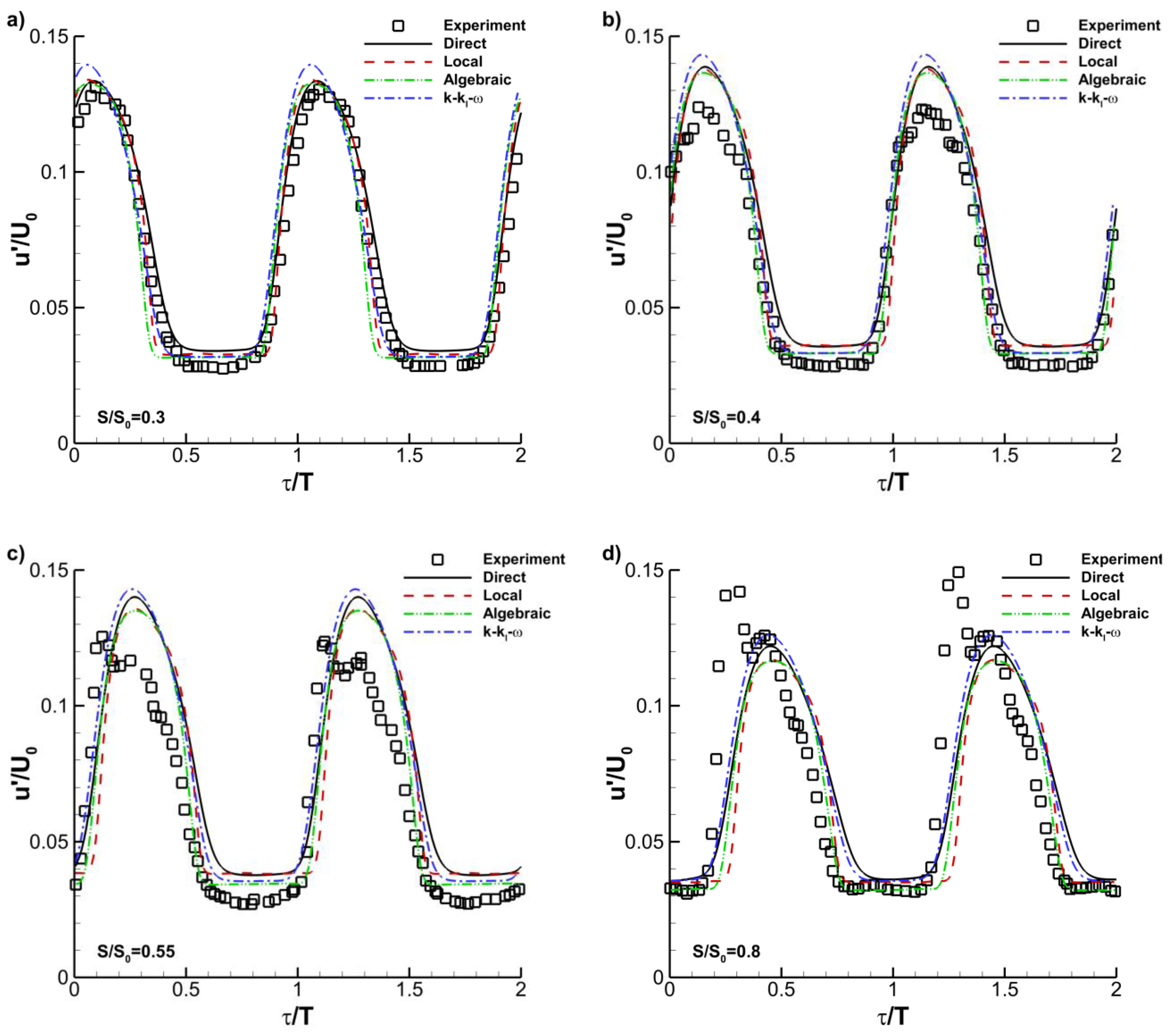
Figure 4 shows the comparison between computed and measured profiles of the fluctuating velocity component parallel to the blade surface,
u’ = (
2k/3)
1/2, at distance 10 mm from the suction surface of the blade at different locations for the wakes by 6 mm bars in a flow with background turbulence intensity
Tu = 3.0%. The fluctuating velocity is normalised by the mean velocity at the entrance to the cascade (
U0). The comparison is presented for two wake impact periods (
τ/T). The agreement between predictions and measurements is, overall, quite good. As said, this is crucial for a proper validation of the models. At the last location,
S/S0 = 0.8, a peak of
u’ is present in the experiment, which cannot be matched by the calculations. In the experiment, there is an increase of the free-stream turbulence towards the trailing edge, due to strong interaction between the moving wakes generated by the bars and the wakes of the blades [
147]. When a moving wake impacts on a blade wake, the blade wake is distorted and becomes very unsteady. The interaction causes large-scale eddies shed from the blade wake that break down into smaller fragments. The turbulence generated by this interaction causes an increased turbulence level in the free stream above the suction side in the trailing edge region. This interaction cannot be detected by a 2D URANS simulation.
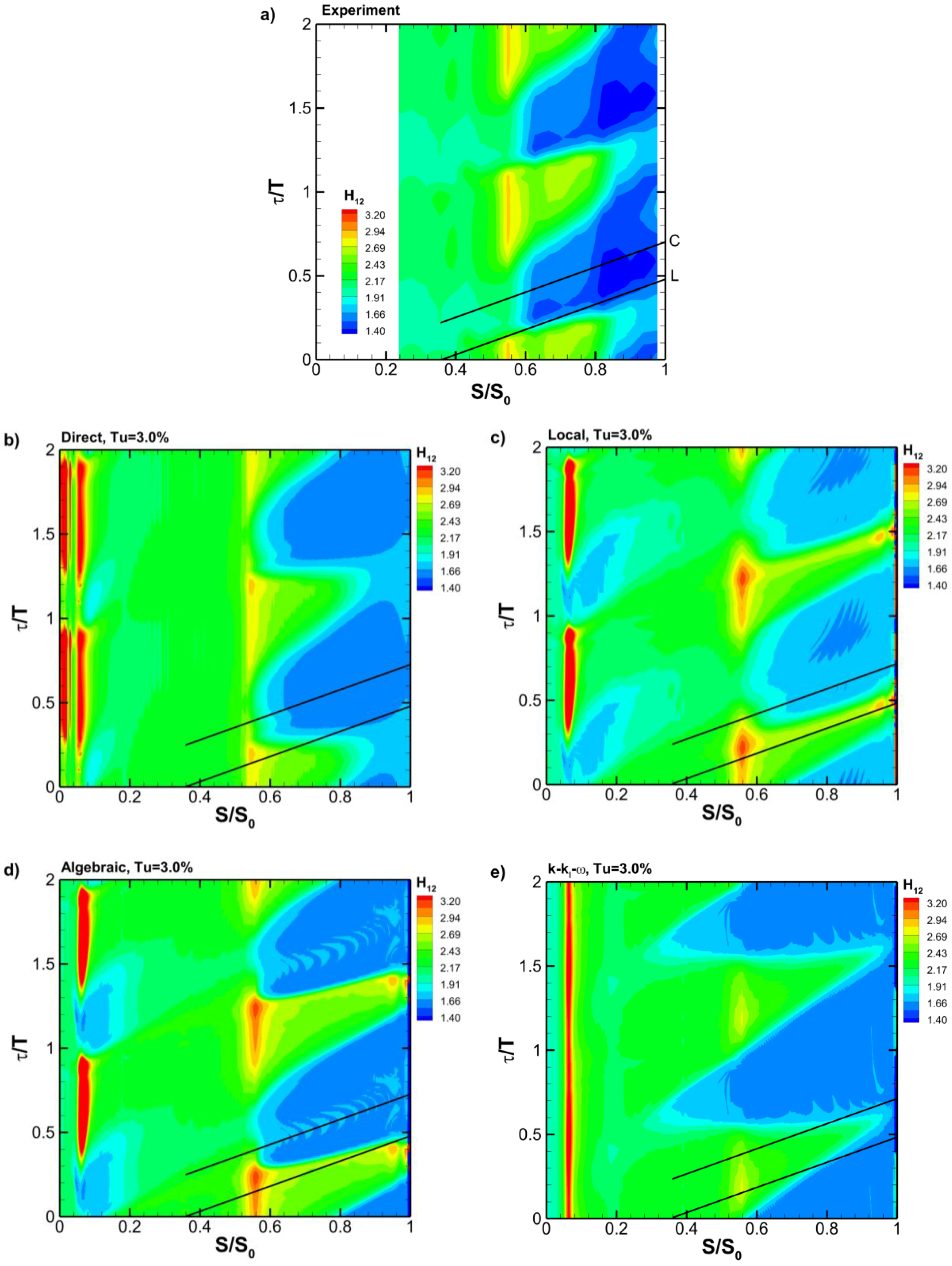
Figure 5 shows contour plots of the shape factor obtained in the experiment (
Figure 5a) and in the simulations (
Figure 5b–e). The two straight lines show the position of the moving wake. The bottom line (denoted L) corresponds to the leading edge of the wake and the upper one (denoted C) to its central part. The leading edge of the wake is the position at which local flow acceleration starts in the contour plots of the mean velocity (not shown) in the rear part of the blade (
S/S0 > 0.6). The central position of the moving wake is the position at which local flow deceleration starts. In the experiments, a fast transition to turbulence is observed under the wakes at
S/S0 = 0.6 and
τ/T = 0.2, caused by strong wake impact, as described in the section on mechanisms. The wake turbulence, which lags the front part of the wake (see
Figure 3), causes bypass transition. In the predictions, the best agreement with the experimental data is obtained by the direct intermittency model. The start of transition is somewhat delayed with respect to the experiment under the wake-impact (
S/S0 = 0.6 and
τ/T = 0.3), but the prediction agrees very well with the experiment after the wake passage. The local (
Figure 5c) and algebraic intermittency models (
Figure 5d) give good results in the turbulent zone, after the wake impact, but are more off in between wakes (
S/S0 = 0.8 and
τ/T = 1.0–1.3) near the trailing edge of the blade. The k-k
L-ω model (
Figure 5e) shows the largest deviations with respect to the experiment both under and in between wakes.
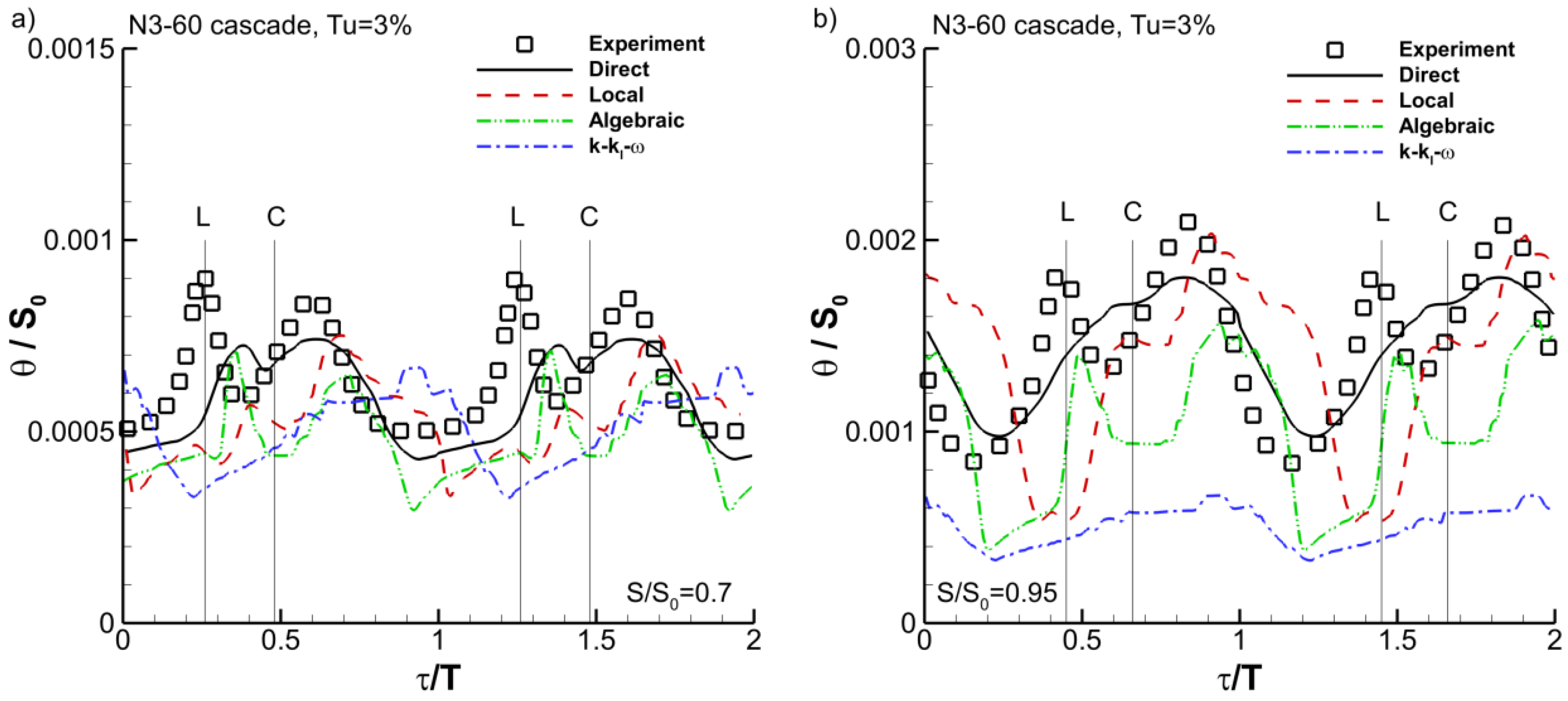
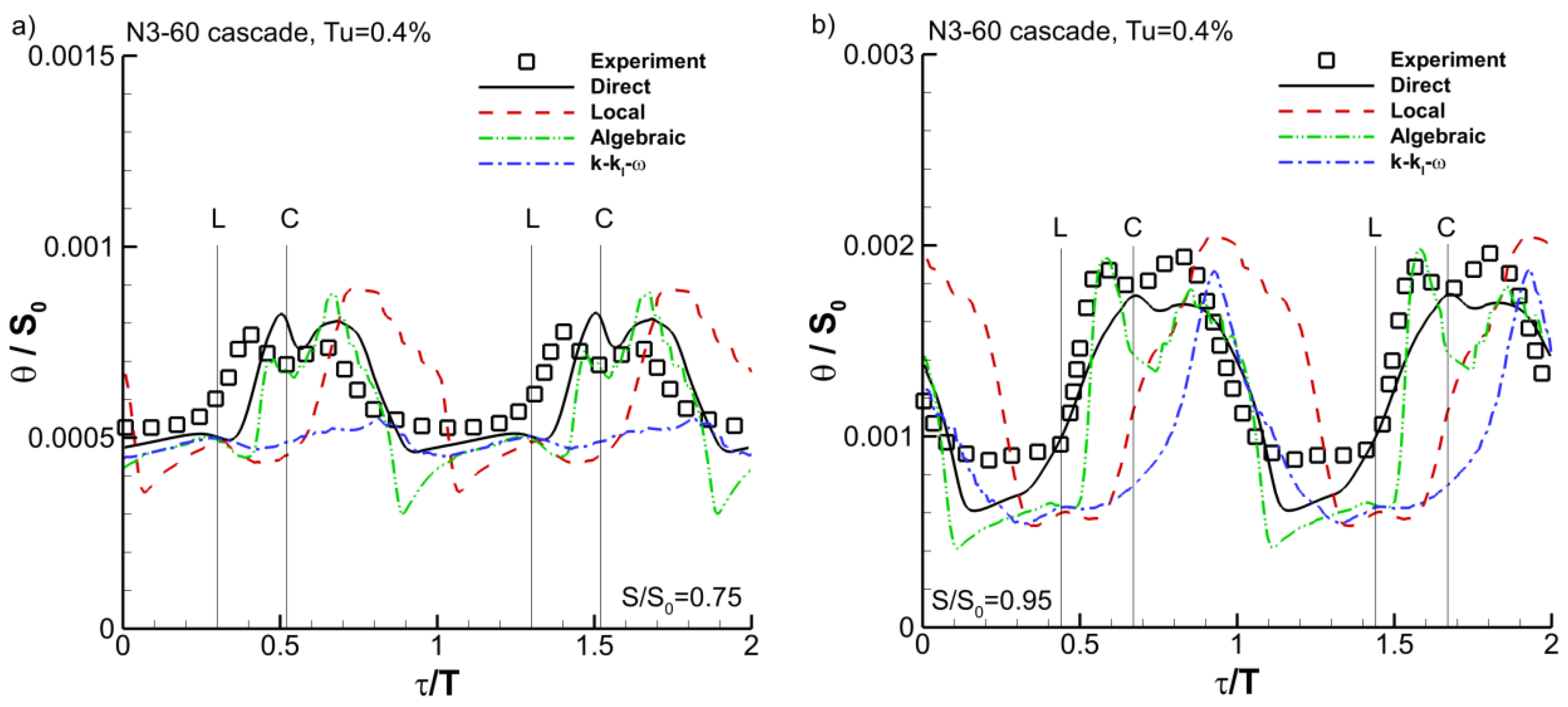
Figure 6 shows the evolution in time (two wake impact periods) of momentum thickness at two streamwise locations
S/S0 = 0.7 and 0.95. The momentum thickness is normalised by the length of suction side surface (
S0). The vertical lines are the positions of the leading edge (L) and central part (C) of the moving wakes. Two peaks of momentum thickness appear during one wake passage. The first peak is at the leading edge of the wake. The local thickening of the boundary layer is caused by the strong kinematic impact of the moving wake. This peak is too weakly reproduced by the intermittency models and missed by the k-k
L-ω model. Obviously, the interaction is stronger in reality than in the 2D-simulations, and, very likely, turbulence at the edge of the boundary layer in the simulations damps too much the interaction. The second peak occurs in the trailing part of the wake and is the result of turbulence created in the boundary layer due to bypass transition. None of the models produces the correct amplitude of the second peak at
S/S0 = 0.7 and 0.95, but the direct and local intermittency models are not far off. The mean value of the momentum thickness is well predicted at the tailing edge by the direct intermittency model, somewhat too low by the local intermittency model, more too low by the algebraic intermittency model and much too low by the k-k
L-ω model.
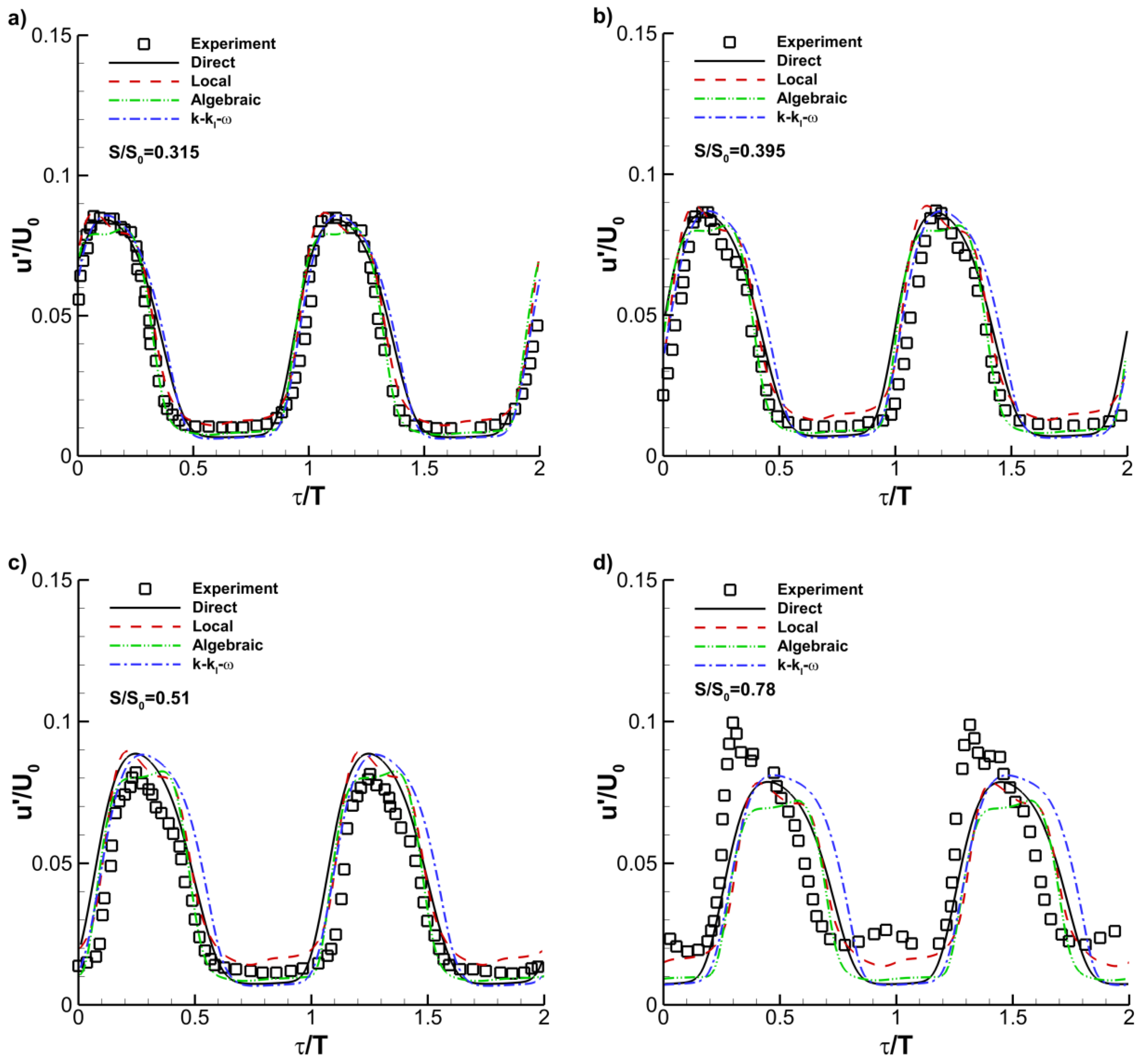
Figure 7 shows the comparison between computed and measured profiles of the fluctuating wall-parallel velocity component at distance 10 mm from the suction surface of the blade at
S/S0 = 0.315, 0.395, 0.51 and 0.78 for the wakes by 4 mm bars in a flow with background turbulence intensity
Tu = 0.4%. At the locations
S/S0 = 0.315, 0.395 and 0.51 the agreement between predictions and measurements is very good. At the last location,
S/S0 = 0.78, a peak of
u’ is present in the experiment, which cannot be matched by the calculations. Again, this peak is due to strong interaction between the moving wakes generated by the bars and the wakes of the blades [
147].
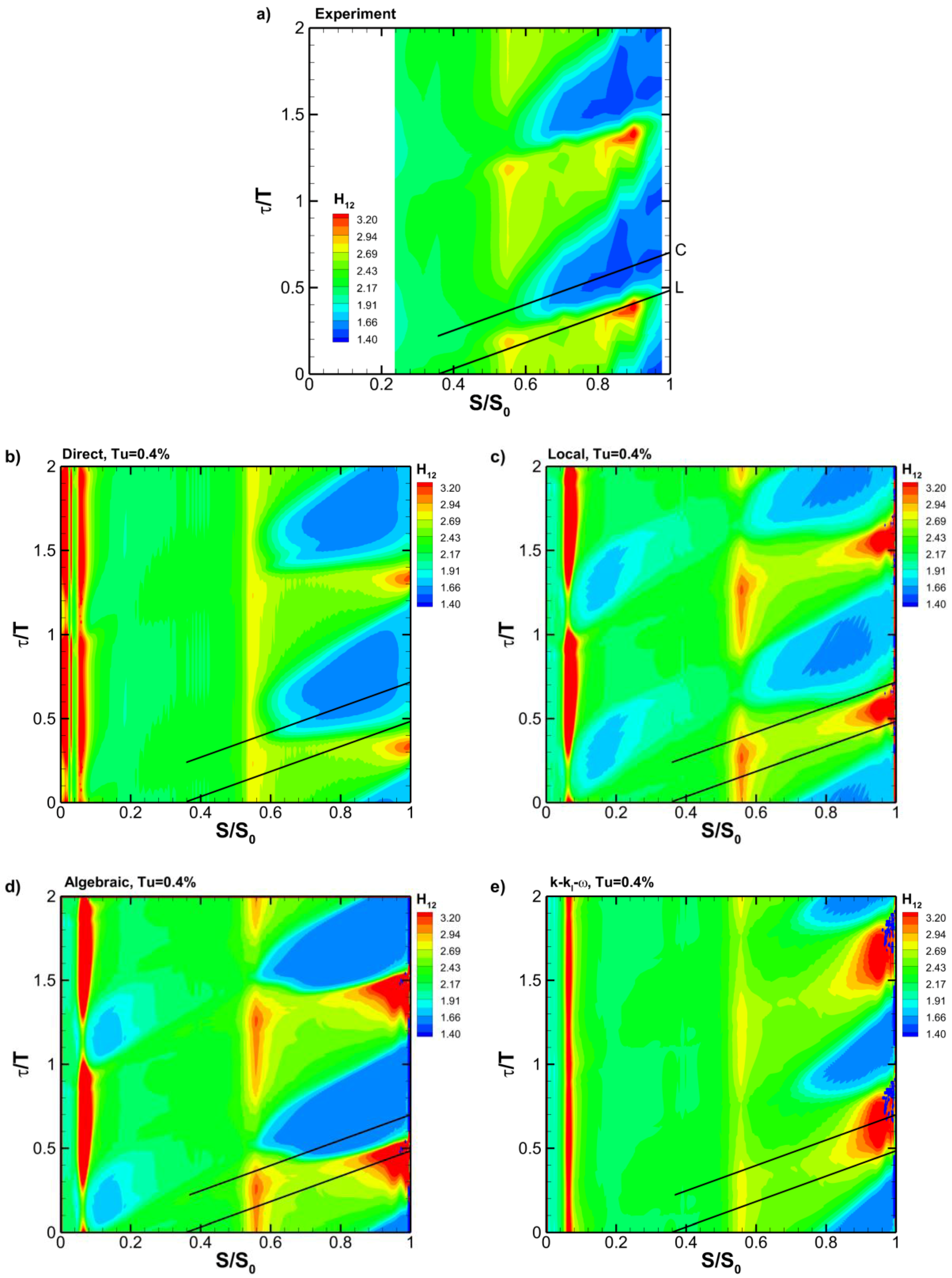
Figure 8 shows contour plots of shape factor obtained in the experiment (
Figure 8a) and in the simulations with the transition models (
Figure 8b–e). The direct (
Figure 8b) and the algebraic (
Figure 8d) intermittency models show good correspondence between prediction and experiment under the wakes (
S/S0 = 0.7 and
τ/T = 0.5). The transition to turbulence is underestimated somewhat in between wakes near to the trailing edge of the blade (
S/S0 = 0.9 and
τ/T = 0.1–0.4). Less accurate results are obtained with the local intermittency model (
Figure 8c) and k-k
L-ω models (
Figure 8e) both under and in between wakes.
Figure 9 shows the time-evolution of the momentum thickness at two streamwise distances
S/S0 = 0.75 and 0.95. The direct and algebraic intermittency models capture quite well the double-peak variation of the momentum thickness at both streamwise distances. The local intermittency model is able to reproduce the gross effect of the moving wake, but there is some delay in time. The k-k
L-ω model shows significant differences between simulation and experiment and the mean level is too low. The conclusion is that the mean value of the momentum thickness is well reproduced at the tailing edge by the intermittency models, but that the k-k
L-ω model produces a too low value.
Overall, the direct intermittency model performs the best. We consider this conclusion as quite normal for wake-induced transition dominated by the bypass mechanism. We are convinced that correlations are quite reliable for bypass transition such that a model by which the correlations are used in the most direct way is the most reliable. Further, the direct intermittency model has a specific model ingredient for strong wake impact, which helps much in improving predictions [
123]. Of course, a model using integral boundary layer quantities, which is thus non-local, has a drawback on computational efficiency. The results for the average value of the momentum thickness by the local intermittency model are quite good. But, there is a remarkable phase shift in the time-wise evolution of the momentum thickness with respect to the experiments and the flow is reproduced as too laminar in between wakes. The performance of the algebraic intermittency model is comparable to that of the local intermittency model. There is no phase shift in the time-dependent evolution of the momentum thickness, but momentum thickness is slightly underestimated and the flow is represented as too laminar in between wakes. The k-k
L-ω model underestimates the momentum thickness. We think that the deficiency may be partly caused by the use of a turbulence model that is very close to the standard k-ω turbulence model and that results may be better with a modern version of the k-ω turbulence model. When Walters and Leylek converted the first version of the model from a k-ε model [
87] to a k-ω model [
148], they introduced a supplementary diffusion term in the ω-equation (fourth term in the right hand side of Equation (56)) in order to improve the behaviour in the outer part of a boundary layer. It could have been better to start from a modern model with a cross-diffusion term in the ω-equation. We remark that the results reported by Walters and Leylek [
148] for wake-induced transition, but for cases with separation, were not fully successful.
The penalisation in computational efficiency of a non-local intermittency transport model with respect to a local one can be minimised by organisation of grid partitions in a parallel computation such that wall-normal lines for the calculation of the integral quantities do not cross grid partition borders, as demonstrated by Kožulović and Lapworth [
112]. Nevertheless, the calculation of integrals represents some overhead. In order to estimate this overhead, we recorded calculation times for 100 time steps in simulations on a single core of a 12-core computer of the flow across the N3-60 cascade. We compared the computing times for a k-ω turbulence model without transition model added, and with the added local intermittency γ-Re
θ transport model, our own non-local intermittency transport model and our own algebraic intermittency model. The SST k-ω turbulence model and the γ-Re
θ transition model are programmed within the ANSYS-Fluent package and, consequently, run inherently faster than the Wilcox k-ω turbulence model and our own transition models, which are programmed with the UDF functionality. We observed that the overhead due to the UDF can approximately be added by leaving it in an active state, even when it is not used. We set the convergence limits of the flow equations to the same value in all simulations and we take the computing time of simulations by the SST k-ω turbulence model with the UDF active and the Wilcox k-ω turbulence model (with UDF), which are equal, to 100%. The results are:
SST k-ω turbulence model with UDF active: 35.5 min = 100%;
Wilcox k-ω turbulence model (with UDF): 35.5 min = 100%;
SST k-ω turbulence model with UDF inactive: 33 min = 93.0%;
Local intermittency transport model with UDF active: 59 min = 166.0%;
Local intermittency transport model with UDF inactive: 50 min = 141.0%;
Non-local intermittency transport model: 63 min = 177.5%;
Algebraic intermittency model: 40 min = 112.5%;
Algebraic intermittency model + integral calculations artificially added: 42.5 min = 119.5%.
The supplementary computing time for the integral calculations is 119.5% − 112.5% = 7.0%. The local and non-local intermittency transport models both employ two dynamic equations for intermittency. The non-local one requires more computing time due to integral calculations and other non-local operations, such as distance determinations along path-lines. The computational cost of all these non-local operations is 177.5% − 166.0% = 11.5%. The supplementary computing time by the algebraic intermittency model is only 12.5%, which is much lower than the overhead of the local and non-local intermittency transport models, which are 66.0% and 77.5%.
14. Conclusions
We reviewed current models for modelling transition in turbomachinery boundary layer flows, with emphasis on the basic physical mechanisms of transition processes and the way these processes are expressed by model ingredients.
By the tests in the literature and our own tests it is not possible to come to a strong conclusion on the predictive qualities of current models. Successes by models are reported in the literature for some test cases, but failures are reported for other test cases. Also in our own test, we observe deficiencies. So, there does not seem to be yet a model that is universally successful. We remark that differences might be partly due to uncertainties on the free-stream turbulence level. The space-time evolution of the free-stream turbulence is rarely reported in measurements of wake-induced transition. This hinders model calibration and testing.
We think that the γ-Re
θ local correlation-based intermittency transport model by Menter, Langtry et al. [
75,
76,
77] functions overall quite well. This model has been used by many research groups and we are not aware of complete failures. However, there seems need for an improved model ingredient for transition in separated flow. We are also convinced that our own non-local correlation-based intermittency transport model functions quite well for turbomachinery applications. A useful ingredient in this model is the expression of strong wake impact, which makes results less influenced by the less reliable correlations for onset and growth in separated state. However, this model has the obvious drawback of being non-local. It is not possible to conclude on the new intermittency transport models by Menter et al. [
92] and Ge et al. [
94]. These are, very likely, not yet fully developed and not sufficiently tested. There can also not be a definite conclusion on our algebraic intermittency model [
88]. However, the last three models certainly have potential. So, it is probably a matter of further development and further testing. We are somewhat disappointed by the k-k
L-ω model of Walters and Cokljat [
85] for wake-induced transition. Successes of this model have been reported in the literature, but, as far as we know, only about tests with steady inflow. This model is not successful for our own test on wake-induced transition. We cannot judge fully on the qualities of the k-k
L-ω-I model of Pacciani et al. [
91]. This model is specifically designed for separated flow. Transition in attached boundary layer flow has to come from the transition by the low-Reynolds number functions in the turbulence model. We consider such an approach as not fully reliable.
Considering the ingredients of the current models, we can conclude that each model has at least one strong feature. Moreover, current models are not so much different than one would conclude from a first analysis of the models. Stressing the resemblances was one of the goals of our review. So, a positive last conclusion may be that ingredients from different models may be combined into models with better performance. We also believe that better understanding of the mechanics of transition in separated state, in particular, under wake impact, may help in further development of models. So, it seems to us that, although there is not yet a transition model that functions universally well for turbomachinery flows, such a model may not be very far away anymore.


