Determinants of Transport Mode Choice for Non-Commuting Trips: The Roles of Transport, Land Use and Socio-Demographic Characteristics


1
Department of Civil, Structural and Environmental Engineering, Trinity College Dublin, Dublin 2, Ireland
2
School of Architecture, Planning and Environmental Policy, University College Dublin, Belfield, Dublin 4, Ireland
*
Author to whom correspondence should be addressed.
Urban Sci. 2019, 3(3), 82; https://doi.org/10.3390/urbansci3030082
Submission received: 24 June 2019
/
Revised: 22 July 2019
/
Accepted: 23 July 2019
/
Published: 29 July 2019
Abstract
:Despite rapid changes in vehicle technology and the expansion of IT-based mobility solutions, travel habits must be changed to address the environmental and health implications of increasing car dependency. A significant amount of research focuses on commuting, which comprises the largest share of annual vehicle miles travelled. However, non-work trips are also significant, especially when considering trip frequency. Using empirical data (N = 1298) from an urban-rural region and bivariate statistical analysis, the relationship between the land use–transport configuration (6 types) and travel behaviour patterns is examined for 14 non-work destinations. The land use characterisation used in this research includes an updated means of representing a land use mix. By defining the typologies of land use and transport for use in the analysis, the findings can be directed towards contrasting area types in the region. A strong statistically significant association between the land use–transport configuration and mode-share for 14 non-work journey purposes is found. Using regression modelling, income and car ownership are identified as key influences on travel behaviour patterns. The results of both analyses show that, for non-work trips, the transport–land use relationship is as important as key socio-demographic indicators. However, the results for reductions in car travel are relatively small for the area typologies outside the inner-city core. This indicates that efforts to provide alternatives to car travel in order to mitigate car dependency should be prioritised in these outer urban areas. Appropriate management of spatial structure for non-work activity types such that active mode use is possible is essential. This will resolve some of the important environmental and health impacts of car dependency.
1. Introduction
At the city scale, it is expected that transport demand will double by 2050 within the Organisation for Economic Co-operation and Development area [1], with a corresponding doubling of car use, unless specific low carbon policy options are successfully implemented. Considering the scenario of maintaining the 2015 levels of private car use in cities, the International Transport Forum [1] suggests that 70% of emissions reductions could potentially come from new technologies, but that 30% need to come from changes in human travel behaviour. There are important health consequences, especially for children, of encouraging higher shares of active transport mode use [1,2,3].
The extent to which the urban form influences people’s travel patterns has long concerned researchers and policy makers. Efforts to promote the use of sustainable travel modes (walking, cycling, and public transport) have been less effective than expected, with some researchers concluding that many regions can now be classified as ‘car dependent’ [4,5]. To reduce car dependency, alternatives to car travel are required. The availability of these alternatives and its effect on the mode-share for non-commuting trips is the subject of this paper. Empirical data from a medium sized European city-region are used to explore the determinants of the mode-share and the level of car dependency in different areas within the region.
Despite a considerable research effort in understanding car dependency, policy responses to reduce it have been limited. While it is clear that higher densities support less car use, it is less clear how to provide for alternatives to car use in areas with very dispersed development patterns. The lack of emphasis on non-commuting trips may have contributed to this, as well as the difficulty of understanding which parts of the urban form influence which elements of travel behaviour [6]. The research presented here addresses this imbalance by examining the effects of contrasting urban forms (i.e., not all compact development) on travel behaviour. The development of a bespoke means of characterising land use–transport typologies is an approach adapted specifically to non-work trips, which is relatively less well covered in the research literature. A key component is the land use mix, as this affects, in large part, the distances to be travelled for non-work activities. A novel means of formulating the land use context for non-work trips is presented as part of the analysis here.
1.1. State of the Art
Litman describes car dependency as a “self-reinforcing cycle of increased car ownership, reduced travel options and more dispersed car-oriented land use patterns” [5]. This concept underpins the analysis, presented here, on non-work trips, in that car ownership, travel options and land use patterns are the principal elements. It is well-established that the urban form has an influence on travel behaviour, but by way of analysis and measurements, there are multiple methodological and theoretical stumbling blocks [6]. In fact, the direction of the relationship and a conclusive result as to which parts of the urban form influence which elements of travel behaviour remain elusive [7,8,9]. Knaap et al. [9] suggest inter alia that the effects of increasing density will depend, to a significant extent, on the existing density within a specific space or population. This means that efforts to increase density, as a planning response, may not have the intended outcome. Meanwhile, Handy [8] points to methodological issues in addressing this relationship and claims that much of the available research is framed too narrowly. Moreover, she suggests that additional measures are required to reduce car use, apart from compact development.
Stevens [10] revisits the question in a recent study, using a meta-analysis and regression analysis to evaluate the literature from the period 1996–2015, and examines whether compact development results in a reduction in vehicle miles travelled (VMT) and, if so, what the magnitude of this effect is. He finds that, while overall, there is a reduction, the effect may be smaller than that generally understood or expected by planning practitioners. His results show that the strongest influence on VMT is the distance to downtown or the city centre, with an elasticity of −0.63. This shows that, if the distance decreases by 1%, a household’s driving goes down by 0.63% on average. He also presents the household or population density, with an elasticity of −0.22, which shows that people drive less in areas with higher densities. However, he also recognises that increasing the density in a city is a very difficult process. He shows that, if a city is successful in increasing the density by 40%, driving trips might decrease by 9%.
To investigate, in detail, the potential for land use–transport system interactions in order to increase the use of sustainable transport modes (walking, cycling and public transport), the analysis described in this paper develops an accessibility measure (composite measure), as well as land use measures, e.g., the residential density (direct measure), proximity and intensity of retail facilities (land use mix measure) and socio-demographic factors.
This expands on the axiom presented by Ewing and Cervero [7], which states that individual trip generation is primarily influenced by socio-demographic characteristics, and trip distances mainly influenced by land use patterns and socio-demographics constitute a secondary factor. Increasingly, a range of other factors, such as life stage, life style, psycho-social and attitudinal factors have been shown to influence non-work travel behaviour patterns [10,11,12,13,14,15,16,17].
1.2. Operationalising the Research
Litman [18,19] summarises the wide range of meanings and considerations afforded by the term accessibility with an emphasis on how different practitioners understand it (e.g., transport planners—mobility and traffic; land use planners—distance, time and communications; and connectivity and social service planners—ability of those with additional needs to access services). Meanwhile, Geurs and van Wee [20,21] provide a detailed account of both the theoretical underpinnings and the minimum expectations of the term, as applied in the evaluation of integrated transport-land-use planning. They note that the complexity involved in incorporating four distinct elements, comprising land use, transport, temporal and individual components, means that, in practice, researchers and practitioners tend to rely on a particular perspective to suit their needs (see [20] for a full treatment of this).
As a minimum for transport planning and land use planning, accessibility is defined as the distance to a particular activity (see, e.g., reference, [22]), while in studies of non-work trip destinations, it is often adapted for specific activities. For example, Fan and Khattak [23] define four indicators of accessibility, specifically for retail and dining. These include both count and distance measures. Prior to the development of accessibility, as a means of both analysing and evaluating land use–transport strategies in the evolution of approaches to transport planning (see, e.g., reference [24]), much of the literature relies on the five Ds, despite the known limitations (see, e.g., references [25,26]). As Stevens [10] sets out, the five Ds typically refer to:
- Density: Population, households or jobs per unit area
- Diversity: Mixture of different land uses, often represented by the land use mix variable, and sometimes the jobs-housing balance
- Design: Street network characteristics: the density of intersections and proportion of intersections
- Destination accessibility: How easy it is to access trip destination: the distance (often to the city centre)
- Distance to transit: Distance from a household to the nearest stop
In the current analysis, a composite accessibility measure is computed, which includes both the proximity to public transport, as well as the level of service variable. Meanwhile, density is included as a residential density factor (dwellings per hectare), and diversity is incorporated by way of the land use mix.
Land use mix factors are discussed in the literature by Boarnet and Sarmiento [27], who highlight that the variation in approaches to examining non-work travel behaviour patterns is due to the plethora of indicators and conceptualisations used to operationalise research. The land use mix is especially important in relation to non-work trips, as it has a large bearing on distances to reach different types of activities. Gehrke and Clifton [28] describe the conceptualisation of the land use mix as including three elements: land-use interaction; geographic scale and temporal availability. In considering the land use mix, they propose the classification scheme of Song and Rodriquez [29] and Brownson et al. [30], as set out below:
- Accessibility (distance based): Not always considered a land use mix measure
- Intensity of the activity type: A count or percentage—the number of opportunities related to a land-use type within an area and/or the percentage of land in a defined area dedicated to the activity
- Pattern: Spatial pattern identified as the variety of land use types within an area (composition) and their proximity to one another (configuration)
Here, we rely on a composite indicator—accessibility—which includes both spatial and temporal elements. The temporal aspect relates to the frequency of the public transport service (referred to as a level-of-service in the transport planning literature (see, e.g., reference [18])), rather than the availability of land uses (as suggested by Gehrke and Clifton [28]). It is a composite measure, as it also includes the distance to the bus stop or rail station. This is important, as accessibility has historically been considered from the perspective of planning for cars, rather than public transport modes and active modes (walking and cycling). Elements of the pattern (as defined above) are encapsulated using another composite measure. The intensity of retail activities, combined with sufficient proximity to residences to provide for active transport is computed (regardless of the availability of public transport infrastructure or walking and cycling infrastructure). This approach follows Rajamani et al. [31] but diverges from Boarnet and Sarmiento [32], who use retail and service employment density. While individual measures of each land use variable have been used in other regression analyses, a system of six land use transport typologies (LUTTs) was developed for use in the current study.
1.3. Selecting Indicators for Non-Work Travel
Environmental concerns linked to the share of carbon emissions from the transport sector in contributing to climate change has caused policy efforts to focus substantially on the area of CO2 emissions reductions [33,34]. Vehicle kilometres travelled (VKT) is a key indicator and reducing VKT leads to reductions in emissions. There is a strong health imperative associated with increasing active transport in combatting increasingly sedentary lifestyles [2,3], and it appears that there is an untapped potential with respect to non-work journey purposes. In addition, while replacing fuel types for car travel reduces emissions, the health benefits of active transport are not accrued. Therefore, it is important to consider the mode-share and encourage active transport use (and public transport use), as a means of improving health outcomes as well as the condition of the environment [2,33].
Non-work trips have both a higher frequency and comprise a higher proportion of trips than commuting trips (e.g., data from England suggest that non-work journeys accounted for over 85% of all trips in 2017 [35]). In addition, there are socio-demographic segments that are not formally working (commuting), and their travel behaviour and options for sustainable transport use are overlooked in traditional analyses of commuting travel behaviour.
Commuting trips tend to be longer than non-commuting trips (for example, in England, the average distance travelled for commuting trips was 1309 miles per person per year in 2018, whereas for retail, it was 738 miles per person per year [36]). However, in the under-researched area of non-commuting travel, alternative indicators to total vehicle kilometres, such as trip frequency (trip rate) and mode-share by journey purpose, are also important [31,37,38,39]. This is, in some part, due to the heterogeneity of the spatial structure for non-work activities. Handy notes that opportunities available to residents must be evaluated in some detail to capture subtle differences in the urban form. Additionally, the quality of an available choice must be evaluated in terms of its availability [37]. For example, being close to a high-speed railway service, a high-quality service, is irrelevant, if the frequency is low, or it does not stop at the local station. In that case, its availability is poor, or its quality is low. There are also considerable limitations regarding the provision of public transport in low-residential-density areas, which considerably reduces the available options (e.g., reference [37]).
Chatman [38] uses non-work travel frequency as a key indicator (dependent variable), while distance measures are included as independent variables. Rajamani et al. [31] describe non-work travel behaviour using the mode-share per trip type, rather than distance. Handy [37] relies mostly on the destination choice, variety of destinations, factors influencing the choice, mode choice and trip frequency, rather than the average distance, in her analysis. Boarnet and Sarmiento [32] rely on the frequency of non-work trips, as the key dependent variable in their analysis.
In the analysis in this paper, typologies of land use transport characteristics are defined using a spatially explicit method. Six categories (land-use-transport types [LUTTs]) are used to compare the travel behaviour of residents in different area types. In this way, the level of possible active transport use is implicit in the categorisation of the LUTT. This is important, given the variations in the spatial pattern of the road and transport network across the region and the differences in accessibility by walking and cycling, compared with car use. Previous studies are usually drawn from areas with grid-like street patterns, where it is normal to use the number of road intersections as a measure of connectivity (see, e.g., references [27,40]). However, given the heterogenous road pattern in the study region, this measure has been omitted from the current analysis. In addition, the interpretation of the results is more readily targeted at specific land use transport types and provides for a more robust specification of the policy requirements. The method for defining the typologies is presented in the Materials and Methods section.
1.4. Socio-Demographic Effects
The influence of socio-demographic effects on travel behaviour is well-established. Researchers often rely on car ownership levels, as a key indicator influencing travel behaviour patterns, as undoubtedly households with higher levels of car ownership tend towards higher shares of car use. However, as noted, this type of analysis does not necessarily elucidate whether there are viable alternative options in place (for example, distances to facilities that are suitable for walking and cycling and high-quality public transport). In a case in which there are available alternatives, it can be argued that subjective factors may influence the persistence of high levels of car use. Clearly, if there are no alternatives, it is more challenging to provide viable policy solutions to reduce car use. It is in those areas, where there are alternatives, but car use is still high, that there is opportunity to look at policies to encourage alternative behaviours [41,42,43].
Stead [14] argues that socio-economic factors have a greater influence on travel patterns than do land use factors. Meanwhile, Buehler [44] compares the use of active and public transport modes in the USA and Germany. The presence of a car, while facilitating car-based transport, does not necessarily lead to car use, as developed in Buehler’s study [44]. He compares the levels of car use in the US and Germany and highlights the effects of the availability of alternatives. While both have high levels of car ownership, in Germany, the shares of active and public transport trips are four times higher than those seen in the US. This is because, in Germany, active transport use is supported by the spatial structure and appropriate infrastructure. In contrast, Susilo et al. [45] found, in a UK study, that even where supports are in place for active transport, both for commuting and non-work trips, there remained a preponderance of car use.
To explore both the influence of land use–transport characteristics and socio-demographic factors on non-work travel behaviour, the study addresses the following key research question by proposing four sub hypotheses. In this way, an understanding of the level of car dependency in different area types can be investigated and expand on the overall research question: What factors influence the mode-share for non-work trips?
- Do contrasting LUTT characteristics have a similar effect on different types of non-work trips?
- What is the difference in magnitude between the effects of each LUTT on the proportion of trips by a sustainable transport mode (aggregated for all 14 destinations)?
- How important are income and car ownership in determining the mode-share for non-work trips?
- How is income related to the level of car ownership and volume of non-work trips?
2. Materials and Methods
2.1. Geographical Setting
The study region, The Greater Dublin Region, comprises the administrative areas of the 4 local Dublin authorities and the surrounding counties of Louth, Meath, Kildare and Wicklow. The region accounts for the majority of the population and jobs in the country, with 834,033 recorded as over the age of 5 travelling to work, school or college in the 2011 Census [46]. The total population was 2.034 million in 2016 [47]. It comprises a range of settlement types and provides urban, suburban, peri-urban contexts, as well as rural towns and villages, and therefore offers a suitable study region to examine land use–transport interactions. Six mutually exclusive land use–transport typologies are defined in the region using spatial analysis techniques.
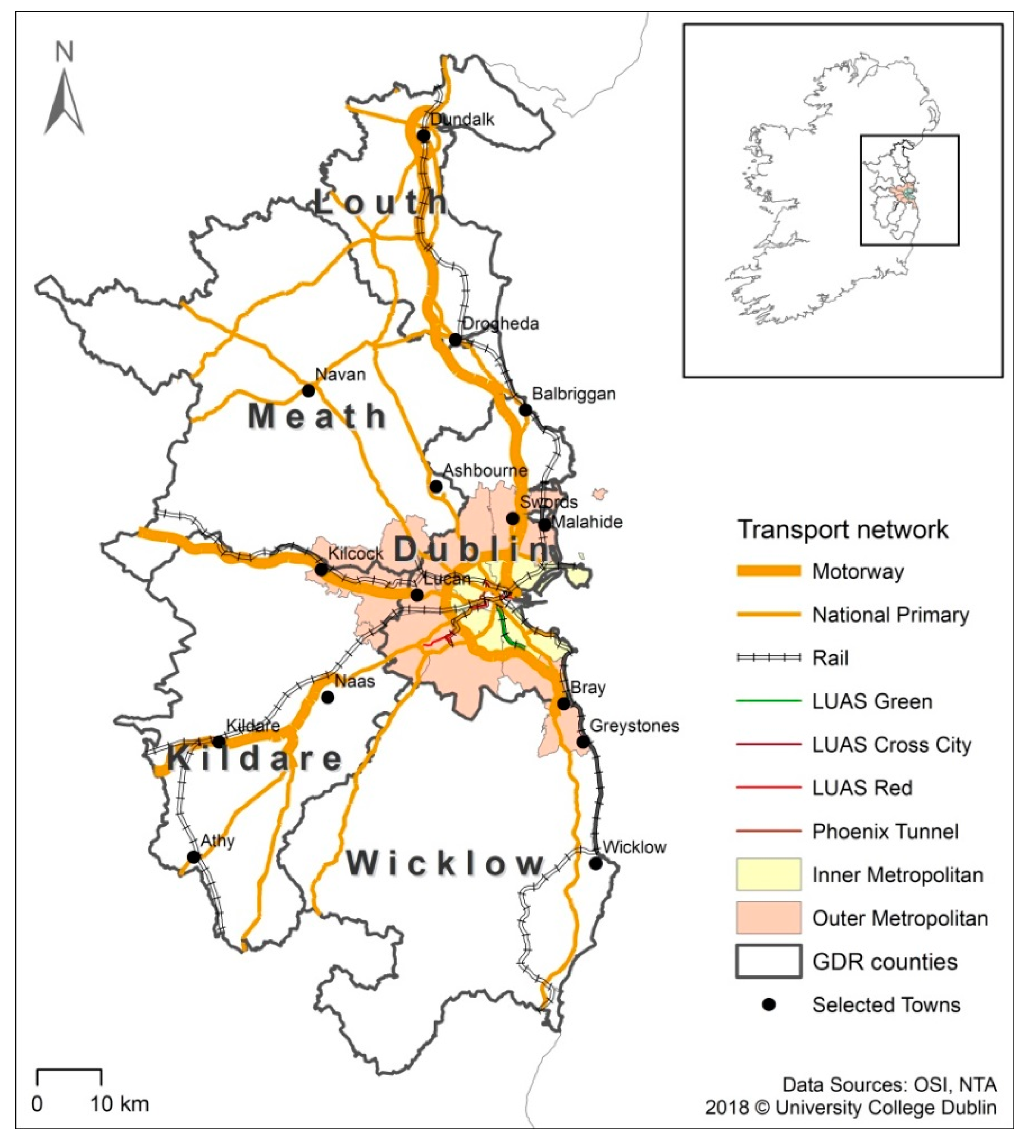
Figure 1 shows the study region (which comprises the counties of the Greater Dublin Area (GDA), as well as County Louth), which borders with Northern Ireland to the north. Major transport infrastructure in the region is shown to include the motorway and national primary road system, the inter-city rail system and the tram system (LUAS). The development of transport infrastructure over time has impacted on the spatial development patterns in the region, as experienced in cities around the world [39,48]. The areas defined by the National Transport Authority [49] are also shown in considering strategic plans for the region. They include the Outer Hinterland areas, the Inner and Outer Metropolitan areas, as well as the inner-city core, which can be seen in the map inset. As shown in [50], the region illustrates a sprawl type of development pattern, similar to that seen in other European regions, for example, Flanders, Belgium and the Cardiff region, Wales [50].
The residential density in the study region ranges from very low, for instance, in the mountainous areas in Wicklow (0.01 dwellings per hectare (dpha), to the highest, which is found in the Docklands area of the city centre (555.1 dpha). Graby and Meghen [51] show that, in the Irish context, the average dpha in urban areas is 258 dpha; in inner suburban areas, it is 96 dpha; in outer suburban areas, it is 66 dpha; and in towns and villages, it is 80 dpha. This is used as the basis for the categorisation used in the definition of LUTT (see the section, entitled ‘Definition of Land Use–Transport Types’). It is acknowledged that these figures represent the Irish context, which, in international terms, is low-density. For example, Robinson [52] describes high-density in the Netherlands as in the region of 300 dpha in the high-density central docklands of Amsterdam. Van & Senior [53] provide indicative residential densities for Cardiff, Wales of 19.2 dpha, in the inner urban area of Canton, which comprises the inter-war terraced and semi-detached properties, and 28.4 dpha in Fairwater, which is mostly residential, containing a mix of high-rise flats and private and local authority housing. However, recent guidelines suggest that higher densities of 30–45+ (net dwellings per hectare) are required for new developments [54].
2.2. Data
Primary data on non-work travel behaviour were gathered by means of a self-completion household survey. The objectives of the survey were to examine, in some detail, the mode choice for a range of journey types and to gather data on other factors that may be linked with mode choice selection for these journeys, both land use elements and other socio-demographic, behavioural and attitudinal characteristics. A total of 272 variables were defined in the survey. Questions relating to attitudes to transport modes were adapted from previous research by Van Acker [17]. This included collecting data on peoples’ orientation to different transport modes and their perceptions regarding the attitudes of family and friends towards their transport mode choices.
The sampling strategy was designed to ensure a sampling fraction of at least 1% of households in each of the land use transport typologies. In addition, the minimum requirement for the robustness of the results was applied, as per Cochrane’s Sample Size for a Known Population (cited in reference [55]), using a confidence level of 3%, which is below the widely used 5% minimum [56,57] (See Appendix A for details of the calculation). The calculation gave a minimum sample size of 798.
Descriptive statistics were run using SPSS v20 software to indicate the frequency and range of responses. An effective sample of 1298 respondents was achieved, following the processing and cleaning of the data. This represents a 21% response rate (see Table A1, Appendix A).
A range of secondary datasets were used in both the definition of the land use transport types and in testing the representativeness of the sample, prior to the completion of the analysis. These include the 2011 Census [58], Small Area boundaries [58], location of transport stops and stations (dublinked.ie), General Transit Feed Specification from transport agencies, timetable information (irishrail.ie, DublinBus.ie, hittheroad.ie), statutory planning documents and An Post Geodirectory (version 2013). This is an address database of all address points in the country, grouped by economic activity category. The categorisation follows a pan-European system called NACE. The Geodirectory database provides a NACE Code, NACE Code ID and Category in the NACE_CODES table.
2.3. Definition of Land Use–Transport Types (LUTTs)
Standard spatial analysis tools were used to identify mutually exclusive sets of small areas. (Small areas are areas of the population comprising between 50 and 200 dwellings, they are nested inside electoral divisions). The selection was made based on criteria comprising both spatial and temporal aspects.
The residential density (dpha), proximity to public transport stops (bus, rail, light rail, and tram) and distance to a retail cluster (see reference [59]) were calculated. The residential density was categorised into three bands, 0–55 dpha; 55–240 dpha and >240 dpha. In general terms, a density higher than 240 dpha was evident, close to public transport nodes, in areas with apartment block-type developments, which have been encouraged at the policy level, while in rural areas, the general density was below 55 dpha, which reflects dispersed settlement patterns, germane to rural Irish areas. Public transport stops were coded based on the frequency of service in a reference hour to reflect off-peak service availability (3–4 pm on a weekday to ensure that schedules arising for the after-school period and before the peak commuting period were not included in the reference hour to represent the off-peak service frequency). The proximity to the stops was also included, and small areas were selected as having access to the specified level of service frequency, when within a 1 km range of LUAS and train stops and within a 500 m range of bus stops. This reflects people’s willingness to travel further to a higher-frequency public transport service, although research indicates that context is important [60]. The approach taken in this research could be replicated in other study regions, depending on the availability of similar spatial datasets.
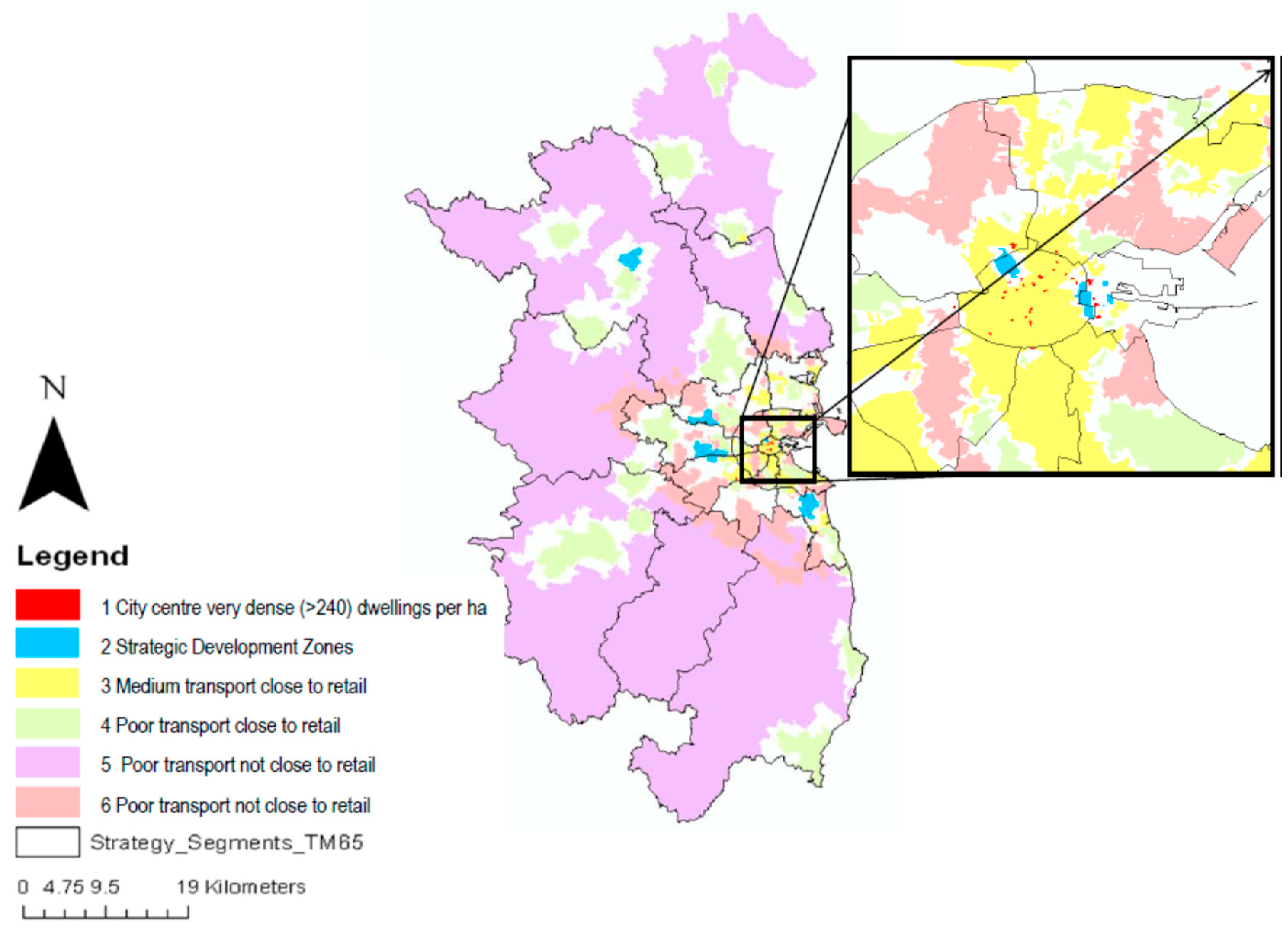
The spatial extent of the six LUTT typologies are displayed in Figure 2. LUTT2 is different from the other LUTTs in that these areas were selected due to their designation as Strategic Development Zones (SDZs). The designation is a statutory, special planning framework which was introduced in 2000 to serve as a fast-track process for delivering development of economic or social importance to the State [61]. While the designation can apply to industrial, residential and commercial development, the interest in this case is in the delivery of sustainable neighbourhoods. A key aspiration in these zones is to ensure the phased development of infrastructure in tandem with or before residential occupation.) within the State planning system. A summary of the characteristics of each LUTT is presented in Table 1. The socio-demographic characteristic of each LUTT is shown in Table 2. The average household size ranges from 2.03 in LUTT1 to 2.96 in LUTT5. This shows that LUTT1 has a more compact urban form (taller buildings and apartment blocks), whereas LUTT5 contains larger family homes, built in a dispersed pattern (one-off housing), where a lower pressure on land values results in larger homes (on average). There are significantly fewer Small Areas with higher density dwellings (LUTT1 = 40, LUTT2 = 108), compared with LUTTs 3–6.
2.4. Sampling and Tools
A two-stage random probability stratified sampling strategy was adopted for the study. The overall population of households in the region was stratified based on the six defined typologies (see description in the next section). Postal addresses were then selected at random from each stratum using the An Post Geodirectory database and the random number generator in MS Excel.
Standard spatial analytic functions in ESRI ArcGIS 10.1, such as select by location, were used to ensure that the small areas in each typology were only present in one typology. Buffers, standard SQL queries and some additional tools (e.g., the ‘Display GTFS Route Shapes Toolbox’ (https://esri.github.io/public-transit-tools/DisplayGTFSinArcGIS.html.)) were used to codify the stops (train and bus) with both the frequency of service and proximity.
2.5. Statistical Tools
Standard bivariate and multivariate techniques were used in the analysis. Chi-square tests were applied to examine the relationship between the observed and expected frequencies of the mode selection. The Chi-square test determines if there is a statistically significant association in the data, and measuring the effect size gives an indication of the strength of the effect between the variables. Cohen’s criteria [62] are used in the analysis, as shown in Table 3. Even a small effect can be statistically significant, if it is observed in a very large sample [57]. Two measures are used in the analysis. To measure the effect size (r2) for a 2 × 2 matrix, the phi coefficient is used, whereas for a larger matrix, Cramér’s V is used.
A One-Way Anova test was used to determine if there is a statistically significant difference between the means of two or more independent groups [63]. For example, the proportion of all non-work trips that are carried out using sustainable transport modes, compared with all modes, is measured for each respondent. The measure is a proportion, expressed as a fraction, and has a value between 0 and 1 to show the proportion of the trips that are carried out by sustainable transport modes. The mean value of this variable is computed for each group of respondents, and they are grouped based on the LUTT at the residence. A key requirement of the One-Way Anova is that there is homogeneity of variances. In the example, in the analysis, the test (Levene’s Test) of the Homogeneity of Variance was violated (as it was significant, p = 0.001), and Welch’s ANOVA was therefore reported instead, as it is not sensitive to this issue [63]. The one-way ANOVA is an omnibus test statistic and therefore cannot determine which specific groups were significantly different from the others. In this case, a post-hoc test was used to provide this information.
Correlation analysis is used to describe the strength and direction of the linear relationship between income and car ownership. The Spearman Rank Order Correlation (rho) is designed for use with the ordinal level or ranked data and can be used, if the requirements for the Pearson product-moment correlation coefficient are not appropriate [64].
2.6. Regression Modelling
Multivariate techniques make it possible to undertake deeper analyses that can consider causal mechanisms, beyond mere association or correlation [65]. Regression modelling consists of a family of techniques that explore the relationship between multiple independent variables and a dependent variable.
3. Results
In this section the key research question looking at what factors influence the mode-share for non-work trips is addressed through the analysis associated with each of the four sub hypotheses. The results show that, in areas where compact development objectives, with supporting high-frequency public transport, can be met, there is an associated reduction in car use (LUTT1). However, in areas with lower residential densities and differing levels of public transport availability, there are significant challenges to reducing car dependency (LUTT2–LUTT6). More importantly, despite significant differences in public transport frequency between LUTT3 and LUTTs 4–6, the mean level of the proportion of total trips by sustainable transport modes was not of a comparable magnitude. Using both the measure of accessibility and the novel land use interaction measure related to retail intensity provided a new means of characterising the land use–transport characteristic of each area. While this approach was used in response to the research needs in the literature, the findings, presented here, did not diverge significantly from those presented in the existing literature. Thus, the results add to the body of evidence indicating that land use transport interactions must be considered in finding solutions to car dependency. The supply of bespoke communal transport options and more effective ways of managing land use patterns in these areas are essential.
Given that the journey purposes with the highest levels of car use were retail, family and friends, sports centre and swimming pool visits, these activity types should be prioritised in focusing efforts to provide alternatives to car use. The results show that, where distances allow for walking or cycling, respondents can reduce their car use. The location of local medical centres/doctor’s surgeries, pharmacies, post offices and local shops is shown to be effective in supporting active transport use, despite lower residential densities and dispersed settlement patterns. Activity destinations for sports, swimming, visiting friends and family and retail feature higher levels of car use. This is often due to retail clustering at the edge of town developments, chosen primarily for their high accessibility by car, but with active and public transport facilities often overlooked. The highest levels of public transport use were seen for trips to the cinema, theatre, social club and classes. This demonstrates that the clustering of these activity types can support sufficient patronage levels for public transport services. However, it may also be due to the co-location of work places and mixed-use activity centres. The next sections set out, in detail, the results of the analysis, carried out to address the research sub-hypotheses.
1. Do contrasting LUTT characteristics have a similar effect on different types of non-work trips?
As shown in Table 4, for each of the 14 destinations included in the survey, the proportion of people who use a car to reach them, compared with those who do not, was statistically significant (p < 0.001). The strength of the association is assessed using Cramér’s V values, which are shown in the column on the far right. The strongest association was for the cinema and INTREO (social welfare office) trips (Cramér’s V > 0.4), followed by the theatre, swimming pool, sporting centre and class (Cramér’s V between 0.39 and 0.338), with the weakest association for the pharmacy, post office (PO), General Practitioner (GP), local shop, supermarket shop, family and friends and worship (Cramér’s V between 0.319–0.21). The results show that whether someone chooses to use a car or other modes of transport is associated with the LUTT characteristics of their place of residence. There is some variation between the destination types and the strength of the influence of the relationship between the land use–transport characteristics and mode-share for each trip type. LUTT1 shows consistently higher shares of non-car use for almost all journey purposes, compared to LUTT4, LUTT5 and LUTT6. Considering each destination type in detail, Table 5 shows the destinations with the highest shares of each of the three main modes: Active mode, car, and public transport.
2. What is the difference in magnitude between the effects of each LUTT on the proportion of trips by a sustainable transport mode (aggregated for all 14 destinations)?
To investigate the mode-share for non-work journey purposes, an analysis was conducted to compare the effect of each LUTT on the proportion of sustainable transport mode use (active and PT). The results show that the mean proportion of trips by sustainable transport modes was statistically significantly different between each LUTT, Welch’s F (5, 164.2) = 15.5, p < 0.005 (see Appendix B). This means that the proportion of trips carried out by sustainable transport modes, compared with all trips by all modes, was statistically significantly associated with the land use–transport typology of the respondent. It was statistically significant in the case of residents of LUTT 1, compared with each of the other LUTTs at a high level of significance, and it was statistically significant in the case of residents of LUTT3, compared with LUTT4, LUTT3 with LUTT5 and LUTT3 with LUTT6, at a lower level of significance. The mean for each LUTT is shown in Table 6, with the standard deviations. A Games-Howell post-hoc analysis revealed that the difference between LUTT1 and LUTT2–6 was statistically significant. In addition, the differences between LUTT3 and LUTT4, LUTT3 and LUTT5, and LUTT3 and LUTT6 were statistically significant, as shown by the confidence intervals and p values presented in Table 7.
LUTT1 demonstrates the highest levels of active and public transport use, aggregated for all non-work journey purposes. The levels seen in LUTT1 are almost twice that in any of the other LUTTs. Additionally, the magnitude of the difference in active and public transport shares is small between the other LUTTs and in comparison with LUTT1. This proves that a higher-density mixed use development, with high-quality public transport, supports the use of the sustainable transport mode. Moreover, it shows that the difference between having medium-level transport services, compared with poor transport, and being distant from retail clusters (as in the case of LUTT5 and LUTT6), has a strong negative influence on the level of the use of the sustainable transport mode for non-work journeys.
Table 7 shows the results of each of the LUTTs that were significant. The biggest difference in the mean value of the proportion of total non-work trips was between LUTT1 and LUTT 5, with a decrease of 40.17 (95% CI, 24.1–56.2) between the mean proportion in LUTT1 and LUTT5. The next biggest difference was between LUTT1 and LUTT4, which was 35.9 (95% CI, 22.2–49.6), p = 0.000, and the next biggest difference was between LUTT1 and LUTT2, at 35.6 (95% CI, 14–57.1), followed by that between LUTT1 and LUTT6, which was 35.2 (95% CI, 21.6–49).
The next three pairs that had significant differences between them, although with a lower significance than the abovementioned ones, were between LUTT3 and LUTT4, at 9.46 (95% CI, 0.6–18.3); LUTT3 and LUTT5, at 13.8 (95% CI, 1.3–26.2); and LUTT3 and LUTT6, at 8.8 (95% CI, 0.1–17.5), with p values of 0.028, 0.020 and 0.048, respectively.
3. How important are income and car ownership in determining the mode-share for non-work trips?
To examine this research question, a multiple regression model was developed, which considered socio-demographic characteristics: income, the presence of children, gender, work status, and both LUTT at residence and car ownership in determining the proportion of active and public transport use by households.
A continuous variable was computed, which represents the proportion of active and public transport mode use, compared with the use of all modes, aggregated for 14 journey destinations and based on the frequency of trips in one year (365 days). The model was shown to be statistically significant, with a likelihood ratio chi-square of 311.123 df 13, p < 0.001 (Appendix C). The model showed that LUTT and car ownership are statistically significant, as shown in Table 8.
Car ownership had the strongest unique contribution to the proportion of active and public transport use for all non-work trips and was statistically significant. The next biggest influence is the land use transport type at residence, which was also statistically significant. The model shows that LUTT1, LUTT3 and LUTT5 are statistically significant, while the other LUTTs are not.
The proportion of the use of the sustainable transport mode was much higher among those with no car, compared with those households with 2 or more cars (B = 55.7), p < 0.001. For those with one car, there was a higher level of the use of the sustainable transport mode, compared to those with two or more cars (B = 14.856), p < 0.001. The presence of children, gender work status and income were not statistically significant in this model. This supports the results of many other studies in this field, whereby car ownership is consistently shown to influence the levels of car use. However, the current paper is concerned with the available travel options, and it is therefore important to consider factors beyond car ownership in determining the use of active and public transport use. These include attitudes, social norms and habits. Additionally, research by Buehler [44] and Boarnet and Sarmiento [32] shows that car ownership can have differing effects on the mode-share, when alternative options are available.
4. How is income related to the level of car ownership and volume of non-work trips?
To explore more fully the role of car ownership and income, a bivariate analysis was carried out to determine the effects of income on both the proportion of the use of the sustainable transport mode, as one dimension of the non-work travel pattern, and also the frequency (activity level) or total volume of trips, as an alternative dimension of non-work travel. The results are presented in Table 9. Income and car ownership are positively correlated (N = 959), meaning that, as income increases, so too does the number of cars in the household (Spearmen’s rho = 0.273, p < 0.001). The low Spearman’s rho value indicates a weak relationship [62].
To summarise, in the current study, as incomes increase, the number of cars owned by a household also increases, but the relationship is weak in the survey data. To a lesser extent, as income increases, sustainable transport modes are used less frequently, but the relationship is even weaker, although both relationships are statistically significant. There does not appear to be a significant relationship between income levels and the activity frequency.
4. Discussion
The paper contributes to the debate regarding the determinants of the mode choice for non-commuting trips. The paper provides additional evidence to support the assertion that land use–transport configuration is a significant factor influencing the levels of active and public transport use. The work expands our understanding of the relationship, in that a refined characterisation of the land use mix and a detailed accessibility measure, incorporating the quality of service (distance and frequency) in the off-peak period, are used. This approach responds to the need to consider non-commuting trips as different to commuting trips and to tailor analytical approaches accordingly. This is important, as non-commuting trips offer opportunities for promoting active and public transport use across the widest population groups (i.e., not just those who work) and has important health impacts, particularly for children. It also contributes to addressing the imbalance in research efforts by making the case for a better understanding of non-commuting travel behaviour. The data gathered as part of the research can contribute to a more effective modelling of non-commuting travel behaviour, such that standard modelling approaches take better account of the heterogeneity of non-commuting travel patterns and the associated spatial structure.
Standard socio-economic measures—income, car ownership, presence of children and work status—have some influence on travel behaviour for non-work trips, but perhaps less than expected. The results of the analysis of income and car ownership are mixed. The results support the contention of Potoglou and Kanaroglou [66], who insist that improved car ownership models are required to aid in satisfactory travel demand modelling. Income levels may not be a good proxy for activity participation in the case of non-work trips, given the results, which here show a weak association between income and activity frequency. The relationship between income, car ownership and non-work travel patterns demands further consideration. The context seems to be important and may also point to the influence of social norms and cultural norms. These factors should be examined as part of a wider conceptualisation of the potential determinants of travel behaviour in future research. The overarching implication of the research is that both car dependency and car ownership exist in a continuum. In formulating policy solutions, this must be taken into account, such that policy responses are tailored to specific contexts.
From a policy perspective, this result shows that key challenges in reducing car dependency in the study area need to target peri-urban, rural and hinterland areas. In LUTT2, LUTT3 and LUTT4, which have medium to low levels of public transport access, the spatial dispersion of key non-work activity locations and supports for active and public transport use need to be prioritised. A key challenge is in determining cost-effective alternatives to car use in these areas. While the use of electric cars or cleaner fuel may contribute to resolving the issue of carbon emissions from transport it does not address the other important health issues associated with increasing active transport and improving air quality in the transition.
5. Conclusions
The research demonstrates that land use transport and socio-demographic factors are indeed strong influencers of the mode choice for non-work trips. This highlights the importance of implementing complimentary land-use and transport policies which will ensure sufficient and viable alternatives to the private car. Policy solutions need to take into account the existing levels of car dependency. In providing alternatives to cars, as a mode of transport, measures to manage the spatial structure as well as innovative transport service solutions are essential. Future research based on expanded conceptualisations of travel behaviour for non-commuting trips will support these efforts.
Limitations: The data collection and approach used has some limitations, which were inevitable due to practical considerations associated with conducting the study and the need to limit the burden on respondents. The nature of cross-sectional studies is that changes over time are not captured. The availability of diary data would provide for more detailed data on the real origins and destinations of non-commuting trips. This would provide for a more detailed level of analysis. The sample is considered sufficiently representative for the purposes of the current study. It is noted that, regarding the age range, the older age group (65+) is over-represented (30.4% of the respondents, compared with 12% nationally), while the younger age groups are not well represented (1.3% for the under 24s, compared with a proportion of 13% nationally). This is due to the limitations of the survey administration technique. With respect to the economic status of the respondents, the proportions relative to the national and regional proportions (Central Statistics Office, 2012a) show an over-representation of the retired and an under-representation of the unemployed, students, those with home duties and those unable to work, as well as a slightly higher percentage of those who work than the national level.
Author Contributions
Supervision, B.W.; Writing—original draft, S.C.; Writing—review & editing, B.W.
Funding
This research was funded by the Earth and Natural Sciences Doctoral Studies Programme, which was funded under the Higher Education Authority’s Programme for Research in Third-Level Institutions and co-funded by the European Regional Development Fund.
Acknowledgments
The authors acknowledge the assistance of Humphreys in GIS analysis and Shahumyan in cartography, as well as reviews of the research design, provided by the Doctoral Studies Panel. The authors would like to thank the two anonymous reviewers of this paper for their valuable comments.
Conflicts of Interest
The authors declare no conflict of interest. The funders had no role in the design of the study; in the collection, analyses, or interpretation of data; in the writing of the manuscript; or in the decision to publish the results.
Appendix A
Cochrane (1977, cited in [54]) presents the following formula for estimating the sample size:
where t is the value for the selected alpha level of 0.025 in each tail and equals 1.96. The alpha level indicates the level of risk the researcher is willing to take, so that the true margin of error may exceed the acceptable margin of error. p is an estimate of variance, and q which is (1 − p) is an estimate of variance, which equalled 0.25. d is the margin of error, accepted by the researcher for the proportion being estimated, and equals 0.03 or 3%.
Drawing on three previous studies, conducted in the same study area, the variance has been shown to be approximately 75%. For example, in [67], the following proportions were found for car use: 71.8% for commuting, 83.1% for shopping and 80% for social trips of residents living in unsustainable travel areas (this was almost reversed for residents living in sustainable areas). The sample was drawn from the Greater Dublin Area.
The sample size estimation was calculated using a variance of 0.75 and 0.25, which, at a confidence level of 3%, gives a sample size of approximately 800 (using A1).
A modification of this calculation scheme can be used in cases where the size population, from which the sample is to be taken, is known. This scheme is referred to as the Cochran’s Sample Size for a Known Population.
where n is the required sample size, when the population is known, No is the sample size, found in A1, and P is the total population of the study area (in this case, the number of households). However, in this case, this is not a significant difference, when computed, with No = 800 (from A1) and P = 552,865.
The confidence level of 3% was considered adequate, when compared with similar studies, where typically 5% is the minimum confidence level applied (e.g., [55,56]).
It was not practically feasible to apply the minimum sample size within each stratum due to budget constraints, as this would require approximately 15,000 surveys, if Cochran’s sample size formula was applied to each stratum individually and assuming a 15% response rate.
With regard to the response rates, Sommer and Sommer [68] describe the response rates for the postal surveys as typically between 10%–40%.

Table A1.
Response Rate, Full Survey by LUTT.
| LUTT | Number of Surveys Returned | Number of Surveys Distributed | Number Undelivered | Effective Delivered | % Effective Response | Over/Under |
|---|---|---|---|---|---|---|
| 1 | 47 | 410 | 1 | 409 | 11% | 35 |
| 2 | 48 | 300 | 1 | 299 | 16% | 12 |
| 3 | 392 | 1683 | 25 | 1658 | 24% | −60 |
| 4 | 318 | 1391 | 38 | 1353 | 24% | −47 |
| 5 | 187 | 1049 | 253 | 796 | 23% | −28 |
| 6 | 319 | 1252 | 19 | 1233 | 26% | −72 |
| 1311 | 6085 | 337 | 5748 | 23% | −161 |
Appendix B
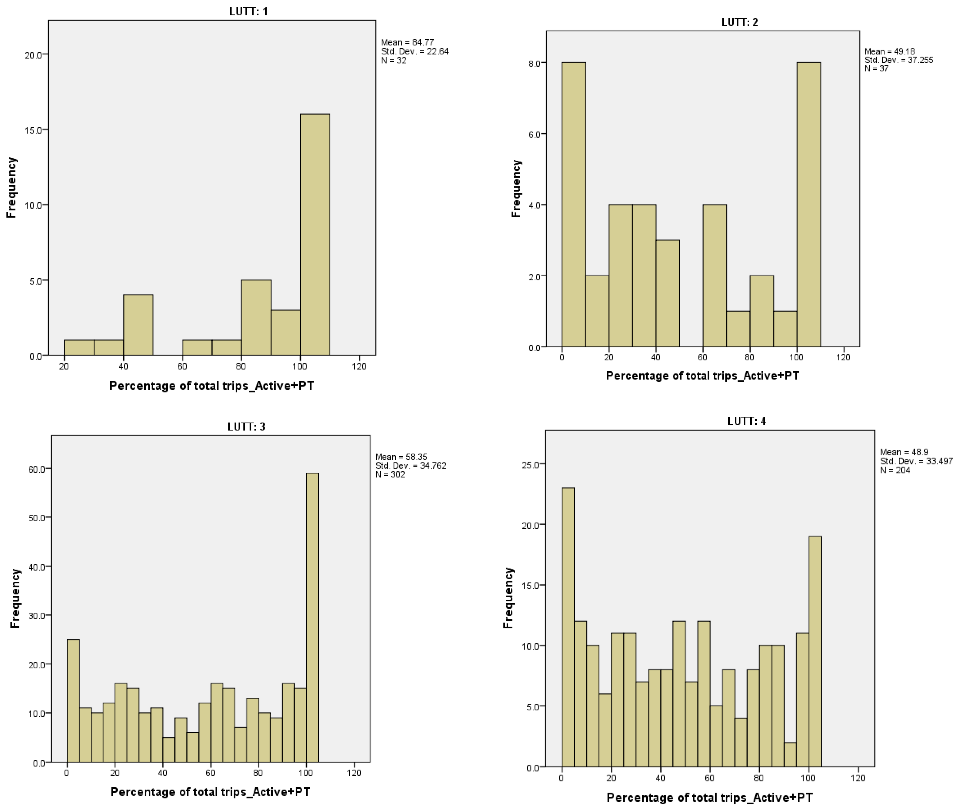
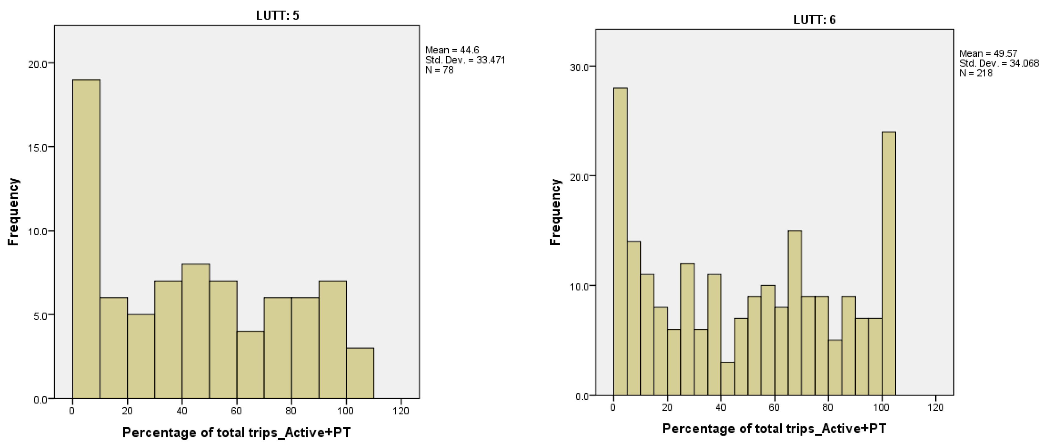
The distribution of responses with respect to the variable Proportion of Total Non-Work trips by Sustainable transport modes is shown in Figure A1.
Figure A1.
Distribution of the Proportion of Total Non-Work Trips using Active and Public Transport Modes in each LUTT.
Figure A1.
Distribution of the Proportion of Total Non-Work Trips using Active and Public Transport Modes in each LUTT.


As shown in Figure A1, none of the distributions showed a normal pattern. Therefore, rather than a one-way ANOVA, a Welch’s ANOVA was applied (for details, see next page). The homogeneity of variances was violated, as assessed by Levene’s Test of Homogeneity of Variance (p = 0.001), and therefore, Welch’s ANOVA is reported. A Kruskall-Wallis test was also applied, but the assumption of similar distributions was not met when all LUTTs were included. The results when LUTT1 and LUTT5 were excluded showed that there were differences in the proportion of all non-work trips by SUST modes across the LUTTs. LUTT 2 (n = 43); LUTT3 (n = 342); LUTT4 (n = 276); LUTT6 (n = 285). The distribution of values was similar across all LUTTs, as assessed by a visual inspection of a boxplot. Median scores were statistically significantly different between groups, H (3) = 36.33, p=0.000. Pairwise comparisons were performed using Dunn’s (1964) procedure, with Bonferroni correction for multiple comparisons. Adjusted p-values are presented. The post hoc analysis revealed statistically significant differences in the mean ranks of the Proportion of Sustainable transport modes used between LUTT 4 (422.87) and LUTT 3 (542.37) (p = 0.000), and LUTT 6 (438.29) and LUTT3 (542.37) (p = 0.000), but not between any other of the pairwise comparisons. Table A2 shows the Mean of the Proportion of Total-Non-Work Trips using sustainable transport modes in each LUTT.
Table A2.
Mean of the Proportion of Total Non-Work Trips using Sustainable Transport Modes (Active and Public transport) in each LUTT.
Table A2.
Mean of the Proportion of Total Non-Work Trips using Sustainable Transport Modes (Active and Public transport) in each LUTT.
| Percentage of Total Trips. _Active+PT | |||
|---|---|---|---|
| UTT | N | Mean | Std. Error |
| 1 | 32 | 84.77 | 4.002 |
| 2 | 37 | 49.18 | 6.125 |
| 3 | 302 | 58.35 | 2.000 |
| 4 | 204 | 48.90 | 2.345 |
| 5 | 78 | 44.60 | 3.790 |
| 6 | 218 | 49.57 | 2.307 |
| Total | 871 | 53.29 | 1.176 |
The results show that there is a statistically significant association between the mean of the proportion of non-work trips using sustainable transport modes and the LUTT of the residence of the respondent. Welch’s F (5, 164.2) = 15.5, p < 0.005. The assumption of normality is necessary for statistical significance testing using a one-way ANOVA. However, the one-way ANOVA is considered “robust” to violations of normality. (See https://statistics.laerd.com/premium/spss/owa/one-way-anova-in-spss-7.php).
This means that some violation of this assumption can be tolerated, and the test will still provide valid results. Therefore, it is often said of this test only requiring approximately normal data. Furthermore, as the sample size increases, the distribution can be very non-normal, and with the Central Limit Theorem, the one-way ANOVA can still provide valid results. Additionally, it should be noted that, if the distributions are all skewed in a similar manner (e.g., all moderately negatively skewed), this is not as troublesome as a situation in which there are groups that have differently-shaped distributions (e.g., the distributions of Group A and Group D are moderately ‘positively’ skewed, while the distributions of Group B and Group C are moderately ‘negatively’ skewed). Therefore, in this example, whether coping stress is normally distributed needs to be investigated.
Note: Technically, it is the residuals (errors) that need to be normally distributed. However, for a one-way ANOVA, the distribution of the scores (observations) in each group will be the same as the distribution of the residuals in each group. However, for a one-way ANOVA, this is equivalent to assuming the normality of the actual scores (observations) in each group (Kirk, 2013).
Appendix C
A multiple regression model was run to determine the influence of income, car ownership, the presence of children, gender, work status and the LUTT on predicting the proportion of the use of the sustainable transport mode (for all trips). Using the Analyze > Generalized Linear Model > Type Linear procedure, the following results were found. Table A3 shows the variables included in the model for the study area.
The model was found to be statistically significant, with the Likelihood Ratio Chi-Square = 311.123, df = 13; p < 0.001 (as shown in Table A4). This shows that the fitted model was statistically significantly a better fit than the intercept-only model (that is, without any of the independent variables). Table A5 shows the Goodness of Fit test statistics for the model.
Table A3.
Categorical Variable Information.
| Categorical Variable Information | ||||
|---|---|---|---|---|
| N | Percent | |||
| Factor | LUTT | 1 | 24 | 3.1% |
| 2 | 31 | 4.0% | ||
| 3 | 225 | 29.0% | ||
| 4 | 188 | 24.2% | ||
| 5 | 117 | 15.1% | ||
| 6 | 191 | 24.6% | ||
| Total | 776 | 100.0% | ||
| Children | No children present | 493 | 63.5% | |
| Children present | 283 | 36.5% | ||
| Total | 776 | 100.0% | ||
| Car ownership level | None | 83 | 10.7% | |
| One | 303 | 39.0% | ||
| Two or more | 390 | 50.3% | ||
| Total | 776 | 100.0% | ||
| Gender_0_Female | Female | 397 | 51.2% | |
| Male | 379 | 48.8% | ||
| Total | 776 | 100.0% | ||
| Work Status | At work | 515 | 66.4% | |
| job seeker, unemployed, student, other, unable to work | 44 | 5.7% | ||
| Home duties | 27 | 3.5% | ||
| Retired | 190 | 24.5% | ||
| Total | 776 | 100.0% | ||
Table A4.
Likelihood Ratio Chi-Square result.
| Omnibus Test a | ||
|---|---|---|
| Likelihood Ratio Chi-Square | df | Sig. |
| 311.123 | 13 | 0.000 |
Dependent Variable: Percentage of total trips_Active+PT. Model: (Intercept), LUTT, Children, B10_carownership, Gender, work status, Income_C4B_NOOUTLIERS_SCALE.
a. Compares the fitted model against the intercept-only model.
Table A5.
Goodness of Fit Tests for the Model.
| Goodness of Fit a | |||
|---|---|---|---|
| Value | df | Value/df | |
| Deviance | 701,245.284 | 762 | 920.269 |
| Scaled Deviance | 776.000 | 762 | |
| Pearson Chi-Square | 701,245.284 | 762 | 920.269 |
| Scaled Pearson Chi-Square | 776.000 | 762 | |
| Log Likelihood b | −3742.003 | ||
| Akaike’s Information Criterion (AIC) | 7514.006 | ||
| Finite Sample Corrected AIC (AICC) | 7514.638 | ||
| Bayesian Information Criterion (BIC) | 7583.818 | ||
| Consistent AIC (CAIC) | 7598.818 | ||
Dependent Variable: Percentage of total trips_Active+PT. Model: (Intercept), LUTT, Children, B10_carownership, Gender, work status, Income_C4B_NOOUTLIERS_SCALE. a. Information criteria are in a small-is-better form. b. The full log likelihood function is displayed and used in computing the information criteria.
Table A6 shows the effects of each independent variable in the model. LUTT and car ownership are statistically significant.
Table A6.
Test of the Model Effects, with Statistically Significant Factors in Bold Text.
| Tests of the Model Effects | |||
|---|---|---|---|
| Source | Type III | ||
| Wald Chi-Square | df | Sig. | |
| (Intercept) | 415.565 | 1 | 0.000 |
| LUTT | 48.261 | 5 | 0.000 |
| Children | 2.009 | 1 | 0.156 |
| B10_carownership | 193.305 | 2 | 0.000 |
| Gender | 4.305 | 1 | 0.038 |
| work status | 5.374 | 3 | 0.146 |
| Income_C4B_NOOUTLIERS_SCALE | 0.155 | 1 | 0.694 |
Dependent Variable: Percentage of total trips_Active+PT. Model: (Intercept), LUTT, Children, B10_carownership, Gender, work_status, Income_C4B_NOOUTLIERS_SCALE.
Table A7 shows the parameter estimates for each level of the categorical independent variables and the one scale variable in the model (income). SPSS creates a dummy variable for every level of a categorical variable, except the last level, which is used as the reference level.
Table A7.
Effects of Each Independent Variable in the Regression Model, with Statistically Significant Factors in Bold Text.
Table A7.
Effects of Each Independent Variable in the Regression Model, with Statistically Significant Factors in Bold Text.
| Parameter Estimates | |||||||
|---|---|---|---|---|---|---|---|
| Parameter | B | Std. Error | 95% Wald Confidence Interval | Hypothesis Test | |||
| Lower | Upper | Wald Chi-Square | df | Sig. | |||
| (Intercept) | 25.072 | 4.2793 | 16.685 | 33.459 | 34.326 | 1 | 0.000 |
| [LUTT = 1] | 21.826 | 6.8096 | 8.480 | 35.173 | 10.273 | 1 | 0.001 |
| [LUTT = 2] | −5.223 | 5.8687 | −16.725 | 6.279 | .792 | 1 | 0.373 |
| [LUTT = 3] | 7.354 | 2.9947 | 1.484 | 13.223 | 6.030 | 1 | 0.014 |
| [LUTT = 4] | −3.280 | 3.1097 | −9.375 | 2.815 | 1.112 | 1 | 0.292 |
| [LUTT = 5] | −13.755 | 3.5757 | −20.764 | −6.747 | 14.799 | 1 | 0.000 |
| [LUTT = 6] | 0 a | . | . | . | . | . | . |
| [Children = 0] | 3.596 | 2.5375 | −1.377 | 8.570 | 2.009 | 1 | 0.156 |
| [Children = 1] | 0 a | . | . | . | . | . | . |
| [B10_carownership = 0] | 55.678 | 4.0231 | 47.793 | 63.563 | 191.536 | 1 | 0.000 |
| [B10_carownership = 1] | 14.856 | 2.4267 | 10.100 | 19.612 | 37.479 | 1 | 0.000 |
| [B10_carownership = 2] | 0 a | . | . | . | . | . | . |
| [Gender = 0] | −4.769 | 2.2984 | −9.274 | −0.264 | 4.305 | 1 | 0.038 |
| [Gender = 1] | 0 a | . | . | . | . | . | . |
| [work_status = 1] | 2.835 | 2.9252 | −2.898 | 8.569 | 0.939 | 1 | 0.332 |
| [work_status = 2] | 10.747 | 5.2595 | 0.439 | 21.055 | 4.175 | 1 | 0.041 |
| [work_status = 3] | 9.571 | 6.5497 | −3.266 | 22.409 | 2.135 | 1 | 0.144 |
| [work_status = 4] | 0 a | . | . | . | . | . | . |
| Income_C4B_NOOUTLIERS_SCALE | 1.491 × 10⁻⁵ | 3.7874 × 10⁻⁵ | −5.932 × 10⁻⁵ | 8.914 × 10⁻⁵ | 0.155 | 1 | 0.694 |
| (Scale) | 903.667 b | 45.8767 | 818.079 | 998.209 | |||
Dependent Variable: Percentage of total trips_Active+PT. Model: (Intercept), LUTT, Children, B10_carownership, Gender, work_status, Income_C4B_NOOUTLIERS_SCALE. a. Set to zero, because this parameter is redundant. b. Maximum likelihood estimate.
Overall, the results indicate that the regression model is statistically significantly a better fit of the dataset than the intercept-only model. The factors that are statistically significant within the model are LUTT and car ownership (both significant at p < 0.001). Considering the parameter estimates in detail, the following interpretation is advanced.
LUTT1 is statistically significant in the model. The proportion of the use of the sustainable transport mode increases substantially in this LUTT1, compared with the reference category of LUTT6 (B = 21.83), p = 0.01. LUTT 3 is statistically significant in the model. The proportion of the use of the sustainable transport mode increases substantially in this LUTT3, compared with LUTT6 (B = 7.354), p = 0.014. LUTT 5 is statistically significant in the model. The proportion of the use of the sustainable transport mode decreases substantially in this LUTT5, compared with LUTT6 (B = −13.75), p < 0.001. Car ownership is statistically significant in this model. The proportion of the use of the sustainable transport mode is much higher among those with no car, compared with those households with 2 or more cars (B = 55.7), p < 0.001. Additionally, for those with one car, there is a higher level of the use of the sustainable transport mode, compared to those with two or more cars (B = 14.856), p < 0.001.
The presence of children, gender, work status and income are not statistically significant in this model.
The coding for each variable is shown in Table A8, and the highest value is the reference value.
Table A8.
Coding for Each Variable.
| Variable Name | Variable Coding | Details |
|---|---|---|
| LUTT | 1–6 | |
| Children | 0 | No children |
| 1 | Children present | |
| Work status | 1 | At work |
| 2 | Job seeker, unemployed, student, other | |
| 3 | Home duties | |
| 4 | Retired | |
| B10_car ownership | 0 | No car |
| 1 | One car | |
| 2 | Two or more cars | |
| Gender | 1 | Female |
| 0 | Male | |
| Income | Per annum |
References
- ITF. International Transport Forum Transport Outlook 2017; OECD Publishing: Paris, France, 2017. [Google Scholar]
- UNECE; WHO. Making THE Link: Transport Choices for our Health, Environment and Prosperity–The Amsterdam Declaration; World Health Organisation Regional Office for Europe: Copenhagen, Denmark, 2009. [Google Scholar]
- WHO. Obesity and Overweight-Fact Sheet Updated June 2016. Available online: https://www.who.int/en/news-room/fact-sheets/detail/obesity-and-overweight (accessed on 23 July 2019).
- Newman, P.W.G.; Kenworthy, J.R. Sustainability and Cities: Overcoming Automobile Dependence; Island Press: Washington, DC, USA, 1999. [Google Scholar]
- Litman, T. Automobile Dependency-Transportation and Land Use Patterns That Cause High Levels of Automobile Use and Reduced Transport Options. Available online: http://www.vtpi.org/tdm/tdm100.htm (accessed on 31 July 2014).
- Handy, S. Methodologies for exploring the link between urban form and travel behaviour. Transp. Res. Part Transp. Environ. 1996, 1, 151–165. [Google Scholar] [CrossRef]
- Ewing, R.; Cervero, R. Does Compact Development Make People Drive Less? The Answer Is Yes. J. Am. Plann. Assoc. 2017, 83, 19–25. [Google Scholar] [CrossRef]
- Handy, S. Thoughts on the Meaning of Mark Stevens’s Meta-Analysis. J. Am. Plann. Assoc. 2017, 83, 26–28. [Google Scholar] [CrossRef]
- Knaap, G.-J.; Avin, U.; Fang, L. Driving and Compact Growth: A Careful Look in the Rearview Mirror. J. Am. Plann. Assoc. 2017, 83, 32–35. [Google Scholar] [CrossRef] [Green Version]
- Stevens, M.R. Does Compact Development Make People Drive Less? J. Am. Plann. Assoc. 2017, 83, 7–18. [Google Scholar] [CrossRef]
- McDonald, N. Household interactions and children’s school travel: The effect of parental work patterns on walking and biking to school. J. Transp. Geogr. 2008, 16, 324–331. [Google Scholar] [CrossRef]
- Dieleman, F.; Dijst, M.; Burghouwt, G. Urban Form and Travel Behaviour: Micro-level Household Attributes and Residential Context. Urban Stud. 2002, 39, 507–527. [Google Scholar] [CrossRef]
- Krizek, K.J. Pretest-Posttest Strategy for Researching Neighborhood-Scale Urban Form and Travel Behaviour. Transp. Res. Rec. 2007, 1722, 48–55. [Google Scholar] [CrossRef]
- Stead, D. Relationships between Land Use, Socioeconomic Factors, and Travel Patterns in Britain. Environ. Plan. B Plan. Des. 2001, 28, 499–528. [Google Scholar] [CrossRef]
- Hanson, S.; Hanson, P. The Travel-Activity Patterns of Urban Residents: Dimensions and Relationships to Sociodemographic Characteristics. Econ. Geogr. 1981, 57, 332–347. [Google Scholar] [CrossRef]
- Bohte, W.; Maat, K.; van Wee, B. Measuring Attitudes in Research on Residential Self-Selection and Travel Behaviour: A Review of Theories and Empirical Research. Transp. Rev. 2009, 29, 325–357. [Google Scholar] [CrossRef]
- Van Acker, V.; Mokhtarian, P.L.; Witlox, F. Car availability explained by the structural relationships between lifestyles, residential location and underlying residential and travel attitudes. Transp. Policy 2014, 35, 88–99. [Google Scholar] [CrossRef]
- Litman, T. Measuring Transportation: Traffic, Mobility and Accessibility. Inst. Transp. Eng. J. 2003, 73, 28–32. [Google Scholar]
- Litman, T.A. Evaluating Accessibility for Transport Planning; Victoria Transport Policy Institute: Victoria, BC, Canada, 2019; p. 63. [Google Scholar]
- Geurs, K.T.; van Wee, B. Accessibility evaluation of land-use and transport strategies: Review and research directions. J. Transp. Geogr. 2004, 12, 127–140. [Google Scholar] [CrossRef]
- Geurs, K.T.; Van Wee, B.; Rietveld, P. Accessibility appraisal of integrated land-use-transport strategies: Methodology and case study for the Netherlands Randstad area. Environ. Plan. B Plan. Des. 2006, 33, 639–660. [Google Scholar] [CrossRef]
- Song, Y.; Merlin, L.; Rodriguez, D. Comparing measures of urban land use mix. Comput. Environ. Urban Syst. 2013, 42, 1–13. [Google Scholar] [CrossRef]
- Fan, Y.; Khattak, A.J. Does urban form matter in solo and joint activity engagement? Landsc. Urban Plan. 2009, 92, 199–209. [Google Scholar] [CrossRef]
- Jones, P. Travel Behaviour: Evolution of Conceptual Framing and Modelling Approaches. Modelling on the Move 7th December 2012; St. Anne’s College: Oxford, UK.
- Handy, S. Transfers Magazine, Pacific Southwest Region University Transportation Center. Available online: http://transfersmagazine.org/wp-content/uploads/sites/13/2018/05/Susan-Handy-_-Enough-with-the-Ds.pdf (accessed on 23 July 2019).
- Mattioli, G. Where Sustainable Transport and Social Exclusion Meet: Households Without Cars and Car Dependence in Great Britain. J. Environ. Policy Plan. 2014, 16, 379–400. [Google Scholar] [CrossRef] [Green Version]
- Boarnet, M.G.; Nesamani, K.S.; Smith, C.S. Comparing the Influence of Land Use on Nonwork Trip Generation and Vehicle Distance Traveled: An Analysis using Travel Diary Data 2003. In Proceedings of the Prepared for the 83rd Annual Meeting of the Transportation Research Board, Washington, DC, USA, 11–15 January 2004. [Google Scholar]
- Gehrke, S.R.; Clifton, K.J. Towards a spatial-temporal measure of land use mix. J. Transp. Land Use 2016, 9, 171–186. [Google Scholar] [CrossRef]
- Song, Y.; Rodriguez, D. The measurement of the level of mixed land uses: A synthetic approach. Carol. Transp. Program White Pap. Ser. Chap. Hill NC 2005.
- Brownson, R.C.; Hoehner, C.; Day, K.; Forsyth, A.; Sallis, J. Measuring the built environment for physical activity: State of the science. Am. J. Prev. Med. 2009, 36, 99–123. [Google Scholar] [CrossRef] [PubMed]
- Rajamani, J.; Bhat, C.; Handy, S.; Knaap, G.; Song, Y. Assessing Impact of Urban Form Measures on Nonwork Trip Mode Choice After Controlling for Demographic and Level-of-Service Effects. Transp. Res. Rec. J. Transp. Res. Board 2003, 1831, 158–165. [Google Scholar] [CrossRef]
- Boarnet, M.G.; Sarmiento, S. Can Land-use Policy Really Affect Travel Behaviour? A Study of the Link between Non-work Travel and Land-use Characteristics. Urban Stud. 1998, 35, 1155–1169. [Google Scholar] [CrossRef]
- European Commission. Directorate General for Mobility and Transport White Paper on Transport: Roadmap to a Single European Transport Area: Towards a Competitive and Resource-Efficient Transport System; Publications Office of the European Union: Luxembourg, Luxembourg, 2011; ISBN 978-92-79-18270-9. [Google Scholar]
- Kenworthy, J. Urban Transport and Eco-Urbanism: A Global Comparative Study of Cities with a Special Focus on Five Larger Swedish Urban Regions. Urban Sci. 2019, 3, 25. [Google Scholar] [CrossRef]
- Department for Transport. Statistics Great Britain 2017. Available online: https://assets.publishing.service.gov.uk/government/uploads/system/uploads/attachment_data/file/661933/tsgb-2017-report-summaries.pdf (accessed on 23 July 2019).
- Department for Transport. Average Distance Travelled by Purpose and Main Mode: England NTS0410. Available online: https://www.gov.uk/government/statistical-data-sets/nts04-purpose-of-trips#trips-stages-distance-and-time-spent-travelling (accessed on 23 July 2019).
- Handy, S. Understanding the Link Between Urban Form and Nonwork Travel Behaviour. J. Plan. Educ. Res. 1996, 15, 183–198. [Google Scholar] [CrossRef]
- Chatman, D.G. Residential choice, the built environment and nonwork travel: Evidence using new data and methods. Environ. Plan. A 2009, 41, 1072–1089. [Google Scholar] [CrossRef]
- Kenworthy, J.R.; Laube, F.B. Patterns of automobile dependence in cities: An international overview of key physical and economic dimensions with some implications for urban policy. Transp. Res. Part Policy Pract. 1999, 33, 691–723. [Google Scholar] [CrossRef]
- Greenwald, M.J.; Boarnet, M.G. The Built Environment as a Determinant of Walking Behaviour: Analyzing Non-Work Pedestrian Travel in Portland, Oregon. Available online: https://escholarship.org/uc/item/9gn7265f (accessed on 23 July 2019).
- Bamberg, S.; Fujii, S.; Friman, M.; Garling, T. Behaviour theory and soft transport policy measures. Transp. Policy 2011, 18, 228–235. [Google Scholar] [CrossRef] [Green Version]
- Sloman, L.; Cairns, S.; Newson, C.; Anable, J.; Pridmore, A.; Goodwin, P. The Effects of Smarter Choice Programmes in the Sustainable Travel Towns: Summary Report. Available online: https://webarchive.nationalarchives.gov.uk/20120208112937/http://www.dft.gov.uk/publications/the-effects-of-smarter-choice-programmes-in-the-sustainable-travel-towns-summary-report/ (accessed on 23 July 2019).
- Cairns, S.; Sloman, L.; Newson, C.; Anable, J.; Kirkbride, A.; Goodwin, P. Smarter Choices: Assessing the Potential to Achieve Traffic Reduction Using ‘Soft Measures.’. Transp. Rev. 2008, 28, 593–618. [Google Scholar] [CrossRef]
- Buehler, R. Determinants of transport mode choice: A comparison of Germany and the USA. J. Transp. Geogr. 2011, 644–657. [Google Scholar] [CrossRef]
- Susilo, Y.O.; Williams, K.; Lindsay, M.; Dair, C. The influence of individuals’ environmental attitudes and urban design features on their travel patterns in sustainable neighborhoods in the UK. Transp. Res. Part Transp. Environ. 2012, 17, 190–200. [Google Scholar] [CrossRef]
- Central Statistics Office. National Travel Survey 2009; Stationery Office: Dublin, Ireland, 2011; ISBN 978-1-4064-2552-9. [Google Scholar]
- Central Statistics Office Census of Population 2016 2018. Available online: https://www.cso.ie/en/census/ (accessed on 23 July 2019).
- Kelobonye, K.; Xia, J.C.; Swapan, M.S.H.; McCarney, G.; Zhou, H. Drivers of Change in Urban Growth Patterns: A Transport Perspective from Perth, Western Australia. Urban Sci. 2019, 3, 40. [Google Scholar] [CrossRef]
- National Transport Authority. Transport Strategy for the Greater Dublin Area 2016–2035; National Transport Authority: Dublin, Ireland, 2016. [Google Scholar]
- Hennig, E.I.; Schwick, C.; Soukup, T.; Orlitová, E.; Kienast, F.; Jaeger, J.A.G. Multi-scale analysis of urban sprawl in Europe: Towards a European de-sprawling strategy. Land Use Policy 2015, 49, 483–498. [Google Scholar] [CrossRef] [Green Version]
- Graby, J.; Meghen, K. The New Housing; Gandon Press in Association with the RIAI and the Department of the Environment and Local Government; Gandon Press: Cork, Ireland, 2002. [Google Scholar]
- Robinson, J.W. Dutch complex housing: Design for density. In Proceedings of the Future of Architectural Research ARCC 2015, Chicago, IL, USA, 6–9 April 2015. [Google Scholar]
- Van, U.-P.; Senior, M. The Contribution of Mixed Land Uses to Sustainable Travel in Cities. In Achieving Sustainable Urban Form; Williams, K., Burton, E., Jenks, M., Eds.; E & FN Spon: London, UK, 2000. [Google Scholar]
- Cardiff Council. Cardiff Residential Design Guide Supplementary Planning Guidance 2017; Cardiff Council: Cardiff, Wales, 2017. [Google Scholar]
- Bartlett, J.E.; Kotrllik, J.W.; Higgins, C.C. Organizational research: Determining appropriate sample size in survey research appropriate sample size in survey research. Inf. Technol. Learn. Perform. J. 2001, 19, 43. [Google Scholar]
- Field, A. Discovering Statistics Using IBM SPSS Statistics, 4th ed.; Sage Publications: London, UK, 2013. [Google Scholar]
- Gravetter, F.J.; Wallnau, L.B. Statistics for the Behavioural Sciences, 8th ed.; Wadsworth CENGAGE Learning: Belmont, CA, USA, 2009. [Google Scholar]
- Central Statistics Office Census of Population 2011 2012. Available online: https://www.cso.ie/en/census/ (accessed on 23 July 2019).
- Convery, S.; Williams, B. Exploring Determinants of Mode Choice for Non-Work Travel in the Greater Dublin Region. In Proceedings of the ITRN2016, Dublin Institute of Technology, Grangegorman, Dublin, Ireland, 1–2 September 2016. [Google Scholar]
- How far do People Walk? Presented at the PTRC Transport Practitioners’ Meeting London, July 2015. Available online: https://www.wyg.com/uploads/files/news/WYG_how-far-do-people-walk.pdf (accessed on 23 July 2019).
- Grist, B. An Introduction to Irish Planning Law, 2nd ed.; Institute of Public Administration: Dublin, Ireland, 2012. [Google Scholar]
- Cohen, J. Statistical Power Analysis for the Behavioural Sciences; Lawrence Erlbaum Associates: Hillsdale, NJ, USA, 1988. [Google Scholar]
- Laerd Statistics One-Way ANOVA using SPSS Statistics. Statistical Tutorials and Software Guides. 2017. Available online: https://statistics.laerd.com/ (accessed on 23 July 2019).
- Pallant, J. SPSS Survival Manual A Step by Step Guide to Data Analysis Using SPSS, 4th ed.; McGraw Hill Education: Maidenhead, UK, 2010. [Google Scholar]
- Gerring, J. Description and Prediction. In A Criterial Framework; Cambridge University Press: Cambridge, UK, 2001. [Google Scholar]
- Potoglou, D.; Kanaroglou, P.S. Modelling car ownership in urban areas: a case study of Hamilton, Canada. J. Transp. Geogr. 2008, 16, 42–54. [Google Scholar] [CrossRef]
- Humphreys, J.; Ahern, A. Is travel based residential self-selection a significant influence in modal choice and household location decisions? Transp. Policy 2017, 75, 150–160. [Google Scholar] [CrossRef]
- Sommer, B.; Sommer, R. A Practical Guide to Behavioural Research: Tools and Techniques, 4th ed.; Oxford University Press: Oxford and New York, NY, USA, 1997. [Google Scholar]
Figure 1.
The Greater Dublin Region.

Figure 2.
Map of the Greater Dublin Region, Ireland, showing the 6 typologies of land-use transport characteristics. The INSET shows the core city centre area, which is mostly type 3 and where all the type 1 areas are located.
Figure 2.
Map of the Greater Dublin Region, Ireland, showing the 6 typologies of land-use transport characteristics. The INSET shows the core city centre area, which is mostly type 3 and where all the type 1 areas are located.

Table 1.
Description of Six Land Use–Transport Typologies, showing Key Selection Criteria.
| Very High Residential Density | Medium Residential Density | Low Residential Density | |||||
|---|---|---|---|---|---|---|---|
| Criteria | Measure | LUTT 1 | LUTT 2 | LUTT 3 | LUTT 4 | LUTT 5 | LUTT 6 |
| Residential Density | Dwelling per hectare | Greater than 240 | Between 55 and 240 | Between 55 and 240 | Between 55 and 240 | Less than 55 | Less than 55 |
| Accessibility | Proximity to public transport network * and frequency of service ** | High | Various | Medium | Low | Low | Low |
| Proximity to retail cluster | Within 1 km of a retail cluster (>35 retail units per hectare) | Yes | Various | Yes | Yes | No | No |
| Planning Designation | Strategic Development Zone (SDZ) | No | Yes | No | No | No | No |
* Within 500 m of a bus stop and/or 1 km of a LUAS or train stop. ** Frequency of service: Low = 0–2 services per hour; Medium = 3–4 per hour; High = 5–6 per hour (using the reference hour between 3pm and 4pm on a weekday).
Table 2.
Key Socio-Demographic Characteristics of each LUTT.
| Socio-Demographic | Very High Res. Dens. | Medium Residential Density | Low Residential Density | ||||
|---|---|---|---|---|---|---|---|
| Description | Unit | LUTT 1 | LUTT 2 | LUTT 3 | LUTT 4 | LUTT 5 | LUTT 6 |
| Average Household Size | Total Population/Number Occupied Housing Units | 2.03 | 2.79 | 2.56 | 2.81 | 2.96 | 2.82 |
| Population | Number of Small Areas * | 40 | 108 | 1771 | 1415 | 1099 | 1276 |
| Persons | 9079 | 30,492 | 431,175 | 390,851 | 311,044 | 353,698 | |
LUTT 1–6 are mutually exclusive, i.e., no small area can appear in more than one area type. * Small Areas are areas of population comprising between 50 and 200 dwellings, and, situated at the lowest level of geography for the compilation of statistics in line with data protection, they are nested inside electoral divisions. All population figures are taken from the CSO, 2011 and Geodirectory 2013.
Table 3.
Interpretation of the Effect Size Values r2.
| Percentage of Variance Explained, r2 | ||
|---|---|---|
| r2 | 0.01 | Small effect |
| 0.09 | Medium effect | |
| 0.25 | Large effect | |
Source: [57].
Table 4.
Strength of the Association between the Mode Use (proportion) and the Land Use–Transport Type (LUTT) [Cramér’s V].
Table 4.
Strength of the Association between the Mode Use (proportion) and the Land Use–Transport Type (LUTT) [Cramér’s V].
| Land Use–Transport Type | ||||||||||
|---|---|---|---|---|---|---|---|---|---|---|
| Trip Purpose | Mode | 1 | 2 | 3 | 4 | 5 | 6 | TOTAL Respondents (N) | Chi Square | Cramér’s V |
| Pharmacy | Car | 0.07 | 0.49 | 0.3 | 0.55 | 0.69 | 0.49 | 1245 | 115.16 ** | 0.304 |
| Sust | 0.93 | 0.51 | 0.7 | 0.45 | 0.31 | 0.51 | ||||
| GP | Car | 0.17 | 0.59 | 0.48 | 0.65 | 0.86 | 0.65 | 1216 | 108.46 ** | 0.299 |
| Sust | 0.83 | 0.41 | 0.52 | 0.35 | 0.14 | 0.35 | ||||
| INTREO” | Car | 0.08 | 0.91 | 0.38 | 0.58 | 0.88 | 0.67 | 289 | 53.13 ** | 0.429 |
| Sust | 0.92 | 0.09 | 0.62 | 0.42 | 0.12 | 0.33 | ||||
| PO | Car | 0.02 | 0.49 | 0.3 | 0.48 | 0.7 | 0.44 | 1180 | 107.27 ** | 0.302 |
| Sust | 0.98 | 0.51 | 0.7 | 0.52 | 0.3 | 0.56 | ||||
| SPORTS | Car | 0.2 | 0.74 | 0.6 | 0.8 | 0.91 | 0.76 | 614 | 70.05 ** | 0.338 |
| Sust | 0.8 | 0.26 | 0.4 | 0.2 | 0.09 | 0.24 | ||||
| SWIM | Car | 0.24 | 0.9 | 0.66 | 0.81 | 0.96 | 0.84 | 600 | 73.18 ** | 0.349 |
| Sust | 0.76 | 0.1 | 0.34 | 0.19 | 0.04 | 0.16 | ||||
| CINEMA | Car | 0.13 | 0.77 | 0.54 | 0.8 | 0.98 | 0.84 | 983 | 182.47 ** | 0.431 |
| Sust | 0.87 | 0.23 | 0.46 | 0.2 | 0.02 | 0.16 | ||||
| THEATRE | Car | 0.03 | 0.69 | 0.39 | 0.66 | 0.89 | 0.65 | 812 | 126.97 ** | 0.395 |
| Sust | 0.97 | 0.31 | 0.61 | 0.34 | 0.11 | 0.35 | ||||
| SOCIAL | Car | 0.15 | 0.75 | 0.5 | 0.73 | 0.85 | 0.7 | 441 | 44.85 ** | 0.319 |
| Sust | 0.85 | 0.25 | 0.5 | 0.27 | 0.15 | 0.3 | ||||
| WORSHIP | Car | 0.41 | 0.76 | 0.49 | 0.58 | 0.78 | 0.59 | 891 | 39.19 ** | 0.21 |
| Sust | 0.59 | 0.24 | 0.51 | 0.42 | 0.22 | 0.41 | ||||
| FAMILY & FRIENDS | Car | 0.4 | 0.71 | 0.68 | 0.82 | 0.91 | 0.83 | 1165 | 78.41 ** | 0.259 |
| Sust | 0.6 | 0.29 | 0.32 | 0.18 | 0.09 | 0.17 | ||||
| ATTEND A CLASS | Car | 0.18 | 0.72 | 0.51 | 0.73 | 0.87 | 0.71 | 596 | 68.07 ** | 0.338 |
| Sust | 0.82 | 0.28 | 0.49 | 0.27 | 0.13 | 0.29 | ||||
| LOCAL SHOP | Car | 0.05 | 0.42 | 0.27 | 0.46 | 0.66 | 0.46 | 1182 | 102.68 ** | 0.295 |
| Sust | 0.95 | 0.58 | 0.73 | 0.54 | 0.34 | 0.54 | ||||
| SUPERMARKET SHOP | Car | 0.33 | 0.7 | 0.69 | 0.82 | 0.94 | 0.84 | 1217 | 103.38 ** | 0.291 |
| Sust | 0.67 | 0.3 | 0.31 | 0.18 | 0.06 | 0.16 | ||||
Note: “2 cells have an expected count of less than 5. The min. expected count is 4.42. Not all respondents provided an answer for each destination, which is why the number of respondents is different for each destination type. The smallest response was for the destination, INTREO (Social Welfare office), while the highest response was for the pharmacy, with 1245 out of 1298 providing a response to this question. ** p < 0.001
Table 5.
Mode Split by Journey Purpose: Non-Work Destinations.
| Destination | Active | Car | Public Transport | Other | N |
|---|---|---|---|---|---|
| Pharmacy 3 | 52.4% 3 | 43.8% | 1.4% | 2.4% | 1248 |
| GP 3 | 33.2% 3 | 56.7% | 5.7% | 4.4% | 1219 |
| Social Welfare (INTREO) | 31.6% | 54.6% | 8.6% | 5.2% | 291 |
| Post Office 3 | 54.4% 3 | 41.1% | 2.5% | 2.0% | 1183 |
| Sports Centre 1 | 24.6% | 69.2% 1 | 2.9% | 3.3% | 614 |
| Swimming Pool 1 | 18.6% | 72.4% 1 | 3.2% | 5.8% | 602 |
| Cinema 2 | 15.4% | 63.9% | 11.9% 2 | 8.8% | 986 |
| Theatre 2 | 10.2% | 49.0% | 32.4% 2 | 8.4% | 814 |
| Social club 2 | 23.8% | 58.7% | 10.7% 2 | 6.8% | 441 |
| Place of worship | 38.6% | 52.5% | 2.2% | 6.7% | 892 |
| Friends and family visit 1 | 12.8% | 70.2% 1 | 9.6% 2 | 7.4% | 1168 |
| Class attendance 2 | 21.1% | 62.4% | 13.0% 2 | 3.5% | 598 |
| Local shop 3 | 57.0% 3 | 40.1% | 1.4% | 1.5% | 1185 |
| Supermarket 1 | 17.8% | 72.5% 1 | 4.1% | 5.7% | 1220 |
Note: 1 Highest share of car use; 2 Highest share of public transport; 3 Highest share of active transport.
Table 6.
Mean and Ns for the LUTTS included in the Welch’s ANOVA analysis.
| Proportion of Total Trips by Sustainable Transport Modes (Active and PT) | |||
|---|---|---|---|
| N | Mean | Std. Deviation | |
| 1 | 32 | 84.77 | 22.640 |
| 2 | 37 | 49.18 | 37.255 |
| 3 | 302 | 58.35 | 34.762 |
| 4 | 204 | 48.90 | 33.497 |
| 5 | 78 | 44.60 | 33.471 |
| 6 | 218 | 49.57 | 34.068 |
| Total | 871 | 53.29 | 34.714 |
Table 7.
Mean and Standard Errors (Games-Howell).
| Multiple Comparisons | |||||
|---|---|---|---|---|---|
| Dependent Variable: Percentage of Total Trips_Active + PT | |||||
| LUTT | Mean Difference | Std. Error | Sig. | 95% Confidence Interval | |
| Lower Bound | Upper Bound | ||||
| 1–2 | 35.586 * | 7.316 | p < 0.001 | 14.05 | 57.12 |
| 1–3 | 26.412 * | 4.474 | p < 0.001 | 13.13 | 39.69 |
| 1–4 | 35.869 * | 4.639 | p < 0.001 | 22.17 | 49.57 |
| 1–5 | 40.170 * | 5.512 | p < 0.001 | 24.10 | 56.24 |
| 1–6 | 35.198 * | 4.620 | p < 0.001 | 21.55 | 48.85 |
| 3–4 | 9.457 ** | 3.082 | 0.01< p < 0.05 | 0.63 | 18.28 |
| 3–5 | 13.758 ** | 4.285 | 0.01 < p < 0.05 | 1.35 | 26.16 |
| 3–6 | 8.786 ** | 3.054 | 0.01 < p < 0.05 | 0.05 | 17.52 |
Significance values and confidence intervals for the mean of the proportion of total non-work trips reached by active and PT modes, when comparing the LUTTs. * p < 0.001, ** 0.01 < p < 0.05
Table 8.
Parameter Estimates for the Model, with Significant Values shown in Bold Text.
| Parameter Estimates | |||||||
|---|---|---|---|---|---|---|---|
| Parameter | B | Std. Error | 95% Wald Confidence Interval | Hypothesis Test | |||
| Lower | Upper | Wald Chi-Square | df | Sig. | |||
| Intercept | 25.072 | 4.2793 | 16.685 | 33.459 | 34.326 | 1 | 0.000 |
| LUTT1 | 21.826 | 6.8096 | 8.480 | 35.173 | 10.273 | 1 | 0.001 |
| LUTT2 | –5.223 | 5.8687 | –16.725 | 6.279 | 0.792 | 1 | 0.373 |
| LUTT3 | 7.354 | 2.9947 | 1.484 | 13.223 | 6.030 | 1 | 0.014 |
| LUTT4 | 3.280 | 3.1097 | –9.375 | 2.815 | 1.112 | 1 | 0.292 |
| LUTT5 | –13.755 | 3.5757 | –20.764 | –6.747 | 14.799 | 1 | 0.000 |
| LUTT6 | 0 a | . | . | . | . | . | . |
| Children Not Present | 3.596 | 2.5375 | –1.377 | 8.570 | 2.009 | 1 | 0.156 |
| Car ownership 0 | 55.678 | 4.0231 | 47.793 | 63.563 | 191.536 | 1 | 0.000 |
| Car ownership 1 | 14.856 | 2.4267 | 10.100 | 19.612 | 37.479 | 1 | 0.000 |
| Gender Male | –4.769 | 2.2984 | –9.274 | –.264 | 4.305 | 1 | 0.038 |
| Job seeker/Student | 2.835 | 2.9252 | –2.898 | 8.569 | 0.939 | 1 | 0.332 |
| At work | 10.747 | 5.2595 | 0.439 | 21.055 | 4.175 | 1 | 0.041 |
| Home duties | 9.571 | 6.5497 | –3.266 | 22.409 | 2.135 | 1 | 0.144 |
| Retired | 0 a | . | . | . | . | . | . |
| Income | 1.491 × 10⁻⁵ | 3.7874 × 10⁻⁵ | –5.932 × 10⁻⁵ | 8.914 × 10⁻⁵ | 0.155 | 1 | 0.694 |
| (Scale) | 903.667 b | 45.8767 | 818.079 | 998.209 | |||
Dependent Variable: Percentage of total trips_Active+PT. Model: (Intercept), LUTT, Children, B10_carownership, Gender, work status, Income_C4B_NOOUTLIERS_SCALE. a Set to zero, because this parameter is redundant. b Maximum likelihood estimate.
Table 9.
Relationship Between Income, Car Ownership and the Proportion of the Use of the Sustainable Transport Mode and the Total Number of Non-Work Trips (annual basis).
Table 9.
Relationship Between Income, Car Ownership and the Proportion of the Use of the Sustainable Transport Mode and the Total Number of Non-Work Trips (annual basis).
| Variable | Correlation Coefficient | p Value | N | ||
|---|---|---|---|---|---|
| Income | Car Ownership | 0.215 | Spearman’s rho | <0.001 | 957 |
| Proportion of the use of the sustainable transport mode | −0.069 | Pearson r | <0.05 | 854 | |
| Proportion of the use of the sustainable transport mode 1 | −0.096 | Pearson r | <0.05 | 654 | |
| Total number of non-work trips (activity level) | 0.012 | Pearson r | n.s. | 959 | |
| Total number of non-work trips (activity level) 2 | −0.043 | Pearson r | n.s. | 854 | |
1 Not including cases, where the Proportion = 0. 2 Not including cases, where the total number of trips = 0.
© 2019 by the authors. Licensee MDPI, Basel, Switzerland. This article is an open access article distributed under the terms and conditions of the Creative Commons Attribution (CC BY) license (http://creativecommons.org/licenses/by/4.0/).
Share and Cite
MDPI and ACS Style
Convery, S.; Williams, B. Determinants of Transport Mode Choice for Non-Commuting Trips: The Roles of Transport, Land Use and Socio-Demographic Characteristics. Urban Sci. 2019, 3, 82. https://doi.org/10.3390/urbansci3030082
AMA Style
Convery S, Williams B. Determinants of Transport Mode Choice for Non-Commuting Trips: The Roles of Transport, Land Use and Socio-Demographic Characteristics. Urban Science. 2019; 3(3):82. https://doi.org/10.3390/urbansci3030082
Chicago/Turabian StyleConvery, Sheila, and Brendan Williams. 2019. "Determinants of Transport Mode Choice for Non-Commuting Trips: The Roles of Transport, Land Use and Socio-Demographic Characteristics" Urban Science 3, no. 3: 82. https://doi.org/10.3390/urbansci3030082