
Field-Deployable Fiber Optic Sensor System for Structural Health Monitoring of Steel Girder Highway Bridges


1
Department of Civil and Architectural Engineering, University of Wyoming, 1000 E. University Ave., Laramie, WY 82071, USA
2
Department of Civil and Construction Engineering, Brigham Young University, 430 Engineering Building, Provo, UT 84602, USA
*
Author to whom correspondence should be addressed.
Infrastructures 2022, 7(2), 16; https://doi.org/10.3390/infrastructures7020016
Submission received: 4 January 2022
/
Revised: 12 January 2022
/
Accepted: 24 January 2022
/
Published: 26 January 2022
(This article belongs to the Special Issue Structural Health Monitoring of Civil Infrastructures)
Abstract
:Structural health monitoring of highway bridges is a vital but currently challenging aspect of infrastructure engineering due to the number of sensors required, power requirements, and harsh environmental conditions. The purpose of this study is to develop a structural health monitoring system using fiber optic sensors based on fiber Bragg gratings that addresses these issues and is field deployable. Prototype systems were installed on two steel girder bridges. The first bridge used sensors adhered to the web and flange. The second bridge used a flange-only array of mechanically mounted sensors. The results demonstrated the accuracy of the fiber Bragg grating sensors and indicated that fewer multiplexed fiber optic cables and loosely routed cables were needed to maintain signal integrity. Adhered sensors were prone to lose their bond due to the curing conditions in the field. The findings suggest that the proposed system may be best used in a hybrid deployment, where a diagnostic field test with conventional sensors is used to determine the baseline bridge response and fiber optic sensors are periodically installed for short-term monitoring.
1. Introduction
The condition of highway bridges is one of the most well-known indicators of the overall health of civil infrastructure [1]. Furthermore, a recent study estimated that 30% of the bridges in the USA are over 50 years old, and of these bridges, 11% are structurally deficient [2]. However, the number of deficient bridges is likely higher because the estimate in that study was based on the National Bridge Inventory (NBI) database, which does not consider vehicular bridges with spans shorter than 6 m (20 ft). Furthermore, the NBI database employed some visual-only inspections, and it is possible that had these inspections employed instrumentation, additional bridges would be identified as deficient.
Structural deterioration of bridges can be caused by a variety of natural or anthropogenic sources. Some of the primary natural sources include hydrodynamic pressures, scouring of bridges, and seismicity. The risk of deterioration from natural hazards is a function of both the bridge’s vulnerability and the time that the bridge is exposed to the hazards. It follows that the structural condition of existing older bridges is therefore particularly important. Anthropogenic sources of deterioration include increased traffic, fatigue due to traffic, and overweight vehicles. Overweight vehicles are particularly important in regions where heavy machinery and equipment (e.g., equipment for the energy sector or military needs) are routinely transported over surface roads. In these cases, the bridges are potentially subjected to vehicular loads that are well above the safe load carrying capacity of the structure. Thus, both evaluating and monitoring the structural condition of highway bridges (“structural health monitoring”) has become a desired approach to address deficiencies and allocate maintenance resources [3,4].
Structural health monitoring systems can be classified as having one or more of the following objectives: sensor deployment, anomaly detection, model validation, threshold check, and damage detection [5]. The types of data measured in a typical structural health monitoring system are summarized in Modares and Waksmanski [6]. The main types are cracking, displacement, settlement, tilt, vibration, and strain. In a holistic effort to assess performance [7], the measured data collected in the structural health monitoring can be augmented with visual inspections, diagnostic field testing, and analytical models. For bridges, structural health monitoring systems have also been used to determine natural frequencies [8], assess the condition of the substructure [9], and detect other damage [10].
Structural health monitoring systems consist of the following basic components: sensors (e.g., to measure strain), a sensor excitation hardware system, a host computer, communication hardware, and software components, e.g., [6,11]. Among these, the central component is the sensor. Fiber optic sensors have several advantages compared to other types of sensors. Fiber optic sensors are immune to electromagnetic interference. They are small, and the cabling is lightweight. The electrical power required is relatively low, e.g., [12,13,14]. The main disadvantages of fiber optic sensors are that they tend to be less sturdy and the cables less durable, compared to conventional sensors [15]. The glass fiber also expands and contracts with temperature variations [4]. To address these issues, fiber optic sensors are often embedded [16] and/or housed in protective cases [17,18].
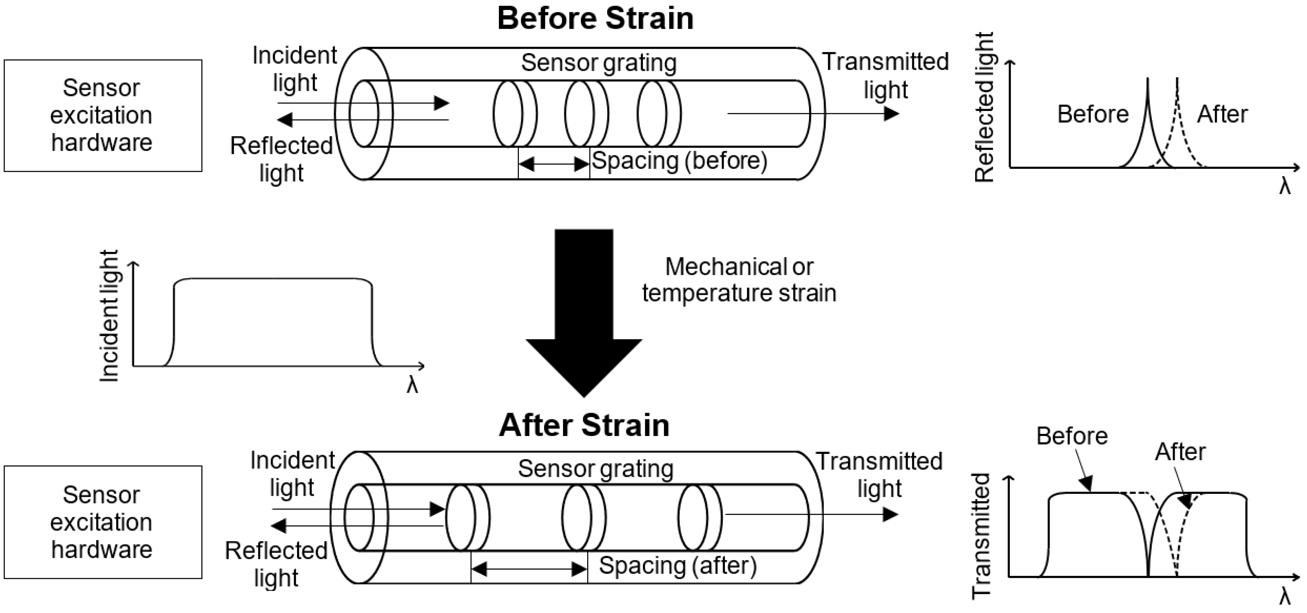
There are two main types of fiber optic sensors for measuring strain: distributed sensors, e.g., [13,19] and discrete sensors using fiber Bragg gratings, e.g., [12], which are the focus of this study. Figure 1 shows how a fiber Bragg grating sensor works. In a fiber Bragg grating sensor, the core of the fiber is etched so that selected wavelengths of light are reflected, and other wavelengths are transmitted. When the fiber is subjected to strain, the spacing of the Bragg gratings change. This change in spacing causes a shift in the reflected wavelength. The change in wavelength can then be correlated to the applied strain.
A valuable feature of fiber Bragg grating sensors is that multiple sensors can be used on a single fiber optic line (i.e., the fiber can be multiplexed) by controlling the grating spacing so that each sensor has a unique central wavelength, e.g., [20]. In this way, fiber optic structural health monitoring systems have the potential to require less cabling compared to equivalent conventional sensor systems, which require dedicated cables for each sensor.
Fiber optic structural health monitoring systems have been developed for many elements of civil infrastructure, such as levees, dams [21], pipelines and wind turbines [22], tunnels [23], and bridges [24]. Although several prior studies have examined the application of fiber optic structural health monitoring systems for bridges, the focus of these studies has been mainly on permanently installed systems. For example, fiber optic systems were installed on the Honxing Bridge in Wuxi, China [17], the Trezói Bridge in Covilhã, Portugal [25], the Mile 17.7 Grimsby Railway Bridge in Ontario, Canada [26], a bridge in North Yorkshire, UK [27], the Mjosund Bridge in western Norway [28], and a bridge in Iowa, USA [29]. With the exception of the fiber optic sensors installed on the Iowa bridge, which were later removed and replaced with conventional strain gages because the fiber optic system was not considered as robust or cost-effective [30], in each of the studies cited here, the structural health monitoring system was intended to be permanent. To the authors’ knowledge, only two nonpermanent systems have been developed to date: one for a reinforced concrete girder bridge [19], and another for levees [31].
The overarching goal of this research effort is to develop a robust fiber optic structural health monitoring system for steel girder highway bridges that can be deployed in the field, and then removed as needed. In this phase of the research, the emphasis is on the configuration of the sensor array and method used to attach the sensor to the girders. Other aspects of the system (e.g., remote data collection and postprocessing of data) are beyond the scope of this phase but will be addressed in a subsequent phase.
2. Materials and Methods
To achieve the research goal, laboratory tests were conducted to develop methods to mount and to protect distributed and discrete fiber optic strain sensors to concrete girders [32,33] and steel girders [34]. The tests for steel girders indicated that the strain sensors were sensitive to various factors, in particular the orientation of the sensor (i.e., along the axis of the member) and the interaction between major-axis and minor-axis bending. Based on these results, a discrete fiber optic system was selected. The system was then installed on two highway bridges that have cross frames that minimize biaxial bending. The bridges are described in detail in the next section.
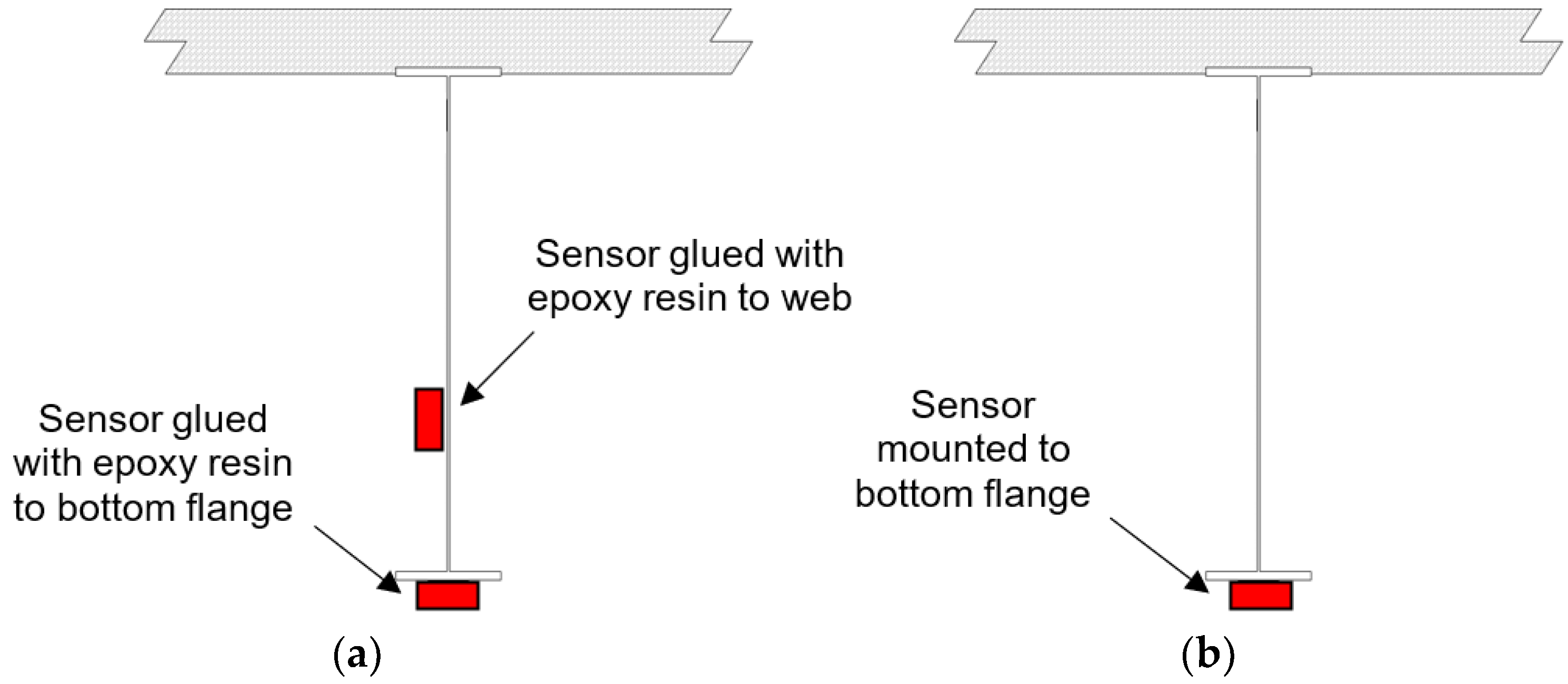
Two fiber optic sensor configurations, shown in Figure 2, were evaluated. The first configuration was a web-and-flange array. In this configuration, the fiber optic sensors were glued with epoxy resin to the girder web and flange. Two sensors were used so that the strain profiles of the girders could be determined for elastic loads. To validate the prototype system, conventional strain transducer sensors were also installed parallel to the fiber optic sensors, and a diagnostic field test was conducted. The second configuration was a flange-only array. In this configuration, the fiber optic sensors were mechanically mounted to the bottom flange. A diagnostic field test was used to determine the girder strain profiles.
3. Web-and-Flange Array Configuration
3.1. Bridge Description
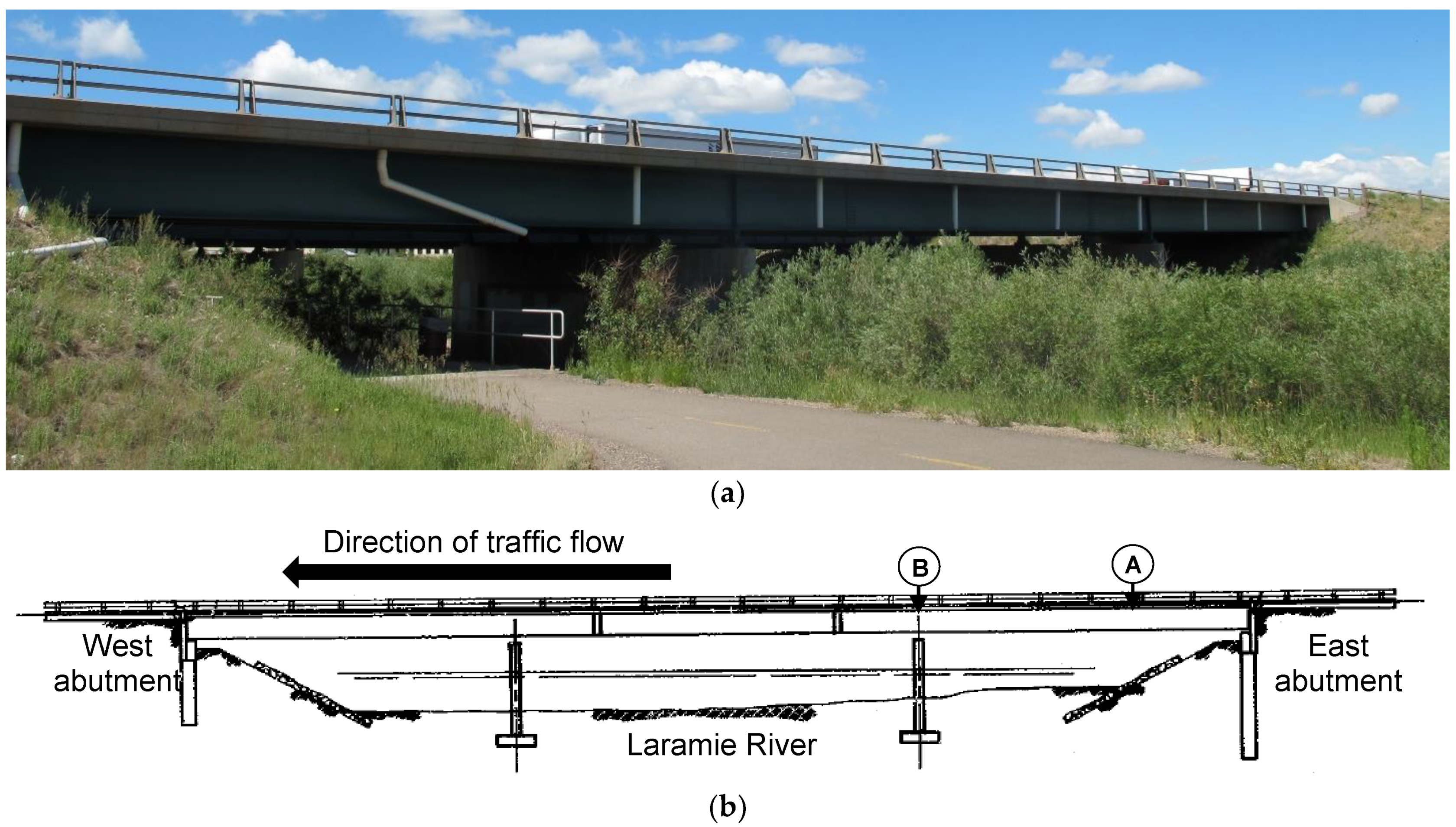
The web-and-flange array configuration was installed on the westbound bridge on Interstate 80 over the Laramie River in Laramie, Wyoming, USA. The bridge is shown in Figure 3. This bridge was selected for the study, because it was accessible without a snooper truck. The bridge is a symmetric non-composite continuous bridge and consists of three spans: 18.3 m (60 ft) for the outer spans and 22.9 m (75 ft) for the inner span. The bridge deck is supported by five I-shape bisymmetrical steel plate girders. The bridge was originally constructed with four girders (Girders 1–4) and then later widened by adding a fifth girder (Girder 5). The widened section of the bridge uses a concrete slab on a metal deck between the two most northern girders.
The clear roadway width of the bridge is approximately 12.2 m (40 ft) with a 0.41-m (16-in.) curb on each side. The spacing between the original girders is 2.69 m (8 ft 10 in.), and the spacing between the girder, added after widening, and the adjacent original girder is 2.74 m (9 ft). The deck has a thickness of 191 mm (7.5 in.) plus an overlay of 25.4 mm (1 in.) throughout the whole bridge. Girders are supported by a fixed bearing at one abutment and by expansion bearings at the other abutment and at interior piers.
The dimensions of the girders at selected locations shown in Figure 3 are given in Table 1. The girder top flange is fully embedded in the deck. Both flange and web are thicker at the pier for the original girders, but the added girder (Girder 5) has a constant thickness. The original girders were specified to be 228 MPa (33 ksi) structural steel. The concrete of the corresponding deck has a specified (nominal) compressive strength equal to 22.4 MPa (3250 psi) with Grade 40 reinforcing steel. The fifth girder was specified to be 345 MPa (50 ksi) structural steel, and the concrete for the widened section has a specified (nominal) compressive strength equal to 25.9 MPa (3750 psi) with Grade 60 reinforcing steel. Cross bracing frames are present in each span. The cross frames are spaced every 6.10 m (20 ft) in the outer spans and 7.62 m (25 ft) in the inner span. The girders contain two field splices in the inner span located 4.57 m (15 ft) from the interior support (pier). There are two girder splices in the outer spans located 12.8 m (42 ft) from the abutment.
3.2. Fiber Optic System
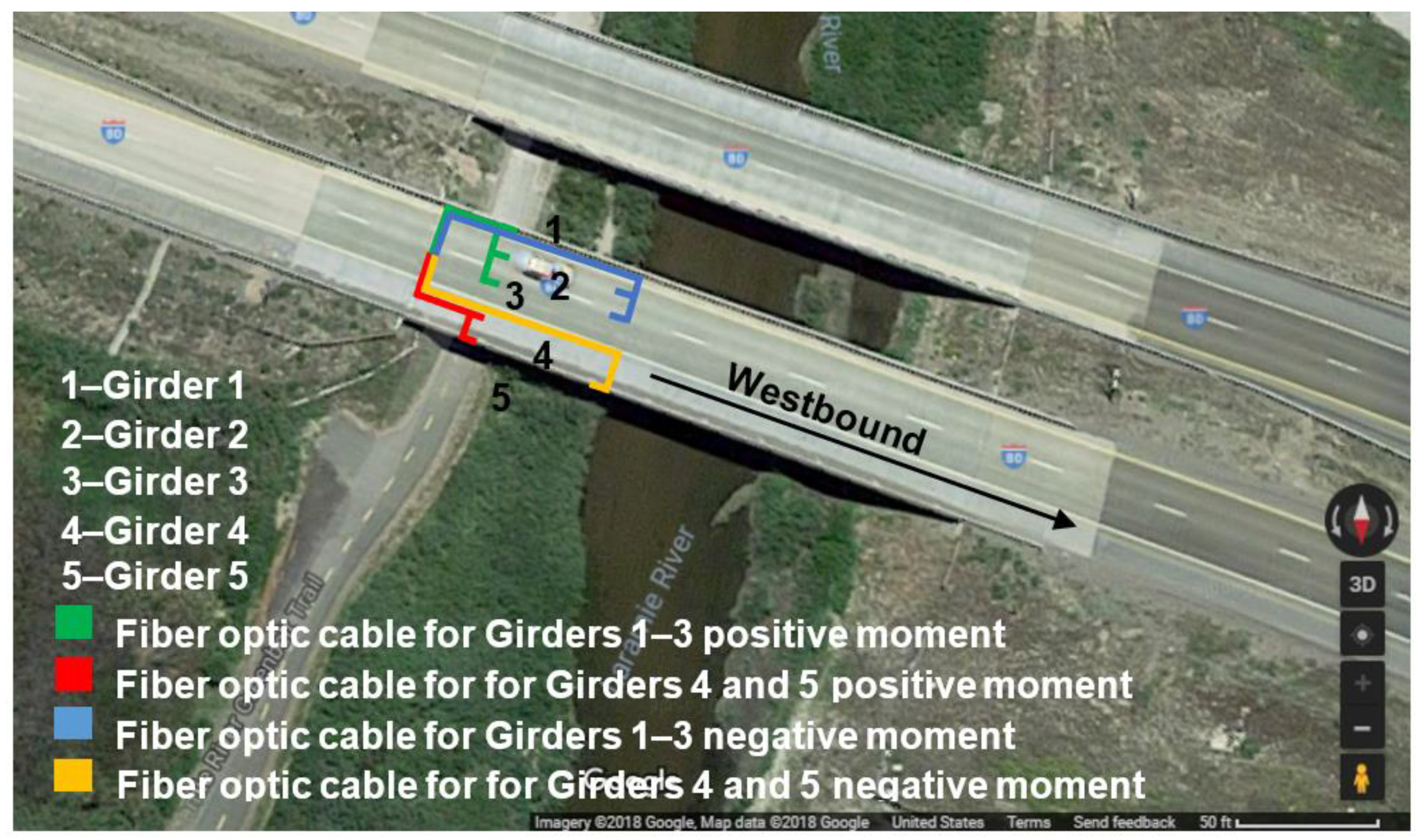
An overlay of the fiber optic cable lines and the bridge is shown in Figure 4. The river below the bridge prevented access to the inner span from the ground. Therefore, only the outer span was instrumented. Four fiber cables were installed: two cables with six sensors multiplexed and secured to Girders 1–3 and two cables with four sensors multiplexed and secured to Girders 4 and 5. It was decided to have two sensors per girder. The sensor excitation hardware used in this study can accommodate up to 25 sensors per cable.
The fiber optic sensors were mounted at both positive and negative moment locations. The critical positive moment location for the outer span was determined using a line girder analysis. For a single truck loading condition, it was located at 40% of the span length, measured from the abutment. The critical negative moment was at the pier. For the web-and-flange configuration, one sensor was installed on the bottom surface of the bottom flange, and one sensor was installed 508 mm (20 in.) above the bottom surface of the bottom flange. The sensors at the negative moment location were horizontally offset 1.52 m (5 ft) from the pier to minimize the influence of the support reaction on the measured strain [35]. For this bridge, the fiber optic sensors were mounted by applying a two-part epoxy, a resin and a curing agent, mixed in a ratio of 1:1, on the ends of the sensor. Before mounting the sensors, the surface of the girder was prepared by using a grinder. The fiber optic cables were tightly routed to the cross frames and to the girders.
The fiber optic sensors used in this study were os3120 optical strain gages manufactured by MicronOptics. The fiber optic sensor had a 22-mm gage length with fiber Bragg gratings that was protected by a stainless-steel case. The steel case can also be used to mount the sensor to a host material (i.e., the girder). A small dimple was at both ends of the sensor to accommodate the epoxy. The range of strain that the sensor could capture was ±2500 με. It could operate between −40 and 120 degrees Celsius. A fiberglass braid covered the grating region and extended 1 m from each side of the sensor. The cladding of the os3120 was made of polyamide that enveloped the silica fiber. The central wavelengths of the sensors used in the project varied from 1536 to 1560 nm in a 4 nm interval. The intervals were selected so that the sensors could be multiplexed in the same line. The fiber optic sensors were connected to fiber optic cables using arc fusion splicing.
The fiber optic sensor excitation hardware consisted of a four-channel FS 2200XT BraggMeter interrogator manufactured by FiberSensing. The interrogator had a rugged lid that offered protection to the four E2000 ports for the fiber optic cables. The interrogator could operate within a −20 to 60-degree Celsius range. The laser in the interrogator had an optical output power of −3 dBm and bandwidth of <500 MHz. To power the interrogator, it required 11–36 VDC of voltage and had a nominal consumption of 20 W and a standby consumption of 1 W. The central wavelength of each sensor was recommended by the manufacturer to be within 1500 and 1600 nm.
3.3. Strain Transducer Sensor System
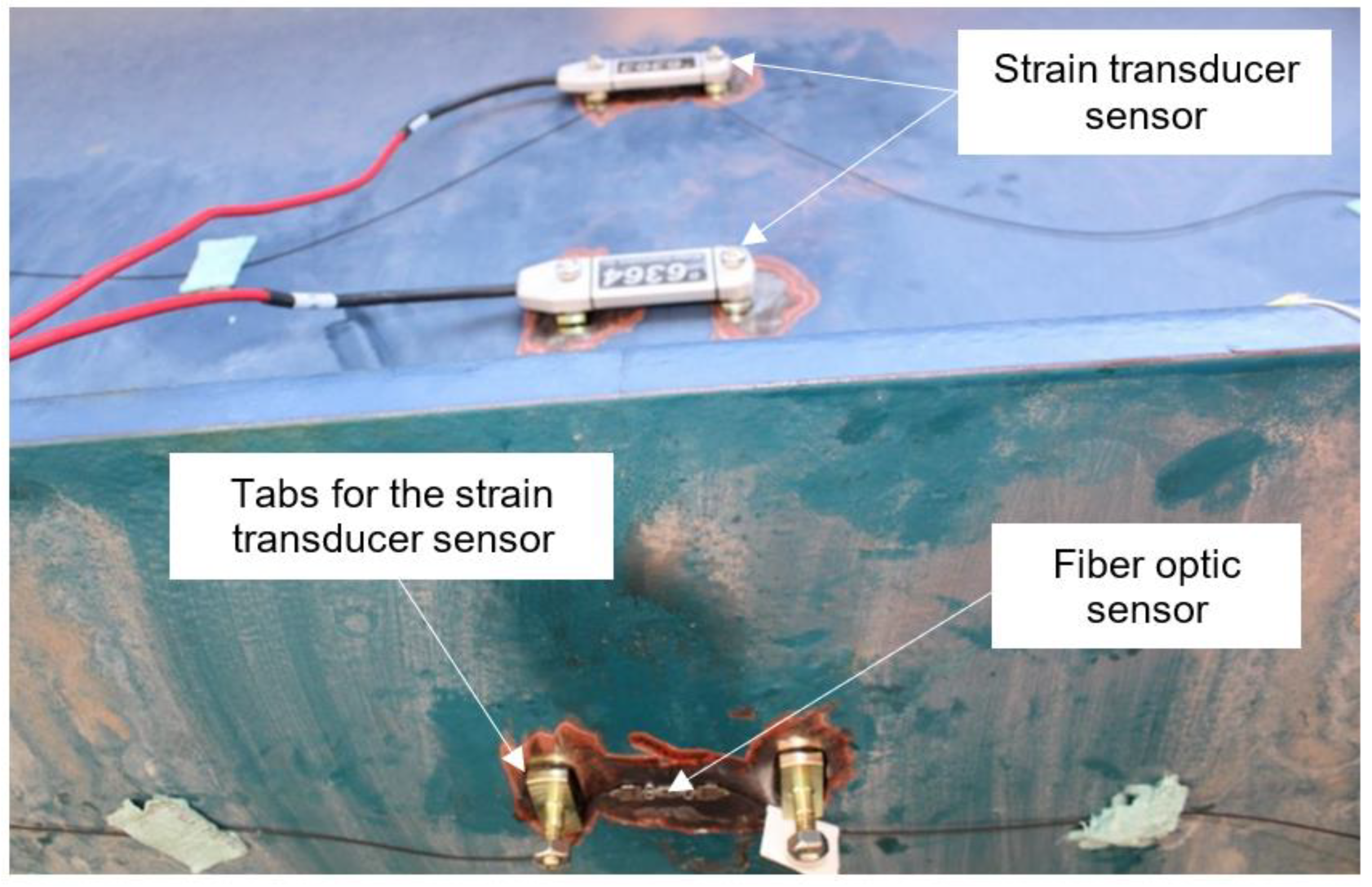
Conventional strain transducer sensors were mounted parallel to the fiber optic sensors to validate the fiber optic system. The strain transducer sensor was a ST350 ruggedized electrical transducer manufactured by Bridge Diagnostics, Inc. The ST350 sensor had a Wheatstone Bridge circuit that consisted of two chains mounted in parallel with two 350 Ω foil gages placed in series. The sensor was protected by a fully sealed and waterproof case and attached to the girders using temporary mounting tabs. The tabs were glued so that the midpoint of the sensor was aligned over the midpoint of the fiber optic sensor.
The position of the conventional sensors for a typical location is shown in Figure 5. One additional strain transducer sensor was mounted on the web (e.g., the sensor in the center of Figure 5). The strain transducer sensors were connected to a STS4-4 data acquisition box. Each STS4-4 box had four nodes. The acquisition box emitted a signal to the STS4 base station system that received and transmitted the information wirelessly to a computer.
3.4. Results
A field test was conducted in accordance with the AASHTO Manual of Bridge Evaluation [36]. In the test, ambient traffic was temporarily prevented and a single vehicle (with a weight that was calibrated to be within the linear elastic regime of the structure) was driven across the bridge at crawl speed in successive runs. Two-vehicle and three-vehicle loading cases were simulated by superimposing the results from the individual runs. The transverse position of the vehicle shifted for each run so that the maximum response of each girder was captured. In the first run, the vehicle right front wheel center was offset 0.91 m (3 ft) from the right curb. In successive runs, the wheel center was offset 0.61 m (2 ft) to the left of the previous position. A total of fifteen runs were conducted. For each run, the strain history (the variation of strain as a function of time) was recorded for both the fiber optic and the strain transducer sensors.
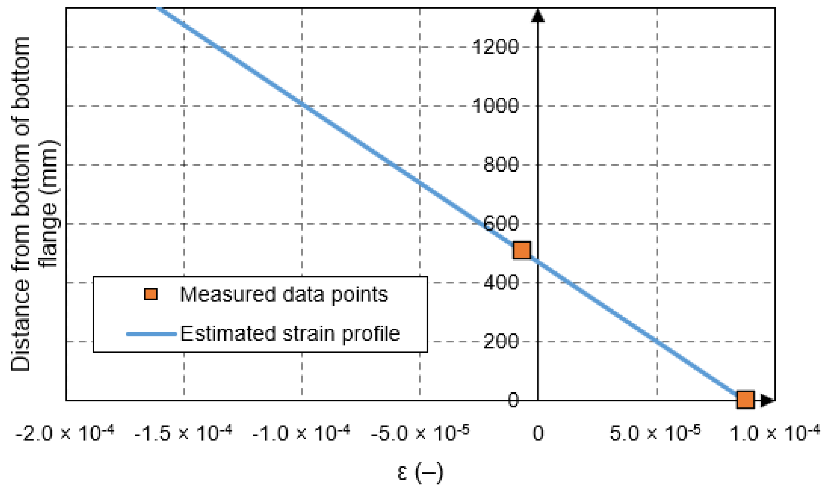
The strain profile of each girder was determined by identifying the time that the maximum peak strain occurred. The corresponding measured strains were used to calculate the internal stresses and forces in each girder. The process for postprocessing of strain data is described in [37]. During this process, it was observed that the computed neutral axis based on the sensor data was lower than the non-composite neutral axis for sensors located on the web at the same location as a transverse stiffener. This was observed even for data that corresponded to the time when the vehicle was immediately above the girder. For example, Figure 6 shows a representative strain profile at the transverse stiffener location. The figure shows that the computed neutral axis was below the fiber optic sensor that was mounted on the web 508 mm (20 in.) above the bottom surface of the bottom flange, whereas the non-composite neutral axis calculated based on the properties in Table 1 was located at 667 mm (26.3 in.) above the bottom flange. The lower location of the neutral axis at the stiffener matched that observed in [38]. As a result, the data from sensors mounted on the web at the stiffener locations were not used. To compensate for the loss of the strain data on the web at stiffener locations, the neutral axis was computed based on a full composite action between the girder and the bridge deck. This approach was considered reasonable because the loading was within the linear elastic region, and prior studies indicated that in the elastic range the bond and friction between deck and girders was maintained [39]. The implications of this approach are discussed in [40].
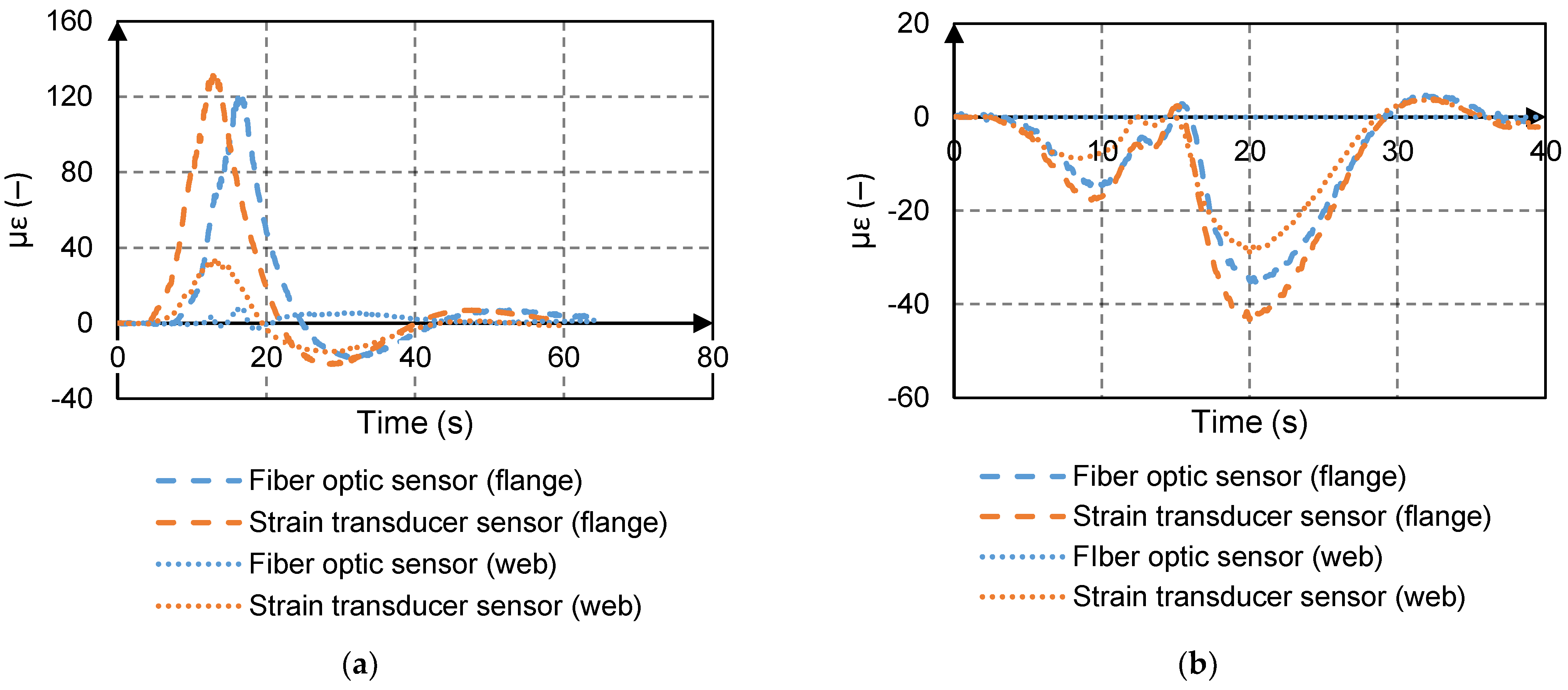
In comparison to the strain transducer sensor data, the strain histories obtained by the fiber optics system matched for girders close to the load point. The average difference for all the available sensor data for the bottom flange of the steel girders in comparison to the strain transducer data was 7%. Figure 7 shows a comparison of the fiber optic and strain transducers’ strain histories for a representative girder and run. The fiber optic sensors measured a slightly smaller strain compared to the strain transducer sensors (approximately 13 µε and 8 µε at the positive and negative moment locations, respectively). The difference between the data was consistent with results obtained in laboratory experiments [34]. Aside from aleatoric sources, the difference was attributed to two factors: first, the gage factor depends on the temperature and the thermal expansion coefficient of the host material, but the actual condition of the host material (steel) was not assessed; second, there was a lag between the fiber optic sensor response and the strain transducer sensor response (e.g., at the positive moment location).
The fiber optic data were significantly affected by the adhesive mount at some locations. For instance, as shown in Figure 7, the strain measured by the fiber optic sensor on the web was unreasonably low at the positive moment location. The lower strain reading was attributed to the integrity of the adhesive mount. Although the epoxy worked relatively well under laboratory environment, it was less effective in the field. After the field tests, the fiber optic sensors were removed, and it was observed that some of the sensors were poorly attached to the host material. The poor attachment was likely due to the uneven steel surface and possibly improper mixture of the two parts of the epoxy.
At other locations, the fiber optic signal was lost, for example, as shown in Figure 7 at the negative moment location. Loss of signal was due to damaged cables and the geometry of the cables. The damage occurred either when cables were transported to the field or during installation. Loss of signal due to geometry (routing of cables) occurred where the cables transitioned from one structural element to another (e.g., from the flange to the web or from one girder to another girder through the cross frames) with a tight bending radius.
3.5. Discussion
A disadvantage of the web-and-flange array configuration was that it required the fiber optic lines to be highly multiplexed. The results from this bridge indicated that although fiber optic lines can be multiplexed, signal loss is inevitable. In addition to the array configuration, the results showed that prior to the splicing, the fiber optic lines were also sensitive to the mounting procedure. Tight bends in the cable at flange-web transitions and transitions between flange and cross frame caused signal loss. The curing conditions required for the epoxy were difficult to ensure under field conditions, and this caused debonding of the sensors to the host material and, consequently, compromised data. As a result, a flange-only-array configuration and mechanical mounting of the sensors may be desirable to avoid signal loss and to maintain the integrity of the data. These aspects of the fiber optic system were considered in the development of the flange-only array configuration that is presented in the next section.
4. Flange-Only Array Configuration
4.1. Bridge Description
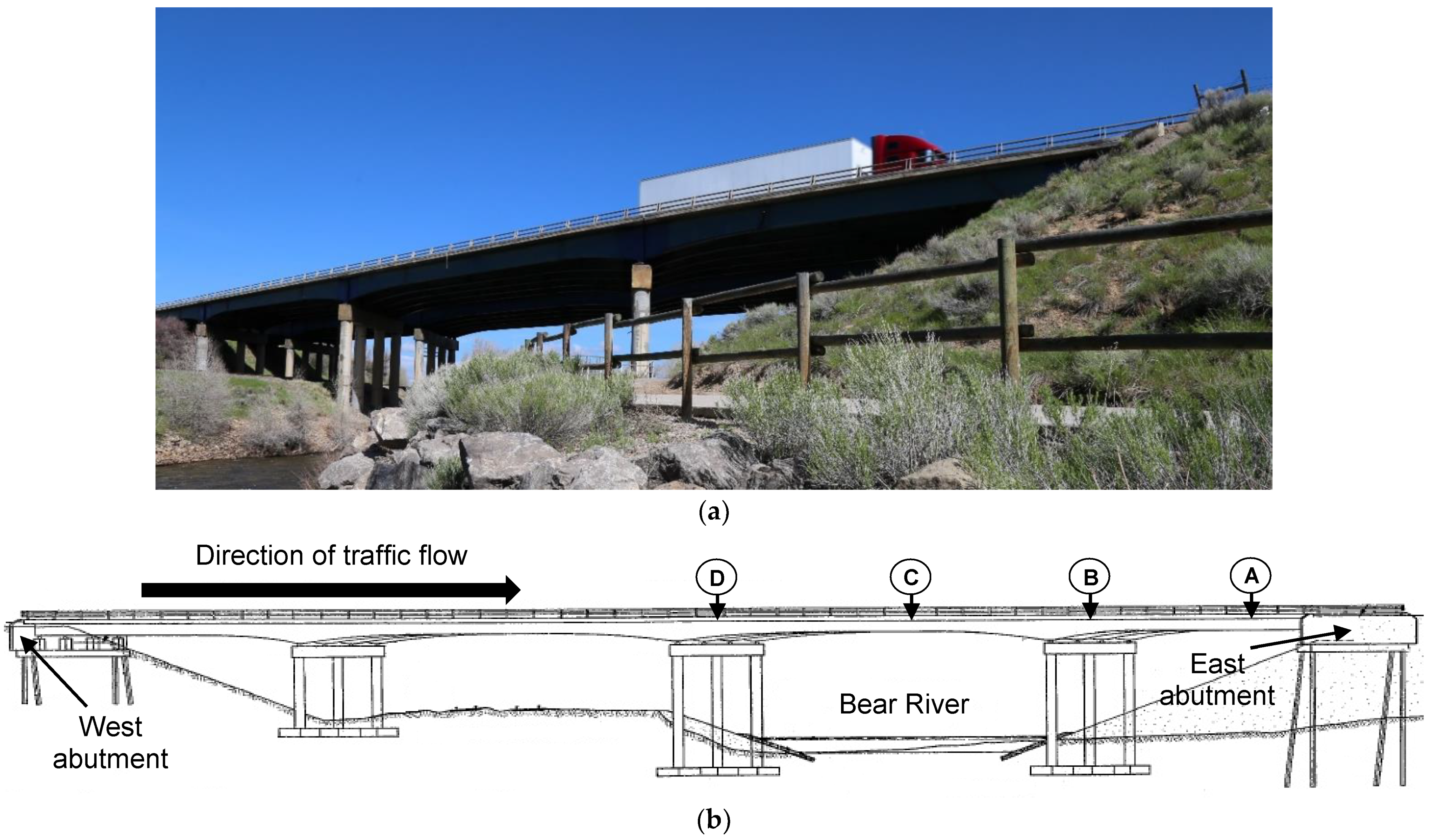
The flange-only-array configuration was installed on the eastbound bridge on Interstate 80 over the Bear River in Evanston, Wyoming, USA. The bridge is shown in Figure 8. This bridge was selected for the study, because it had the most stringent weight restrictions of non-slab bridges along Interstate 80. The bridge is a symmetric continuous bridge with four spans. The outer span is 25.6 m (84 ft) and inner span is 36.6 m (120 ft). The bridge is horizontally skewed 47 degrees. The bridge deck is supported by five I-shape steel plate girders. Similar to the Laramie River bridge, the Bear River bridge was originally constructed with four girders (Girders 1–4) and later widened with a fifth girder (Girders 5). The original girders were designed to act non-compositely with the deck. Girder 5 has shear studs on the top flange.
The clear roadway width is approximately 12.2 m (40 ft) with curbs and barrier rails on the western side and just curbs on the eastern side. The spacing between girders is 2.74 m (9 ft). The deck thickness is 191 mm (7.5 in.) with a future wearing surface of 38.1 mm (1.5 in.) above it. At the eastern pier the girders are supported by a fixed bearing. The girders are supported by expansion bearings at the other abutment and at the interior piers. At the piers, the girders are spliced and the depth of the girders increases. The web and flange of the girders are thicker than the girders on the bridge span.
The dimensions of the girders at selected locations shown in Figure 8 are given in Table 2. All girders were specified to be 248 MPa (36 ksi) A36 structural steel. The concrete used for the original and added deck was specified to have a nominal compressive strength equal to 22.4 MPa (3250 psi) and 27.6 MPa (4000 psi), respectively. The longitudinal reinforcement is Grade 60, and the stirrups are Grade 40. Cross bracings are present on each span normal to the girders. Expansion joints are located at the piers and at the abutments.
4.2. Fiber Optic System
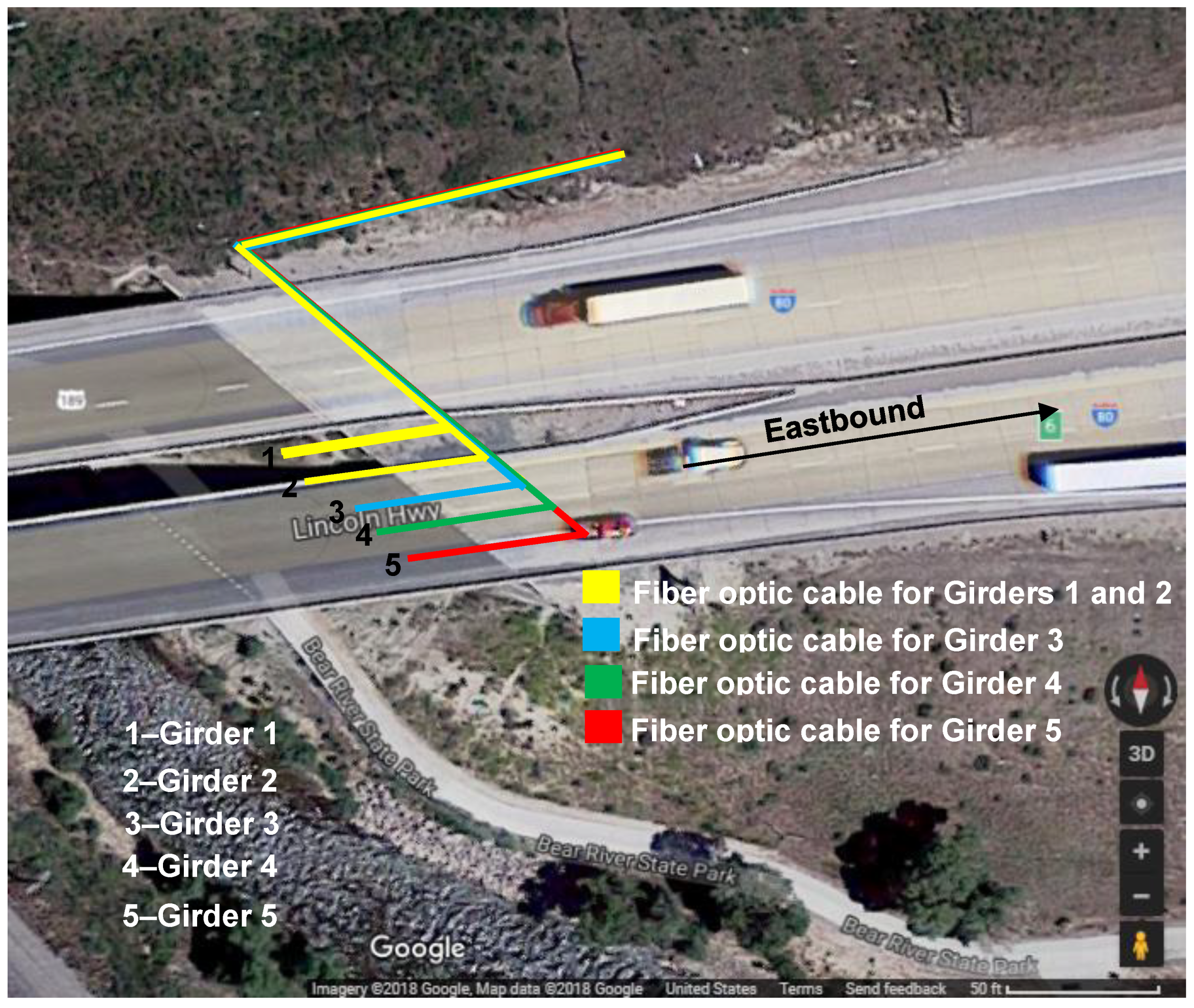
An overlay of the fiber optic cable lines and the bridge is shown in Figure 9. Four fiber cables were installed, one cable with two strain sensors multiplexed and secured to each girder. The strain sensors were used in tandem with unrestrained fiber optic temperature compensation sensors. As was the case with the first bridge, for the second bridge the inner span was not accessible from the ground due to the river. Therefore, only the outer span was instrumented. The critical positive moment location for the outer span for a single truck loading condition was determined to be located 7.32 m (24 ft) from the east abutment.
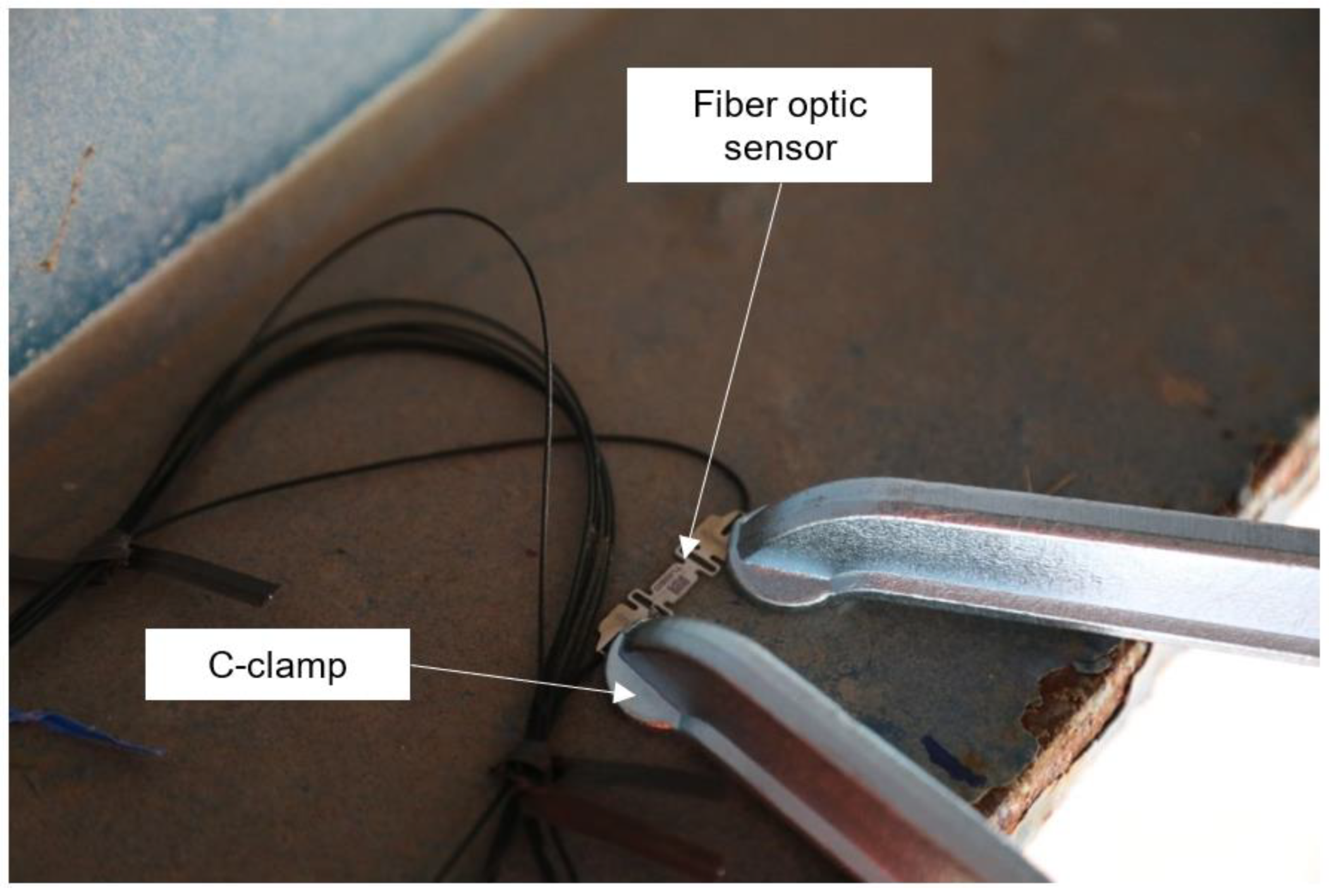
Prior to installing the fiber optic system, the elastic neutral axis of the girders was determined by installing strain transducer sensors, conducting a diagnostic field test, and then removing the sensors. The fiber optic system was afterwards installed on each girder at the positive moment location. The fiber optic strain sensor was mounted to the top surface of the bottom flange using a C-clamp. Two C-clamps were used for each sensor, as shown in Figure 10. The C-clamps were attached to the end of the sensor casing to avoid pinching the fiber optic line.
The interrogator, a compact computer, a cellular modem, and a remote power switch were housed onsite in a cabinet near the bridge. The fiber optic cables were loosely routed to the cross frames and to the girders. The fiber optic cables exited the north side of the bridge along the ground near the guardrail to the cabinet.
The structural health monitoring system was then tested using a calibrated vehicle. The calibrated vehicle was similar to the one used in the field tests. However, unlike the field tests, the bridge was not closed to traffic and the calibrated vehicle crossed the bridge in three alternating westbound and eastbound runs, for a total of six runs. The vehicle was also driven at high speed, 105 km/h (65 mph) to 113 km/h (70 mph), instead of crawl speed as was performed in the field tests.
4.3. Results
The live load contribution of the bridge load carrying capacity, , at the positive moment location for a single truck was calculated as
where is the analytical moment due to a standardized design truck, is the analytical maximum moment due to the calibrated truck used in the field test, and is the live load non-composite moment in the girder. For this bridge, the design load was equal to the HS20 vehicle load, because the Load Factor Design (LFD) method [41] was used in the original design. Based on a line girder analysis, was 1300 kN-m, and was 891 kN-m. Based on the strain profile from the field test, was equal to 164 kN-m for the test run that maximized the response of Girder 3.Thus, for the field test was 240 kN-m.
The results from the calibrated vehicle driven at high speed (“SHM test”) are summarized with the field test results in Table 3. The strain was 81.3 µε in the bottom flange. To determine the strain profile, the degree of composite action in the SHM test was based on the degree of composite action (59% of full composite action) determined in the field test. Therefore, for the SHM test was 168 kN-m and was 250 kN-m. The values of and were essentially constant (2% different due to the weight).
The results demonstrated that the strains captured by the fiber optic system and the conventional system agreed relatively well. The strains were essentially the same at Girder 3 (the girder with the peak strain) directly under the vehicle load. The largest difference approached the noise of the signal at Girders 1 and 4 (the girders with small strain) located away from the vehicle load. The difference in the strains reflects several factors: the distance between the vehicle load and the sensors [42], the lag in sensor response (as was observed in the bridge with the web-and-flange array), and the difference in the vehicle weights and speeds.
4.4. Discussion
Compared to the web-and-flange array, the flange-only array required fewer sensors. Since the array was multiplexed fewer times, signal loss was minimized, and sensor detection was encouraged. Routing of fiber optic cables could also be simplified to mitigate signal loss.
Unlike the adhered sensors in the web-and-flange array, all sensors in the mechanically mounted flange-only array remained attached to the girder. Thus, in this study no data were lost using the flange-only array configuration. However, the flange-only configuration required the neutral axis of the girders to be determined beforehand. This could be accomplished either through field tests (as in this study) or through simulation (i.e., finite element modeling).
For this bridge, the girders in the outer span could be partially accessed by the Bear River State Park trail (the trail is visible in Figure 9). Consequently, the fiber optic cables were dislodged and vandalized a few months after installation. To avoid this in a future placement, a conduit could be trenched from the equipment cabinet to the bridge abutment, and the fiber optic cable exiting the conduit at the steel girder could be protected using a modified butyl rubber tape. Alternatively, for this bridge the inner span could be used if a snooper truck was available so that access to sensors was provided from above.
5. Conclusions
A structural health monitoring system was developed using fiber optic sensors based on fiber Bragg gratings. The system was deployed on two highway bridges. For the first bridge, fiber optic sensors were glued with epoxy resin to the girder webs and flanges in a web-and-flange array that permitted determination of the elastic neutral axis of the girder. To validate the system, strain transducer sensors were installed parallel to the fiber optic sensors, and a field test was conducted. For the second bridge, a flange-only array of fiber optic sensors was used. The sensors were mounted to the girder bottom flange using C-clamps. The elastic neutral axis of the girders was determined by conducting a field test with conventional strain transducer sensors. After the field test, the conventional sensors were removed, and a fiber optic system was later installed.
The following are the primary findings of the study:
- Measured strain data from fiber optic sensors were reasonably close to the data measured using strain transducer sensors.
- Sensors in a web-and-flange array were prone to signal loss because the cables were highly multiplexed and tightly routed along the girder and cross frames. In contrast, sensors in the flange-only array better maintained signal integrity compared to the web-and-flange array because the configuration involved fewer multiplexed cables and had loosely routed cables.
- Adhesive mounting of fiber optic strain sensors was not reliable because the conditions for proper curing, which were easily created in the laboratory, were difficult to ensure in the field. For the two bridges examined in this study, mechanical mounting of fiber optic strain sensors was more effective than the adhered mounting of sensors.
Based on these findings, we recommend using the minimum number of sensors required to adequately monitor the structural response of interest when deploying a fiber optic structural health monitoring system. Moreover, we recommend using a large radius of curvature when routing fiber optic cables. Using adhesives to mount sensors is not recommended for long-term monitoring. Mechanical mounts are suggested for measuring strains in unstiffened elements of the girder cross section (i.e., the flange). For a mechanical mount application to measure girder strains, it is necessary to determine the elastic neutral axis of the girder using a field test or a finite element analysis. Regardless of the configuration or the type of mount, sensors that are left in place for long period of time need to be protected from vandalism and wildlife.
The results also suggest that fiber optic sensor-based structural monitoring systems may be best suited in a hybrid approach where, for short-term monitoring, a diagnostic field test with conventional sensors is used to determine the neutral axis of each girder and the baseline bridge response, and the fiber optic sensors are used to periodically monitor bridge performance. For long-term monitoring, the short-term data can be stitched together to form a long-term record.
The structural health monitoring system proposed in this paper takes advantage of the rapid installation made possible by modern fiber optic and strain-transducer sensors. It avoids the difficulty inherent in creating a permanent installation, and when needed, facilitates the repair and maintenance of sensors compared to embedded sensors. Since the proposed system is redeployable, the proposed scheme also allows the interrogator and the sensors, which are high-cost components of the system, to be reused multiple times and at multiple highway bridges.
Two key features of a deployable structural health monitoring system that were not fully addressed in this study are (1) methods for remote data collection, and (2) postprocessing of data. Since many bridges are isolated or in locations with harsh environments, onsite data collection can be inconvenient or impractical. In this study, a compact computer was located at the bridge and used to control the interrogator, record data (function as a data logger), filter data, and store data for transmission, and execute data transmission over a cellular network. However, best practices for data collection have yet to be determined. Additional research is needed to determine effective methods for postprocessing of data because structural health monitoring systems can produce very large datasets. Efficiently extracting data then becomes of paramount importance. In this study, data corresponding to the field tests were manually extracted, but it would be desirable to develop an efficient approach to data mining. In sum, a critical gap in structural health monitoring systems that needs to be closed is the development of a complete Internet of Things (IoT) platform that addresses both data collection and data analysis.
Author Contributions
Conceptualization, R.L. and J.J.; methodology, R.L and J.J.; validation, R.L. and J.J.; formal analysis, R.L.; resources, J.J.; data curation, J.J.; writing—original draft preparation, J.J.; writing—review and editing, R.L. and J.J.; supervision, J.J.; project administration, J.J.; funding acquisition, J.J. All authors have read and agreed to the published version of the manuscript.
Funding
This research was funded by the Wyoming Department of Transportation (WYDOT) and the Federal Highway Administration of the USA, grant number RS06216 and the State of Wyoming through the Department of Civil and Architectural Engineering.
Institutional Review Board Statement
Not applicable.
Informed Consent Statement
Not applicable.
Data Availability Statement
The measured strain data, analytical models, and spreadsheets generated or used during the study are available from the corresponding author by reasonable request.
Acknowledgments
The authors appreciate the support of WYDOT personnel in installing systems and conducting the field tests. The views expressed in this paper are those of the authors and do not necessarily reflect the views of those acknowledged.
Conflicts of Interest
The authors declare no conflict of interest. The funders had no role in the design of the study; in the collection, analyses, or interpretation of data; in the writing of the manuscript, or in the decision to publish the results.
References
- American Society of Civil Engineers (ASCE). 2021 Report Card for America’s Infrastructure; ASCE: Reston, VA, USA, 2021. [Google Scholar]
- Bell, E.S.; Lefebvre, P.J.; Sanayei, M.; Brenner, B.; Sipple, J.D.; Peddle, J. Objective load rating of steel-girder bridge using structural modeling and health monitoring. J. Struct. Eng. 2013, 139, 1771–1779. [Google Scholar] [CrossRef]
- Collins, J.; Mullins, G.; Lewis, C.; Winters, D. State of the Practice and Art for Structural Health Monitoring of Bridge Substructures; Report No. FHWA-HRT-09-040; Turner-Fairbank Highway Research Center, United States Department of Transportation, Federal Highway Administration: McLean, VA, USA, 2014. [Google Scholar]
- Moyo, P.; Brownjohn, J.M.W.; Suresh, R.; Tjin, S.C. Development of fiber Bragg grating sensors for monitoring civil infrastructure. Eng. Struct. 2005, 27, 1828–1834. [Google Scholar] [CrossRef]
- Vardanega, P.J.; Webb, G.T.; Fidler, P.R.A.; Middleton, C.R. Chapter 29—Bridge monitoring. In Innovative Bridge Design Handbook Construction, Rehabilitation and Maintenance; Pipinato, A., Ed.; Butterworth-Heinemann: Oxford, UK, 2016; pp. 759–775. ISBN 9780128000588. [Google Scholar]
- Modares, M.; Waksmanski, N. Overview of structural health monitoring for steel bridges. Pract. Period. Struct. Des. Constr. 2013, 18, 187–191. [Google Scholar] [CrossRef]
- Santarsiero, G.; Masi, A.; Picciano, V.; Digrisolo, A. The Italian guidelines on risk classification and management of bridges: Applications and remarks on large scale risk assessments. Infrastructures 2021, 6, 111. [Google Scholar] [CrossRef]
- Maes, K.; Van Meerbeeck, L.; Reynders, E.P.B.; Lombaert, G. Validation of vibration-based structural health monitoring on retrofitted railway bridge KW51. Mech. Syst. Signal Process. 2022, 165, 108380. [Google Scholar] [CrossRef]
- Sony, S.; Gamage, S.; Sadhu, A.; Samarabandu, J. Multiclass damage identification in a full-scale bridge using optimally tuned one-dimensional convolutional neural network. J. Comput. Civ. Eng. 2022, 36, 04021035. [Google Scholar] [CrossRef]
- Li, X.; Xiao, Y.; Guo, H.; Zhang, J. A BIM based approach for structural health monitoring of bridges. KSCE J. Civ. Eng. 2022, 26, 155–165. [Google Scholar] [CrossRef]
- Catbas, F.N. Structural health monitoring: Applications and data analysis. In Structural Health Monitoring of Civil Infrastructure Systems; Karbhari, V.M., Ansari, F., Eds.; Woodhead Publishing Limited: Sawston, UK, 2009; pp. 1–39. [Google Scholar]
- Zhang, B.; Benmokrane, B.; Nicole, J.F.; Masmoudi, R. Evaluation of fibre optic sensors for structural condition monitoring. Mater. Struct. 2002, 35, 357–364. [Google Scholar] [CrossRef]
- Tennyson, R.C.; Mufti, A.A.; Rizkalla, S.; Tadros, G.; Benmokrane, B. Structural health monitoring of innovative bridges in Canada with fiber optic sensors. Smart Mater. Struct. 2001, 10, 560–573. [Google Scholar] [CrossRef]
- Kersey, A.D.; Davis, M.A.; Patrick, H.J.; LeBlanc, M.; Koo, K.P.; Askins, C.G.; Putman, M.A.; Friebele, E.J. Fiber grating sensors. J. Light. Technol. 1997, 15, 1442–1463. [Google Scholar] [CrossRef] [Green Version]
- Webb, G.T.; Vardenga, P.J.; Hoult, N.A.; Fidler, R.A.; Bennett, P.J.; Middleton, C.R. Analysis of fiber optic strain-monitoring data from a prestressed concrete bridge. J. Bridge Eng. 2017, 22, 05017002. [Google Scholar] [CrossRef] [Green Version]
- Maaskant, R.; Alavie, T.; Measures, R.M.; Tadros, G.; Rizkalla, S.H.; Guha-Thakurta, A. Fiber-optic Bragg grating sensors for bridge monitoring. Cem. Concr. Compos. 1997, 19, 21–33. [Google Scholar] [CrossRef]
- Wan, C.; Hong, W.; Liu, J.; Wu, Z.; Xu, Z.; Li, S. Bridge assessment and health monitoring with distributed long-gauge FBG sensors. Int. J. Distrib. Sens. Netw. 2013, 9, 494260. [Google Scholar] [CrossRef]
- Casas, J.R.; Cruz, P.J. Fiber optic sensors for bridge monitoring. J. Bridge Eng. 2003, 8, 362–373. [Google Scholar] [CrossRef] [Green Version]
- Regier, R.; Hoult, N.A. Distributed strain behavior of a reinforced concrete bridge: Case study. J. Bridge Eng. 2014, 19, 05014007. [Google Scholar] [CrossRef]
- Kong, X.; Ho, S.C.M.; Song, G.B.; Cai, C.S. Scour monitoring system using fiber Bragg grating sensor and water swellable polymers. J. Bridge Eng. 2017, 22, 04017029. [Google Scholar] [CrossRef]
- Jeon, J.; Lee, J.; Shin, D.; Park, H. Development of dam safety management system. Adv. Eng. Softw. 2009, 40, 554–563. [Google Scholar] [CrossRef]
- Sharma, V.B.; Singh, K.; Gupta, R.; Joshi, A.; Dubey, R.; Gupta, V.; Bharadwaj, S.; Zafar, M.I.; Bajpai, S.; Khan, M.A.; et al. Review of structural health monitoring techniques in pipeline and wind turbine industries. Appl. Syst. Innov. 2021, 4, 59. [Google Scholar] [CrossRef]
- Bossi, G.; Schenato, L.; Marcato, G. Structural health monitoring of a road tunnel intersecting a large and active landslide. Appl. Sci. 2017, 7, 1271. [Google Scholar] [CrossRef] [Green Version]
- Wu, T.; Liu, G.L.; Xing, F. Recent progress of fiber-optic sensors for the structural health monitoring of civil infrastructure. Sensors 2020, 20, 4517. [Google Scholar] [CrossRef]
- Costa, B.J.; Figueiras, J.A. Evaluation of a strain monitoring system for existing steel railway bridges. J. Constr. Steel Res. 2012, 72, 179–191. [Google Scholar] [CrossRef]
- Van der Kooi, K.; Hoult, N.A.; Le, H. Monitoring and in-service railway bridge with a distributed fiber optic strain sensing system. J. Bridge Eng. 2018, 23, 05018007. [Google Scholar] [CrossRef]
- Cocking, S.; Alexakis, H.; DeJong, M. Distributed dynamic fibre-optic strain monitoring of the behaviour of a skewed masonry arch railway bridge. J. Civ. Struct. Health Monit. 2021, 11, 989–1012. [Google Scholar] [CrossRef]
- Gebremichael, Y.M.; Li, W.; Meggit, B.T.; Boyle, W.J.; Grattan, K.T.; McKinley, B.; Boswell, L.F.; Aarnes, K.A.; Aasen, S.E.; Tynes, B.; et al. Field deployable, multiplexed Bragg grating sensor system used in an extensive highway bridge monitoring evaluation tests. IEEE Sens. J. 2005, 5, 510–519. [Google Scholar] [CrossRef]
- Doornink, J.D. Monitoring the Structural Condition of Fracture-Critical Bridges Using Fiber Optic Technology. Ph.D. Thesis, Iowa State University, Ames, IA, USA, 2006. [Google Scholar]
- Phares, B.M.; Greimann, L.; Choi, H. Integration of Bridge Damage Detection Concepts and Components Volume I: Strain-Based Damage Detection; Report No. IHRB Project TR-636; Iowa Department of Transportation: Ames, IA, USA, 2013. [Google Scholar]
- Hubbard, P.; Yust, M.; Costley, R.; Cox, B.; Menq, F.; Murphy, J.; Soga, K. Distributed Acoustic Sensing (DAS) data from the NHERI@UTexas Thumper Shaker Truck and 240 m of Fiber Along the Blackhawk Levee. In Proceedings of the NHERI@UTexas DAS Levee Imaging Workshop, DesignSafe-CI, Baton Rouge, LA, USA, 21–22 October 2021. [Google Scholar] [CrossRef]
- Maurais, D.T. Strain Transfer Behavior of Notch Embedded Fiber Bragg Gratings. Master’s Thesis, University of Wyoming, Laramie, WY, USA, 2012. [Google Scholar]
- Jung, M.A. Development of a Fiber Optic Based Load Testing System for Highway Bridges. Master’s Thesis, University of Wyoming, Laramie, WY, USA, 2015. [Google Scholar]
- Danforth, M.M. Laramie River Bridge Load-Testing Plan with Sensor Verification and RFID Feasibility of Permitted Vehicles. Master’s Thesis, University of Wyoming, Laramie, WY, USA, 2015. [Google Scholar]
- Barker, M.G. Quantifying field test behavior for rating steel girder bridges. J. Bridge Eng. 2001, 6, 254–261. [Google Scholar] [CrossRef]
- American Association of State Highway and Transportation Officials (AASHTO). Manual for Bridge Evaluation, 3rd ed.; AASHTO: Washington, DC, USA, 2018. [Google Scholar]
- Lu, R.; Judd, J.P.; Barker, M.G. Field load rating and grillage analysis method for skewed steel girder highway bridges. J. Bridge Eng. 2021, 26, 05021013. [Google Scholar] [CrossRef]
- Hendy, C.R.; Presta, F. Transverse web stiffeners and shear moment interaction for steel plate girder bridges. Struct. Eng. 2008, 86, 017. [Google Scholar]
- Yarnold, M.T.; Golecki, T.; Weidner, J. Identification of composite action through truck load testing. Front. Built Environ. 2018, 4, 74. [Google Scholar] [CrossRef]
- Lu, R.; Judd, J.P. Field testing of highway bridges enhanced by assumptions of composite action. In Proceedings of the International Conference on Advances in Technology and Computing—Advancements in Applications of Engineering and Science in Technology, Kelaniya, Sri Lanka, 18–19 December 2021. [Google Scholar]
- American Association of State Highway and Transportation Officials (AASHTO). AASHTO Standard Specifications for Highway Bridges, 17th ed.; AASHTO: Washington, DC, USA, 2002. [Google Scholar]
- Lu, R.; Judd, J.P. Field evaluation of unintended composite action between steel plate girders and concrete slab in highway bridges. Ce/Papers 2019, 3, 171–180. [Google Scholar] [CrossRef]
Figure 1.
Fiber Bragg grating sensor.

Figure 2.
Fiber optic sensor configurations: (a) web-and-flange array; (b) flange-only array.

Figure 3.
Bridge with web-and-flange array: (a) westbound structure; (b) elevation drawing.

Figure 4.
Fiber optic system for the bridge with the web-and-flange array.

Figure 5.
Location of the fiber optic and strain transducer sensors on a girder.

Figure 6.
Strain profile of girder at transverse stiffener location.

Figure 7.
Strain histories: (a) positive moment location; (b) negative moment location.

Figure 8.
Bridge with flange-only array: (a) eastbound structure; (b) elevation drawing.

Figure 9.
Fiber optic system for the bridge with the flange-only array.

Figure 10.
Fiber optic sensor mounted to bottom flange using C-clamps.


Table 1.
Nominal section dimensions, mm (in.), at selected locations of bridge with web-and-flange sensor array.
Table 1.
Nominal section dimensions, mm (in.), at selected locations of bridge with web-and-flange sensor array.
| Location | Top Flange Width | Top Flange Thickness | Web Height | Web Thickness | |
|---|---|---|---|---|---|
| A | Girders 1–4 | 305 (12) | 19.1 (0.75) | 1300 (51) | 9.53 (0.38) |
| Girder 5 | 305 (12) | 19.1 (0.75) | 1300 (51) | 11.1 (0.44) | |
| B | Girders 1–4 | 305 (12) | 25.4 (1) | 1300 (51) | 1300 (51) |
| Girder 5 | 305 (12) | 19.1 (0.75) | 1300 (51) | 11.1 (0.44) | |
Table 2.
Nominal section dimensions, mm (in.), at selected locations of bridge with flange-only array.
Table 2.
Nominal section dimensions, mm (in.), at selected locations of bridge with flange-only array.
| Location | Top Flange Width | Top Flange Thickness | Web Height | Web Thickness | Bottom Flange Width | Bottom Flange Thickness | |
|---|---|---|---|---|---|---|---|
| A | Girders 1–4 | 330 (13) | 25.4 (1) | 1450 (57) | 7.87 (0.31) | 330 (13) | 25.4 (1) |
| Girder 5 | 305 (12) | 15.9 (0.63) | 1370 (54) | 14.3 (0.56) | 305 (12) | 25.4 (1) | |
| B | Girders 1–4 | 330 (13) | 25.4 (1) | 1450–2210 (57–87) | 7.87 (0.31) | 330 (13) | 25.4 (1) |
| Girder 5 | 305 (12) | 25.4 (1) | 1370–2130 (54–84) | 14.3 (0.56) | 305 (12) | 25.4 (1) | |
| C | Girders 1–4 | 330 (13) | 28.7 (1.13) | 1450 (57) | 7.87 (0.31) | 330 (13) | 28.7 (1.13) |
| Girder 5 | 305 (12) | 15.9 (0.63) | 1370 (54) | 14.3 (0.56) | 305 (12) | 25.4 (1) | |
| D | Girders 1–4 | 330 (13) | 31.8 (1.25) | 1450–2240 (57–88) | 7.87 (0.31) | 330 (13) | 31.8 (1.25) |
| Girder 5 | 305 (12) | 25.4 (1) | 1370–2130 (54–84) | 14.3 (0.56) | 305 (12) | 25.4 (1) | |
Table 3.
Measured strain (µε).
| Test | Girder 1 | Girder 2 | Girder 3 | Girder 4 | Girder 5 |
|---|---|---|---|---|---|
| SHM | 14.6 | 37.3 | 81.3 | 43.1 | 16.3 |
| Diagnostic | 12.3 | 33.0 | 79.8 | 49.5 | 14.4 |
Publisher’s Note: MDPI stays neutral with regard to jurisdictional claims in published maps and institutional affiliations. |
© 2022 by the authors. Licensee MDPI, Basel, Switzerland. This article is an open access article distributed under the terms and conditions of the Creative Commons Attribution (CC BY) license (https://creativecommons.org/licenses/by/4.0/).
Share and Cite
MDPI and ACS Style
Lu, R.; Judd, J. Field-Deployable Fiber Optic Sensor System for Structural Health Monitoring of Steel Girder Highway Bridges. Infrastructures 2022, 7, 16. https://doi.org/10.3390/infrastructures7020016
AMA Style
Lu R, Judd J. Field-Deployable Fiber Optic Sensor System for Structural Health Monitoring of Steel Girder Highway Bridges. Infrastructures. 2022; 7(2):16. https://doi.org/10.3390/infrastructures7020016
Chicago/Turabian StyleLu, Renxiang, and Johnn Judd. 2022. "Field-Deployable Fiber Optic Sensor System for Structural Health Monitoring of Steel Girder Highway Bridges" Infrastructures 7, no. 2: 16. https://doi.org/10.3390/infrastructures7020016