Comparative Assessment of Criticality Indices Extracted from Acoustic and Electrical Signals Detected in Marble Specimens

Abstract

The quantitative determination of the current load carrying capability of already loaded structural elements and the possibility to detect proper indices that could be considered as signals for timely warning that the load carrying capacity is exhausted is the subject of this study. More specifically, it aims to explore the possibility of detecting signals that can be considered as indices warning about upcoming fracture and then to compare quantitatively such signals provided by different techniques. The novelty of the present study lies exactly in this quantitative comparison of the pre-failure signals provided by various sensing techniques and various methods of analysis of the experimental data. To achieve this target, advantage is taken of data concerning the acoustic and electrical activities produced while marble specimens are subjected to mechanical loading. The respective signals are detected and recorded by means of the acoustic emissions technique and that of the pressure stimulated currents. The signals detected by the acoustic emissions technique are analyzed in terms of three formulations, i.e., the b-value, the F-function and the parameters variance κ₁, entropy S and entropy under time reversal S_ according to the natural time analysis. The signals detected by the pressure stimulated currents technique are analyzed by means of the intensity of the electric current recorded. The study indicates that all quantities considered provide promising pre-failure indicators. Furthermore, when the specimen is subjected to near-to-failure load levels, the temporal evolution of three of the quantities studied (b-value, F-function, pressure stimulated currents) is governed by a specific power law. The onset of validity of this law designates some differentiation of the damage mechanisms activated. Quantitative differences are observed between the time instants at which this power law starts dictating the evolution of the above parameters, indicating the imperative need for further investigation, despite the quite encouraging results of the present study.

1. Introduction

The mechanical response of structures at load levels approaching those causing failure, as well as their remaining load-carrying capacity, is of crucial importance for structural engineers, independently of whether the structures are intact or already pre- cracked. In this direction, intensive technological research is carried out worldwide aiming to develop sophisticated structural health monitoring (SHM) tools which can record even the slightest deviations from the expected response of the monitored structure, warning, thus, about upcoming local or global failure.

Nowadays, the most widely used SHM tools are based on the detection and recording of either acoustic [1,2,3] or electric [4,5,6,7] signals, emitted while structural members are loaded by mechanical stimuli. The proper interpretation of the data acquired by these sensing techniques, in the direction of revealing hidden pre-failure indicators, is among the challenges of the current scientific research [8,9]. Various approaches have been proposed to analyze the experimental data, such as the b-value analysis [10,11], models based on wavelets [12,13] and natural time (NT) [14,15], analyses based on non-extensive statistical physics (NESP) [16,17], power-law models [18,19] etc.

In this study, a comparative consideration of the pre-failure indices provided by some of these approaches is described. A short section with some theoretical preliminaries concerning the physical background of the sensing techniques, based on acoustic and electric emissions, follows. Then, the parameters used to analyze the experimental data are briefly described, including the b-values, the F-function, the natural time parameters variance κ₁, entropy S and entropy under time reversal S_ and, finally, the pressure stimulated currents (PSCs). Then, acoustic and electric data, obtained from two experimental protocols with specimens made of Dionysos marble, are analyzed in terms of the aforementioned four parameters, in an attempt to comparatively discuss their time evolution as well as the time instants of appearance of the pre-failure indices provided by each one. A flow chart of the structure of the study is shown in Figure 1.

According to the above flow chart, the experimental protocols are carried out, paying special attention to accurately determining the time instant of macroscopic fracture, t_f. The latter is achieved by taking advantage of the hits recorded by the acoustic sensors, recalling that at the instant of macroscopic fracture a signal of amplitude equal to 99 dB is usually recorded (obviously the compatibility of this value with the respective records of the mechanical parameters is sine qua non for the final decision concerning the exact fracture instant). Then the raw acoustic data (time instant of occurrence of the acoustic signals, their amplitude and their energy) are properly analyzed in order to determine the parameters required by the natural time or the Ib-value analyses, as well as that of the F-function. Simultaneously the data provided by the electric sensors are analyzed in terms of the intensity of the PSCs recorded. Then, the temporal evolution of the parameters considered is explored, in order to detect the changes that could be assumed as designating the entrance of the system into its critical stage, namely the stage of impending macroscopic fracture. Finally, the pre-failure signals determined as above are mutually compared quantitatively. It is exactly this quantitative consideration of the pre-failure indices provided by various sensing techniques and various methods of analysis of the experimental data, which are based on definitely different natural principles, that highlights the novelty of the present study.

The study reveals that all four parameters provide signs that could be potentially considered as proper pre-failure indicators. In addition, during the very last loading steps the temporal evolution of the b-value, the F-function and that of the weak electric currents obey a power law. It is assumed that the onset of validity of this law designates activation of different damage mechanisms, i.e., those that eventually will lead to macroscopic fracture. The time instants, at which the above parameters provide their pre-failure indicator, do not coincide with each other. However, they are in relatively satisfactory mutual agreement, suggesting that the underlying damage mechanisms, activated while the specimen tends to exhaust its load-carrying capacity, are somehow captured by the techniques considered, independently of whether they take advantage of the acoustic or the electric signals emitted during the loading process.

2. Some Theoretical Preliminaries

2.1. Sensing Techniques Based on Acoustic and Electric Emissions

The acoustic emissions (AEs) technique is familiar to anyone working in structural health monitoring. The technique is based on the simple underlying idea that sudden redistribution of the stress-field within a loaded specimen or structural element is responsible for the generation of transient elastic waves, which can be detected and recorded by means of proper equipment. Stress redistributions could be associated with micro-cracking, the increase and coalescence of cracks as well as a series of other irreversible processes depending on the nature of the material of the specimen/structure (like, for example, motion of dislocations, phase transformations, twinning, melting, fracture of fibers, matrix cracking, debonding etc.). AEs are detected both at laboratory scale as well as during natural events such as, for example, earthquakes.

The energy released due to the aforementioned processes is, obviously, related to the characteristics of the elastic wave generated or, equivalently, to the characteristics of the event detected. For example, the amplitude of the signal detected is somehow proportional to the amount of surface area created as well as to the velocity of crack propagation [20]. It is exactly this relationship between the characteristics of the source generating the AEs and those of the elastic waves (and, thus, of the acoustic signal detected) that provides a (qualitative at least) insight to the damage mechanisms activated during loading and, also, to the level of the internal damage during the various loading stages.

Although the origin of the AEs technique traces back to the dawn of civilization, its strict scientific foundation and the respective explosive development could be located at the fourth decade of the 20th century onwards [21,22,23]. From this period on, the technique became gradually an irreplaceable tool in the hands of engineers, allowing real-time monitoring of the damage evolution (under either quasi-static or dynamic loads) and, also, characterization/classification of the failure modes taking place [8,24]. Nowadays, the AEs technique is considered as the most mature and reliable SHM tool providing reliable pre-failure indicators, and it is still under further development.

Besides the transient elastic waves mentioned above, it has been verified experimentally that during mechanical loading of some classes of brittle material, mechanisms are activated which are responsible for the generation of electromagnetic emissions [6]. These emissions are nowadays considered as potential tools for SHM purposes [25,26]. An interesting review of such sensing techniques was published relatively recently by Sharma et al. [27]. A specific type of such emissions, i.e., that of weak electric currents, attracted relatively recently the attention of structural engineers. Such emissions are detected during both laboratory-scale experiments [28,29] and, also, during natural events, like earthquakes [4]. The mechanisms responsible for these electric emissions are related closely to the genesis of cracks, which are the origin of motion of electric charges and consequently changes of local polarizations [7,30,31]. A series of experimental studies attempt to enlighten the inherent relation between this type of electric signal and the damage mechanisms activated during loading, for specimens made of minerals, rocks and rock-like materials [32,33,34,35].

As concerns the natural basis of the generation of these weak electric signals, quite a few studies can be mentioned, for example, Whitworth’s [36] pioneering work in alkali halides, dated back to 1975. Nowadays, the consensus is that the phenomenon is related to the generation of microcracks in quasi-brittle, nonmetallic materials. The procedure of micro-cracking is responsible for the production of electric charges (because electric dipoles are formed constituting charged systems [37]) generating an electric potential across the crack which, in turn, is responsible for an electric current flow. It is emphasized that, besides the laboratory level, such weak electric currents have been also detected and measured at geodynamic scales [4]. An interesting review concerning the physical interpretation of this kind of emission was published recently by Saltas et al. [38].

At the moment, a theory generally accepted is not as yet available and the efficiency of the above electrification mechanisms is still under intensive investigation worldwide. For example, a theory based on the “activation of positive holes in quartz- free rocks” has been proposed by Takeuchi et al. [39]. Another theory widely accepted is based on the motion of charged dislocations, widely known as the MCD model. The model was introduced by Slifkin [40] and was developed further by Vallianatos and Tzanis [41]. The specific model can be used to interpret brittle fracture phenomena in both non-piezoelectric and piezoelectric rocks. A synoptic description of the basic principles of this model, together with an analytic discussion, was published by Vallianatos et al. [7]. The MCD model was found to be in accordance with findings of laboratory tests with specimens made of dried marble, subjected to various loading schemes [7].

2.2. Elaborating the Data Concerning the Acoustic and Electric Emissions

A variety of AE parameters are used to describe the acoustic activity, and, thus the respective internal damage level. One could mention the rate of the energy released, the temporal rate of AE hits expressed as hits-per-second, the relation between the AF (i.e., average frequency) and the RA value (i.e., rise time per amplitude), the b- and the improved b-value (Ib-value) etc. The latter are, perhaps, the most broadly employed. The respective concept stems from seismology, where it is observed that “…events of larger magnitude occur less frequently than events of smaller magnitude” [10], an observation reflected in the familiar Gutenberg–Richter formula:

$${\log }_{10}N=a-b·M_L.$$

(1)

In Equation (1) M_L is the magnitude of the events (Richter magnitude), N is the number of events the magnitudes of which ranges between [M_L − (ΔM)/2)] and [M_L + (ΔM)/2)], and, finally, a and b are two constants empirically determined [10,11]. From Equation (1), it is seen that the b-value corresponds to the negative gradient of the log-linear AE frequency/magnitude, representing the slope of the distribution of the amplitudes. It was observed that the b-value systematically changes during the fracture growth [42] and, therefore, it was thought that it could be somehow used to describe the temporal evolution of the fracture process.

Considering that the fracture of rock at a laboratory scale is a process analogous to fractures during earthquakes, the above empirical observation was “transferred” to AE signals which are produced during cracking processes either at laboratory level or in that of engineering structures, written now as [10]:

$${\log }_{10}N=a-b^{\prime }·A_{dB}.$$

(2)

In Equation (2) A_dB denotes the peak-amplitude of the AE events/hits in decibels. Sammonds et al. [42] indicated that during the early stages of damage evolution due to distributed microcracking, the b-value is high. On the contrary, when localization of macrocracks begins the b-value is low. In an attempt to further adapt and improve the above concepts, the so-called improved b-value was proposed [43] as follows:

$$Ib=\frac{{\log }_{10}N\left(\mu -{\alpha }_1\sigma \right)-{\log }_{10}N\left(\mu +{\alpha }_2\sigma \right)}{\left({\alpha }_1+{\alpha }_2\right)\sigma }$$

(3)

with μ representing the mean value of the amplitude distribution and σ the respective standard deviation. Concerning the coefficients α₁ and α₂, they are related to the smaller amplitude and to the fracture level, respectively. The advantage of the Ib-value concept is that it improves the predicting ability by narrowing the limits of the linear region of the cumulative frequency distribution of the widths of the AEs.

An alternative way to analyze the acoustic activity was proposed recently, using the F-function [44], reflecting the average frequency of occurrence of hits/events, within a time window of a specific number of consecutive hits/events. The F-function is calculated using the inter-event time intervals, Δt_i, of these successive acoustic hits. The reciprocal of the mean value of Δt_i of each group of hits/events, defines the F-function, each value of which is paired to the average value, τ, of the time instants at which the hits/events of the specific group occurred. The specific description of the acoustic activity has been proven a flexible tool, especially in cases where the acoustic activity within a short time interval is intense, providing crucial information about the temporal evolution of the acoustic activity while failure is approaching. The analysis of the acoustic activity using the F-function is nowadays adopted by researchers worldwide [45,46,47,48].

Recently, some researches attempted an alternative analysis of the acoustic activity using the concept of natural time, which was introduced in 2001 by Professor Varotsos et al. [14] and was initially used in the field of seismology. This is quite advantageous in the description of the dynamic evolution of complex systems since it reduces uncertainty and allows optimal extraction of signal information, especially for signals originating from systems approaching criticality [15,49]. Nowadays the analysis in the natural time domain is considered a valuable alternative tool in the tedious effort of the scientific community to develop theories for the prediction of upcoming catastrophic events. Soon after the concept was introduced, it was adopted for data analysis in an amazingly wide range of scientific disciplines, from seismology [14,15,49,50,51], to medicine [52,53,54], condensed matter physics [55] and mechanics of materials [56,57,58].

According to the underlying theoretical principles of the analysis by means of the natural time concept, in a time series of N events the natural time serves as the index for the occurrence of the k-th event. This means that the first event is ‘placed’ at χ₁ = 1/N, the second at χ₂ = 2/N and so on (see Figure 2). Then, each event is paired to a quantity Q_k, which must somehow be analogous to its energy content. Quite often the normalized quantity p_k, is used, defined as:

$$p_k=\frac{Q_k}{{\displaystyle \sum _{n=1}^N{Q}_n}}$$

(4)

where Q_k is associated with the k-th event. In this context, one ignores the time intervals between successive events, preserving however the order of their appearance and, also, their energy.

To analyze the event-energy pair, a continuous function F(ω) is introduced as [14]:

$$F\left(\omega \right)={\displaystyle \sum _{k=1}^N{Q}_k}exp⟮i\omega \frac{k}{N}⟯.$$

(5)

In this equation it holds that ω = 2πφ while φ denotes the natural frequency. If F(ω) is normalized over F(0), one obtains:

$$\Phi (\omega )=\frac{{\displaystyle \sum _{k=1}^N{Q}_{k}exp⟮i\omega \frac{k}{N}⟯}}{{\displaystyle \sum _{n=1}^N{Q}_n}}={\displaystyle \sum _{k=1}^N{p}_{k}exp}⟮i\omega \frac{k}{N}⟯.$$

(6)

Given that p_k are positive quantities, summing up to unity, they are considered as the probability for the k-th event to be observed at the natural time χ_k. It can be proven that the normalized power spectrum of Φ(ω), which is defined as

$$\Pi \left(\omega \right)={\left|\Phi \left(\omega \right)\right|}^2$$

(7)

may be reduced to [14]:

$$\Pi \left(\omega \right)=\frac{18}{5{\omega }^2}-\frac{6 cos \omega }{5{\omega }^2}-\frac{12 sin \omega }{5{\omega }^3}, \omega <0.5$$

(8)

Π(ω), under certain conditions, may be approximated as [14]:

$$\Pi \left(\omega \right)\approx 1-{\kappa }_1{\omega }^2, with: {\kappa }_1={{\displaystyle \sum _{k=1}^N{p}_k{\chi }_k^2-⟮{\displaystyle \sum _{k=1}^N{p}_k{\chi }_k}⟯}}^2\equiv 〈{\chi }^2〉-{〈\chi 〉}^2$$

(9)

For systems at criticality Varotsos et al. [14] have proven that it holds:

κ₁ = 0.070

(10)

assuming, in addition, that the dynamic entropy S

$$S={\displaystyle \sum _{k=1}^N\frac{k}{N}}\ln ⟮\frac{k}{N}⟯p_k-⟮{\displaystyle \sum _{l=1}^N\frac{l}{N}{p}_l}⟯\ln \left[{\displaystyle \sum _{m=1}^N\frac{m}{N}{p}_m}\right]$$

(11)

and, also, the entropy under time reversal S_

$$S\_={\displaystyle \sum _{k=1}^N\frac{N-k+1}{N}}\ln ⟮\frac{N-k+1}{N}⟯p_k-⟮{\displaystyle \sum _{l=1}^N\frac{N-l+1}{N}{p}_l}⟯\ln \left[{\displaystyle \sum _{m=1}^N\frac{N-m+1}{N}{p}_m}\right]$$

(12)

do not exceed the value S_u ≈ 0.0966, representing a “uniform” distribution corresponding randomness. The critical combination of all three conditions mentioned, i.e., κ₁ = 0.070, S ≤ S_u, and S_ ≤ S_u was observed, before strong earthquakes [14] when analyzing in terms of the natural time the seismicity in areas that are expected to suffer from a strong earthquake after observing activity of the seismic electric signal (SES) form. The same conditions are observed to be fulfilled in the case of AEs which precede fracture, recorded from mechanically loaded marble and cement mortar specimens [58]. Thus, it can be reasonably assumed that similarities emerge between mechanically loaded specimens and the Earth’s crust, in the sense that the continuous increase of the load applied leads to the specimens’ catastrophic fracture, in a manner similar to the respective fracture of the crust of the Earth where the stress gradually increases before strong earthquakes.

Concerning the electrical activity, the most widely used technique for its analysis and interpretation is the pressure stimulated currents (PSC) approach that has been developed by Triantis, Stavrakas and Vallianatos [7,59]. According to this technique, the electric signals are recorded as weak electric currents (of the order of pA) using extremely sensitive electrometers. The sensors used are pairs of electrodes covered with gold and attached at critical points of the structure/specimen monitored. The PSC technique is nowadays broadly applied, both according to the originally introduced form [60,61,62,63,64] or according to various modified forms [65,66,67,68], providing a flexible (relatively simple and cheap) tool for monitoring internal damage processes in mechanically loaded specimens. The temporal evolution of the PSC, during loading of specimens or structural elements made of brittle materials, provides interesting pre-failure indicators, in good qualitative agreement with the indicators provided by the analysis of the acoustic data [9,18,69].

In this study the acoustic and electrical activity developed in marble specimens of two different configurations (namely notched plates under tension and circular semi-rings (CSRs)_under compression) will be analyzed in juxtaposition to each other in terms of the Ib-value, the F-function and the natural time parameters κ₁, S and S_ (for the acoustic activity) and in terms of the PSC (for the electrical activity). The temporal evolution of the above parameters will be plotted against the time-to-failure parameter in an attempt to detect and compare the respective pre-failure indices.

3. Detecting Criticality Indices

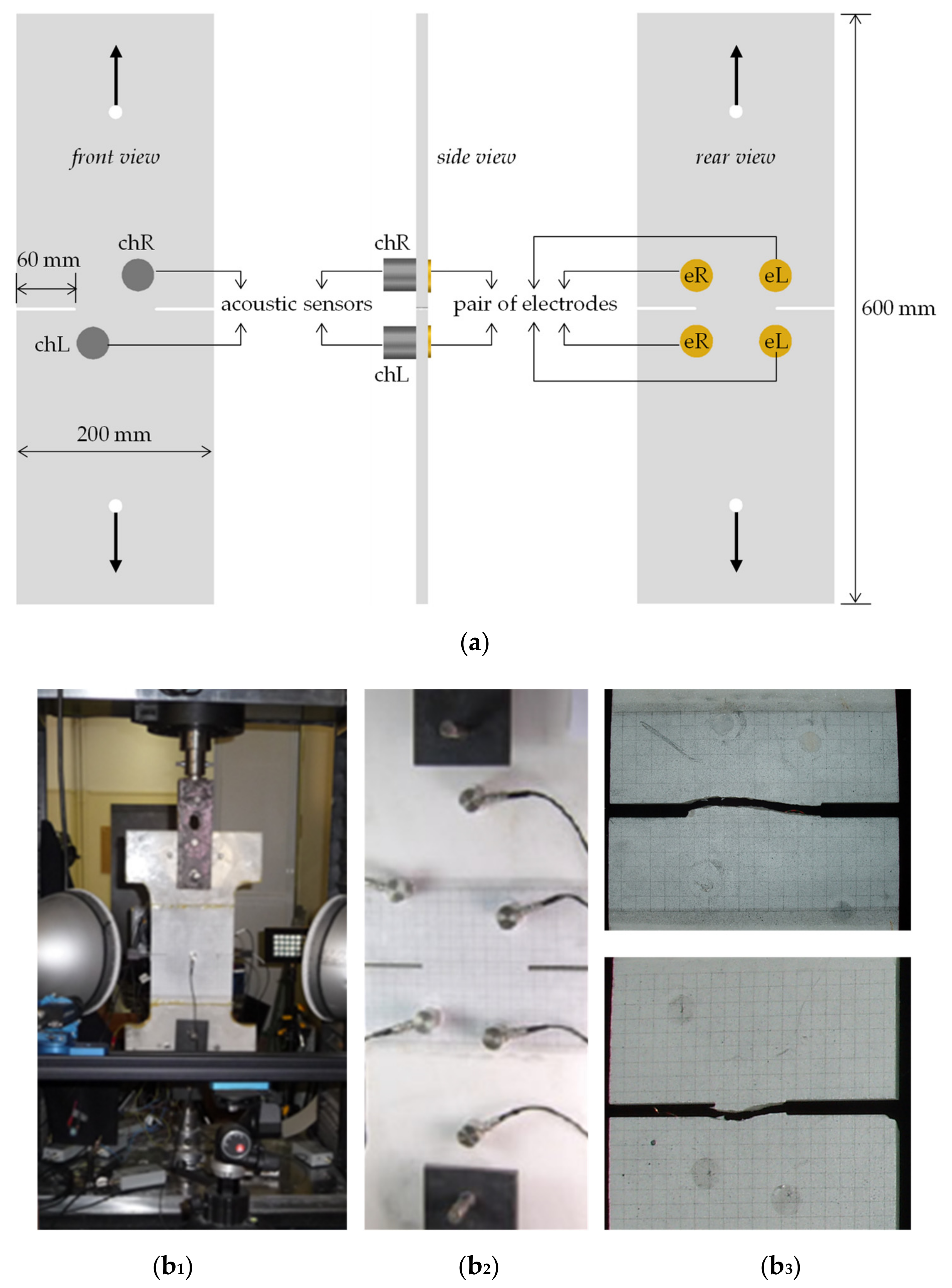
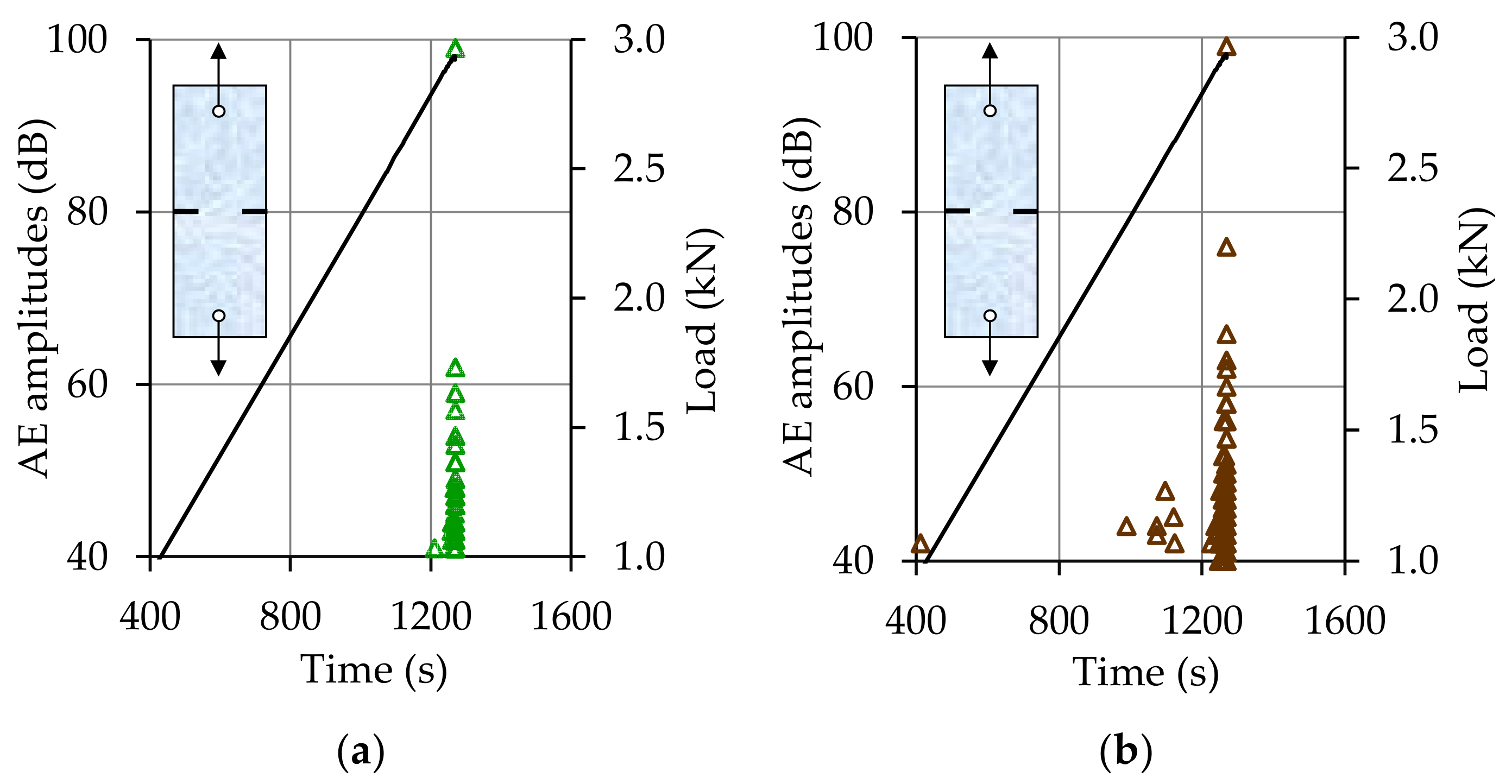
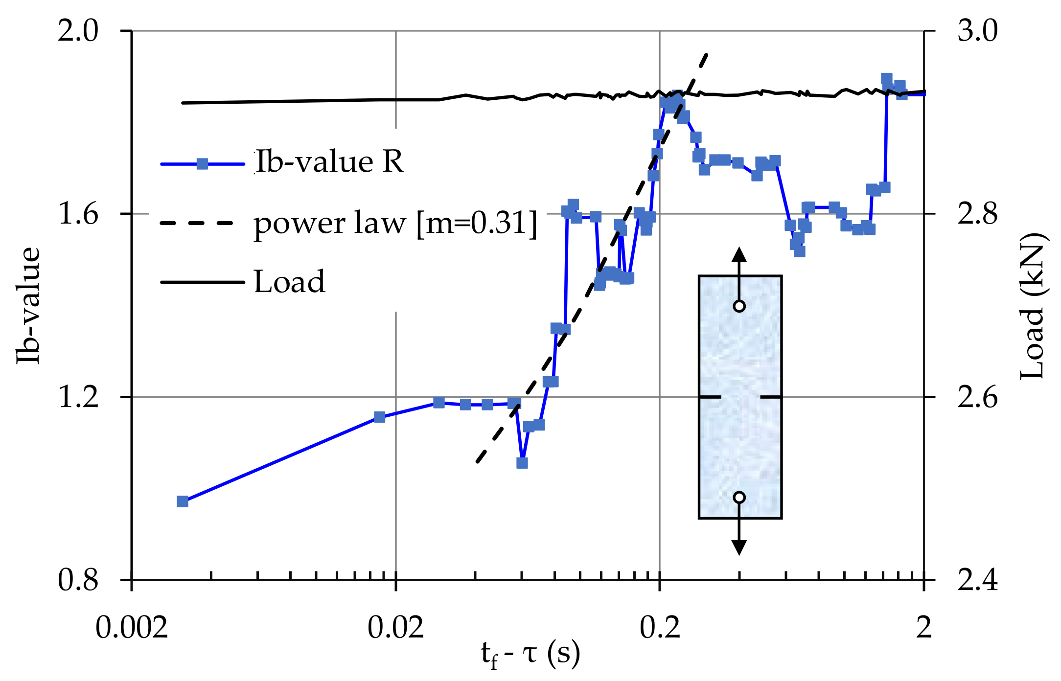
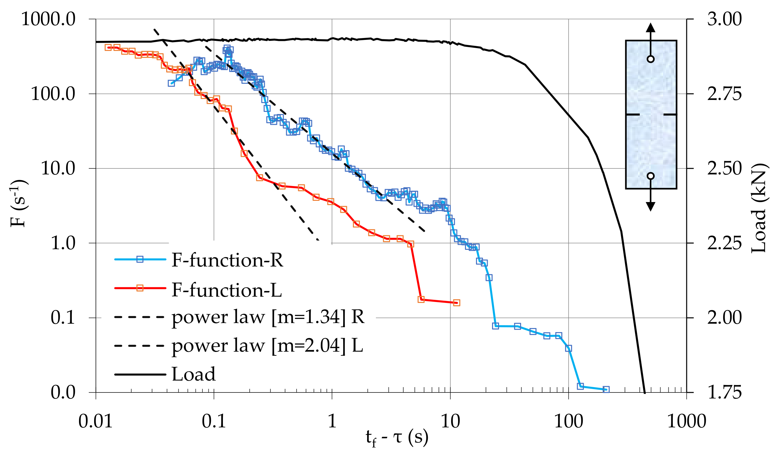
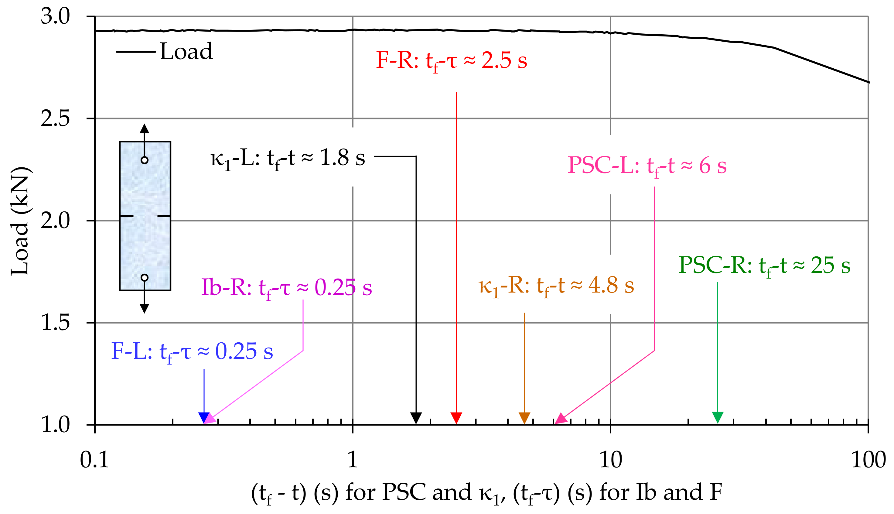
3.1. Direct Tension of Symmetrically Notched Marble Plates

Plate-shaped specimens, made of Dionysos marble, were submitted to uniaxial tension. Their geometry and dimensions and the experimental set-up are shown in Figure 3. Their thickness was 12 mm and two notches, symmetric with respect to the loading axis, were mechanically machined at both sides of the specimens. The depth of the notches was equal to a = 60 mm while their width was equal to 3 mm. An MTS Insight electro mechanical loading frame (capacity 10 kN) was used, adopting displacement-control conditions, at a constant rate equal to about 3 μm/s, ensuring, a quasi-static loading scheme.

At this point it must be highlighted that the characteristics of the experimental apparatus recording the AEs are of major importance in order to ensure the validity of the AE data. Concerns are reported in literature regarding the accuracy of electromechanical systems and the influence of EMI/RFI and temperature on their performance [70]. In this study.

AE data were analyzed by R15α piezoelectric acoustic sensors (the same type is used for both protocols discussed), denoted as chR and chL (see Figure 3a), which were properly attached in the vicinity of the crowns of the notches at the front side of the specimens (during the protocol additional sensors were employed in an attempt to exclude parasitic signals and, also, to enlighten the potential role of the anisotropic nature of Dionysos marble [71,72,73]).

The R15α sensors are considered as narrowband with resonance frequency 150 kHz and according to the manufacturer show a functional bandwidth that ranges from 50 kHz to 400 kHz, which proved to be suitable for the experiments using the specific protocols. The mounting surface of each sensor is ceramic, ensuring electrical isolation and circular with 19 mm radius which is significantly smaller than the size of the specimens ensuring in this way proper coupling. It must be noted that the ceramic surface that is firmly mounted on the specimen is the only surface of the sensor that is connected to the sensing piezoelectric crystal and can sense the AE. Provided the bandwidth of the AE sensors and the attenuation rate beyond the cutoff frequencies (i.e., more than 40 dB/decade) acoustic emissions that originate outside the experimental setup cannot be easily captured and influence the experimental data. Furthermore, according to the manufacturer (Physical Acoustics Corp.) the sensor’s functional temperature ranges from −65 °C up to 175 °C. In conclusion, the AE sensors used for both protocols ensure the data validity and reliability of the extracted results. The AE sensors are connected to 40 dB preamplifier stages (model 2/4/6, Physical Acoustics Corp.) enabled with 4th order analogue band-pass filters to further diminish any external noise. The captured signals are driven to a high sampling rate (40 MSample/s), two-channel data acquisition card (model PCI-2, Physical Acoustic Corp.) that is low-noise engineered and based on a high resolution (18 bit) A/D converter. However, and in spite of the aforementioned precautions, it is to be accepted that the problem of noise interference during SHM by means of acoustic or electrical signals is not in general solved. This is the reason that delays (if not prohibits) the safe in situ application of the procedures described here for the detection of pre-failure indices in large-scale structures, already in function. The issue is still under intensive investigation worldwide [70,74] due to its increased practical interest for the community of structural engineers.

For the detection of the PSC, two pairs of cyclically-shaped electric contacts (denoted as eR and eL), made of copper, were attached on the rear side of the specimens, again in the vicinity of the crowns of the two notches (Figure 3a). To record the PSC two sensitive programmable electrometers were used (model 6517A, Keithley). The main electrometer characteristic is the high accuracy of the order of 1% + 30 counts for electrical currents lower than 2 pA. The electrometer is capable of recording electrical currents varying from 3 fA up to 21 mA, approximately. The copper electrodes are connected to the electrometer using low-noise Keithley triax cables that were firmly placed during the experimental procedure in order to minimize any possible tribo-electric effects.

Before the application of any external loading both the sensing systems were set in order to ensure that no external noise is recorded. The electrometer according to the manufacturer must be allowed to restore to a background level after initializing for a warm up period of at least 1 hour. After this period of time, the zero set/correct procedure is followed for the PSC. The mechanical load is applied only when both the ACL regarding the AE and the electrical current regarding the PSC are found in low levels.

The loading system provides an analog voltage output linearly related to the applied mechanical load. This output of the MTS frame is provided as input to the AE high input impedance parametric port and to the corresponding PSC high input impedance data acquisition card. This action was performed during the experiments in order to pay special attention to the data synchronization. For all experiments described in this study, the equipment of the AE- and PSC-techniques started recording at the same time instant. For most accurate synchronization, the outcome of the applied load channel was continuously recorded not only by the internal system of the loading frame but also by both the AE and PSC systems. Only after the completion of each experiment are the data extracted from the: (a) loading frame system, (b) AE acquisition system, and (c) PSC recording system, and are further elaborated to extract the pre-failure criticality indices.

The temporal evolution of the amplitudes of the AEs recorded during a typical experiment of this protocol is shown in Figure 4a,b. The overall duration of the specific experiment was equal to about 1300 s. It can be seen clearly from these figures that the acoustic activity is intensified only during the very last interval of the loading processes, i.e., after the time instant t = 1200 s, while the specimen is almost “silent” for the earlier loading stages. Moreover, the data recorded during this critical time interval are very closely “packed” to each other and thus it is possible that crucial information may be hidden. In this context, it is preferable to plot the data against the time-to-failure parameter, t_f-t (where t_f denotes the time instant corresponding to the macroscopic fracture of the specimen), along a logarithmic scale, obtaining thus an “enlarged” view to what happens during the very last seconds before fracture.

This approach is vividly seen in Figure 5, where the temporal evolution of the Ib-value, calculated from the data provided by the acoustic sensor attached at the crown of the notch from which fracture finally started, is plotted against the t_fȒτ parameter together with the respective evolution of the load applied. The sliding “window” used to calculate the Ib-value included 50 consecutive hits.

It is seen from Figure 5 that at the instant t_fȒτ = 0.25 s (i.e., about 0.25 s before macroscopic fracture) and while the load is already stabilized almost at its maximum value, the Ib-value starts decreasing (with some strong fluctuations) from an initial value of about Ib ≈ 1.85 towards the value considered as critical, i.e., the value Ib ≈ 1.0. The fluctuations could be attributed to the transversely isotropic nature of the variety of marble used in the specific experimental protocol.

Proper fitting of the data corresponding to the decreasing branch of the Ib = Ib (t_fȒτ) plot indicates that they obey a power law described as:

$$Ib(t_f-\tau )=A_{Ib}·{(t_f-\tau )}^m$$

(13)

with m = 0.31.

From another perspective the acoustic activity is now described, for the same specimen, using the F-function. Advantage is taken of the data provided by both sensors, using a sliding “window” of 10 successive hits. The temporal variations of the F-function are plotted in Figure 6 against the t_fȒτ parameter (where τ is the average value of the time instants of occurrence of the hits comprising the sliding window) along a logarithmic scale, in juxtaposition to the respective evolution of the load applied.

As can be seen from Figure 6, the values of the F-function, calculated from the data of the sensor close to the crown of the notch from which macroscopic fracture started (blue line), increases steadily during the last 200 s of the test’s duration. What is more important, however, is that about 2.5 s before fracture the behaviour of the F-function is, again dictated (almost perfectly) by a power law of the following form:

$$F(t_f-\tau )=A_F·{(t_f-\tau )}^m$$

(14)

with m = 1.34.

The temporal evolution of the F-function calculated using the data of the second sensor (red line) is governed by the same law (with m = 2.04). The difference is that the validity of this law is now restricted to the time interval t_fȒτ < 0.25 s. This observation could be interpreted as follows: The damage mechanisms which became dominant when the specimen is about to enter into its critical stage, a fact that is somehow designated by the onset of validity of the above power law, have been activated much earlier in the close vicinity of the crown from which the fracture started.

Exploring the acoustic activity, for the same specimen as above, in terms of the natural time concept, the temporal evolution of the natural time parameters (i.e., the variance κ₁ and the entropy S and the entropy under time reversal S_) is plotted in Figure 7 for the data regarding the energy of the hits, provided by the sensor closer to the crown of the notch from which macroscopic fracture began. The plot is realized against the t_f-t parameter adopting a semi-logarithmic manner, together with the respective evolution of the load. In the same figure, two dashed lines parallel to the t_f-t axis are drawn, corresponding to the critical values κ₁ = 0.07 and S_u = 0.0966. It can be seen that all three criticality conditions (i.e., κ₁ = 0.070 and S, S_ ≤ 0.0966) are met, for the first time, during the interval from 3.4 s ≤ t_f-t ≤ 4.8 s, i.e., about 4.8 s before macroscopic fracture (see the yellow-shaded area in Figure 7) with the variance κ₁ approaching and briefly fluctuating around the critical value 0.070 while both S and S_ remain lower than 0.0966.

The respective data obtained by the second acoustic sensor (i.e., the one close to the notch from which the onset of macroscopic fracture was delayed) can be seen in Figure 8. A behaviour similar to that shown in Figure 7 for the parameters κ₁, S, S_ is seen. In this case, with respect to the previously discussed time delay, the first time all three criticality conditions (i.e., κ₁ = 0.070 and S, S_ ≤ 0.0966) are met, is during the 1.4 s ≤ t_f-t ≤ 1.8 s time interval, i.e., about 1.8 s before the macroscopic fracture (see the yellow area in Figure 8).

In order now to explore the electrical activity, for the same as previously specimen, the PSCs recorded by the two electric sensors are presented in Figure 9, against the t_f-t parameter adopting a semi-logarithmic manner, together with the respective data for the load applied. It is evident from Figure 9 that the temporal evolution of the PSC recorded by the sensor close to the notch from which macroscopic fracture began (blue line), starts obeying a power law of the following form:

$$PSC(t_f-t)=A_{PSC}·{(t_f-t)}^m$$

(15)

at about 25 s before fracture (namely at the instant with t_f-t ≈ 25 s), i.e., much earlier compared to the previous parameters. The exponent m is now equal to m = 0.48. The PSC recorded by the second sensor (red line) is significantly weaker for the whole duration of the experiment, and starts obeying the above power law (with m = 0.52) at about 6 s before fracture, i.e., with a considerable delay, with respect to the other sensor. The existence of the power law is indicative of a system’s entrance into criticality. Therefore, the fact that a power law firstly emerges from the PSC signal recorded by the sensor closer to the notch from which the catastrophic fracture started, is in full accordance with previously reported results [9,18,69].

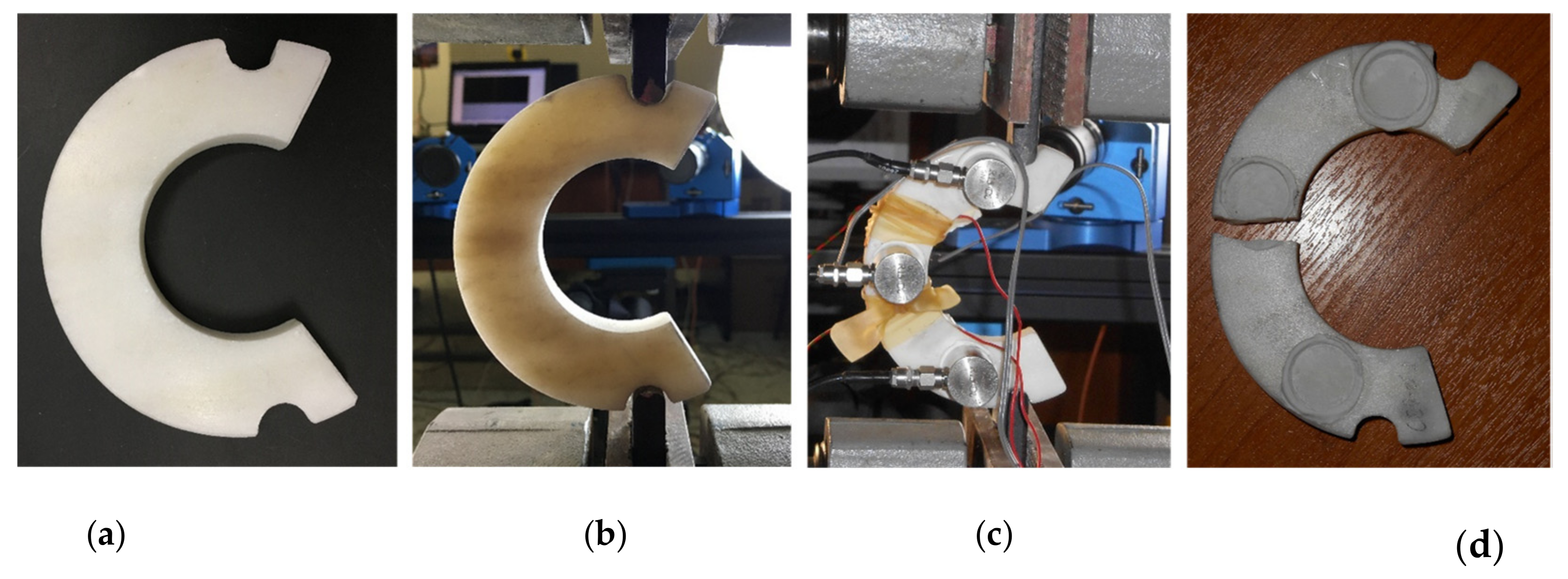
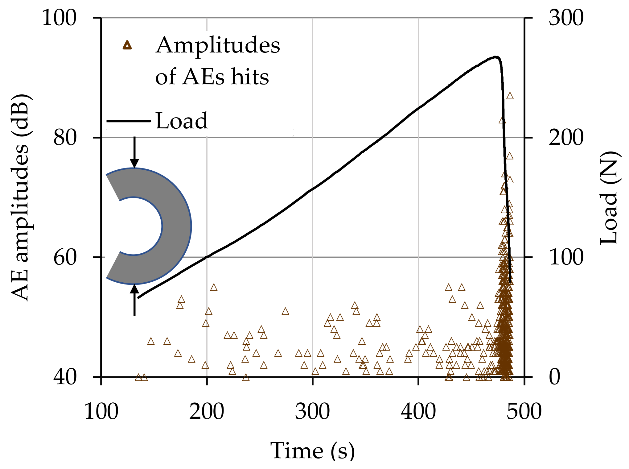
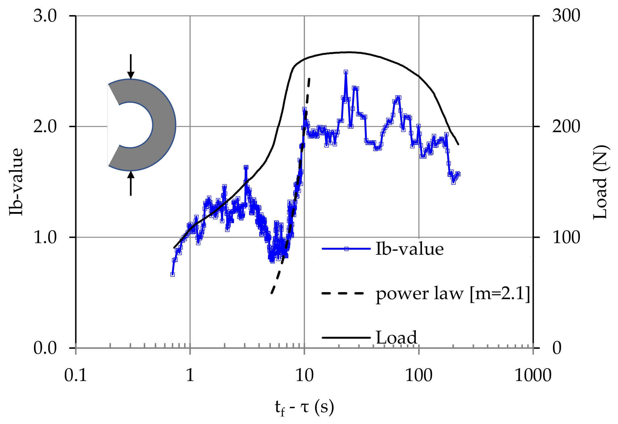
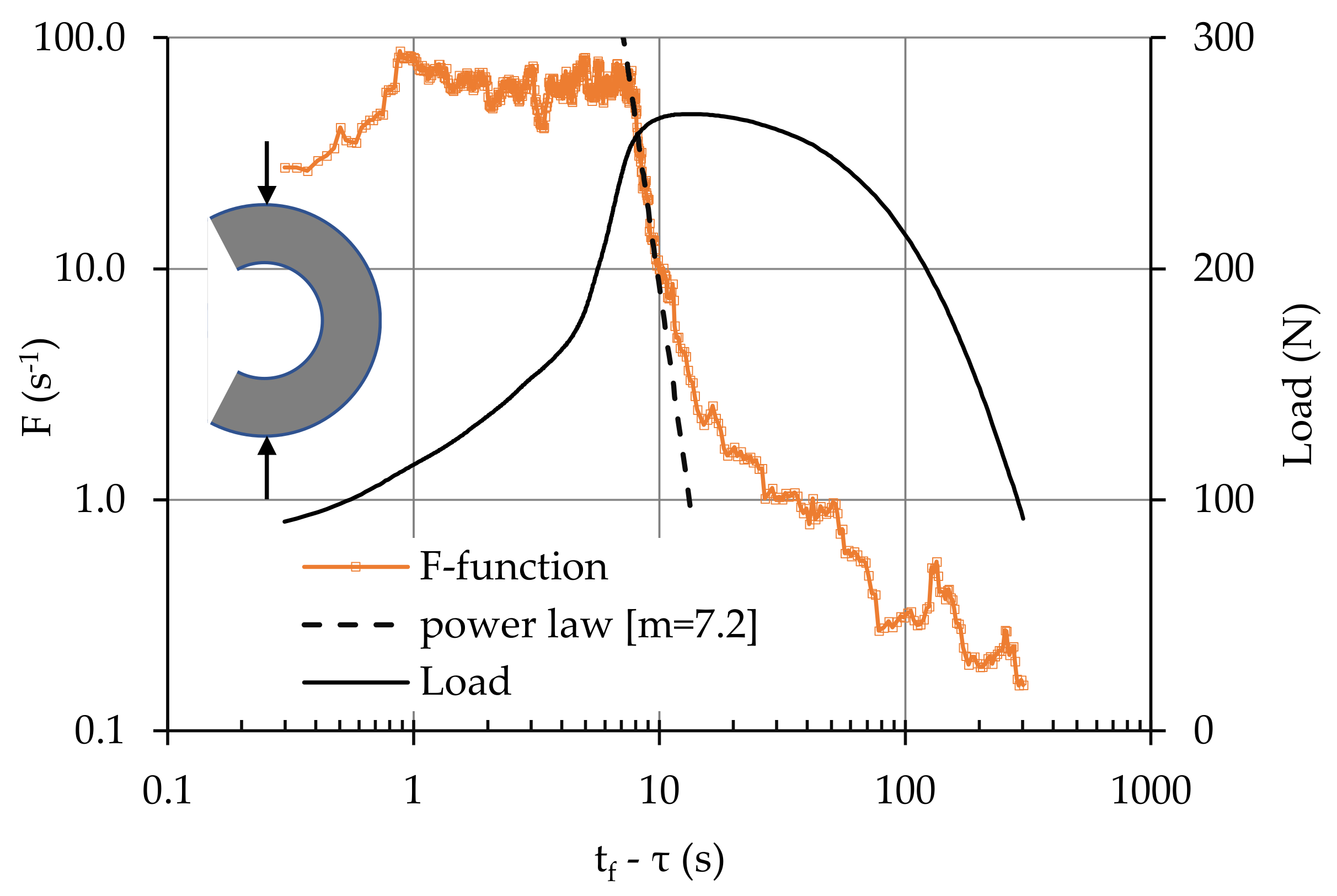
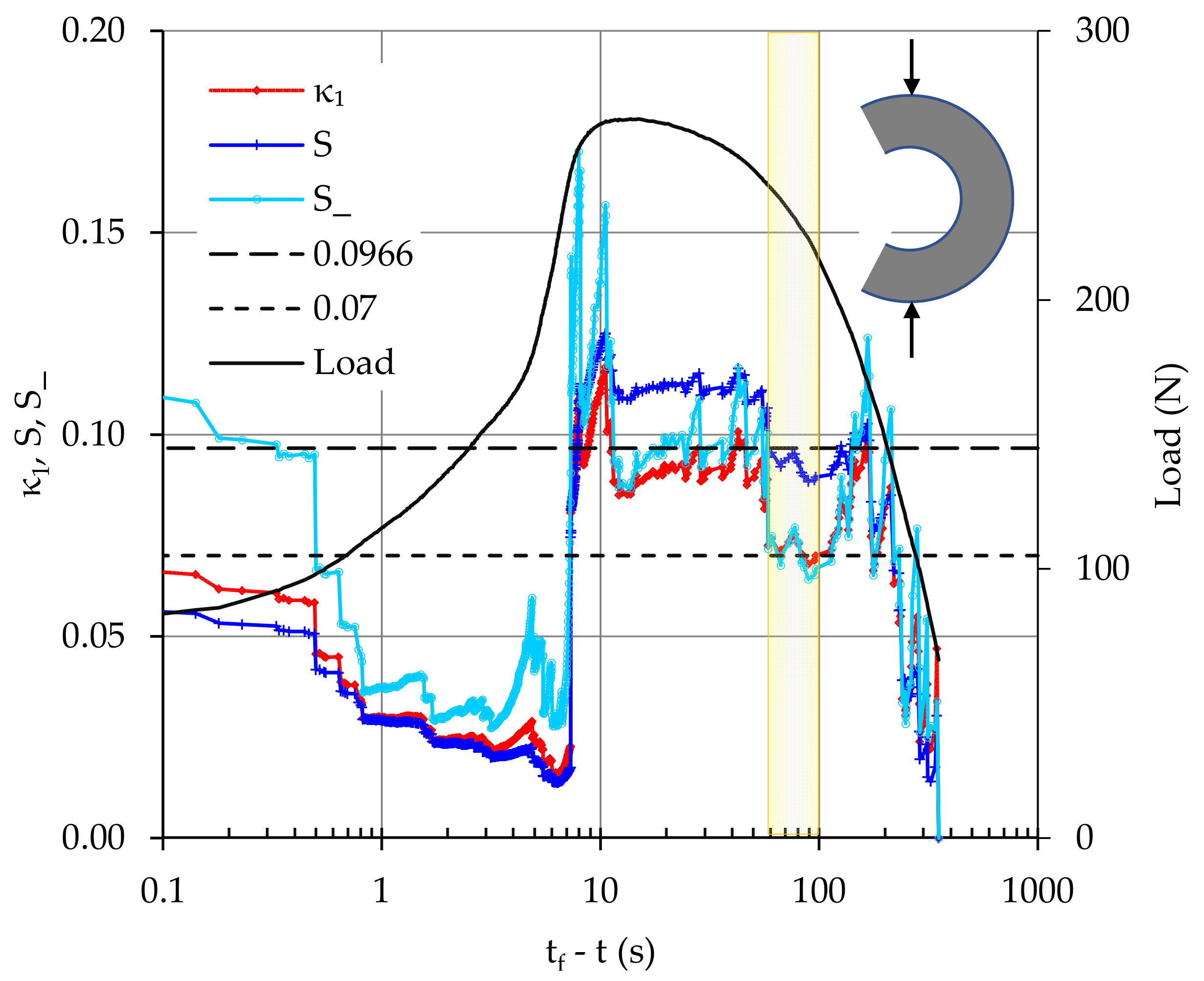
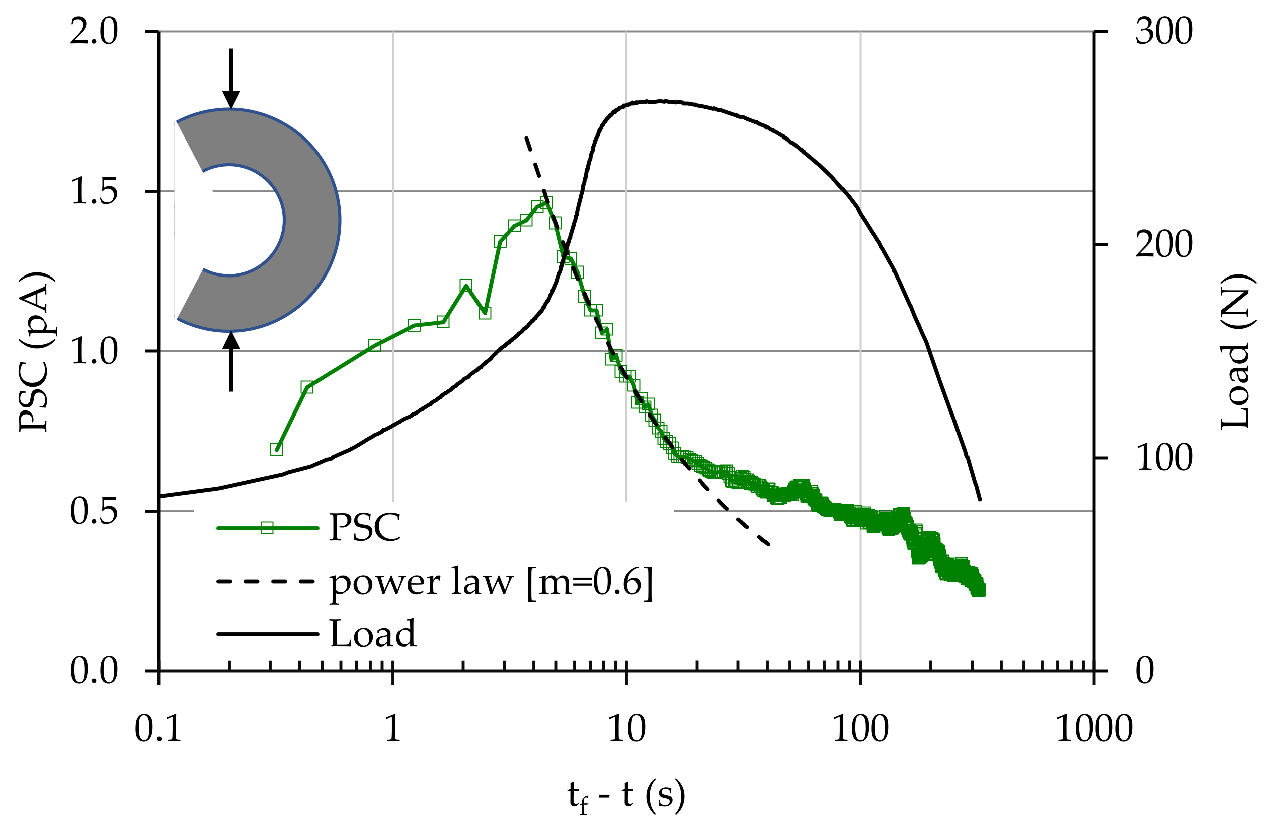
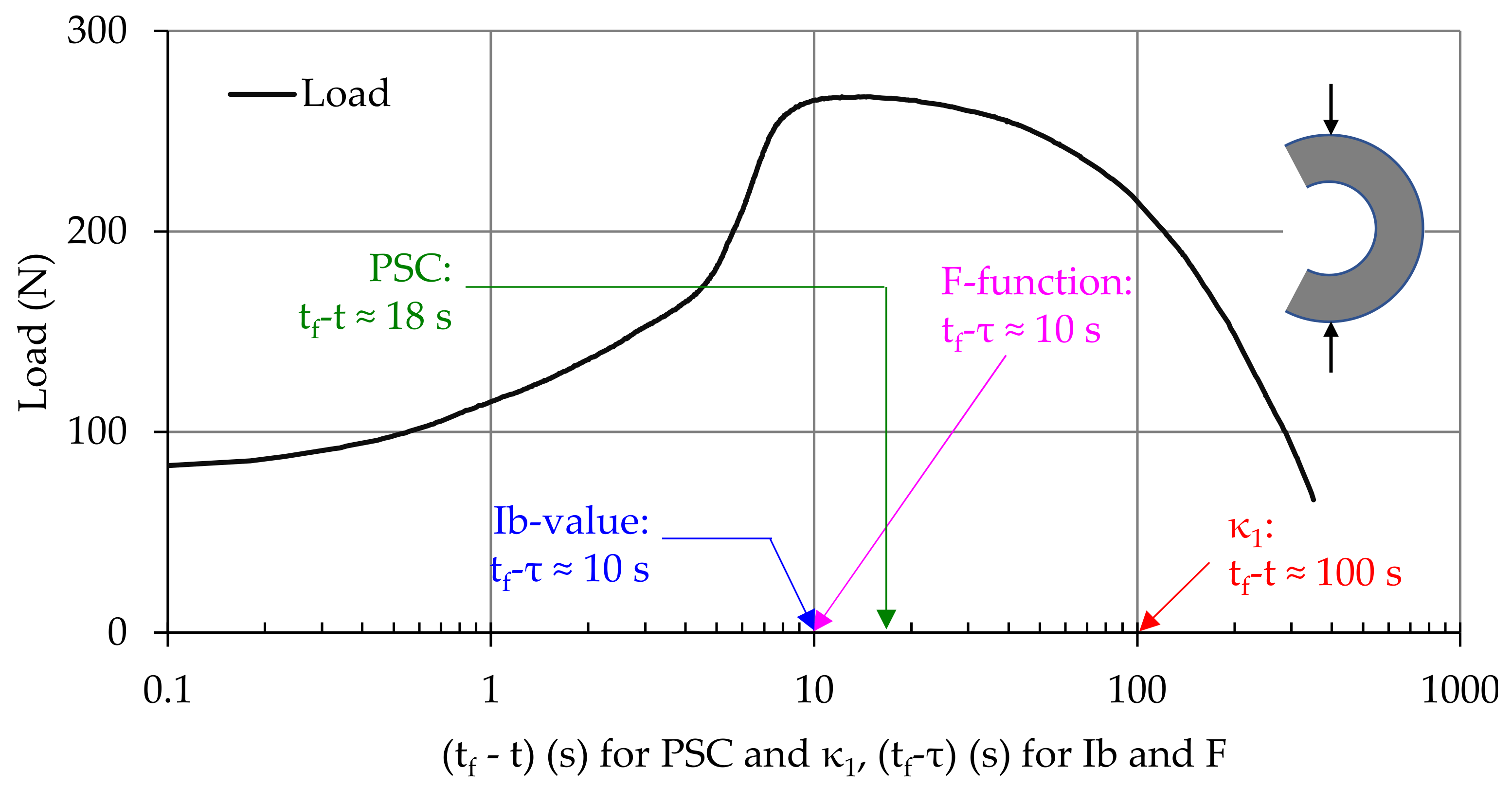
3.2. Diametral Compression of Circular Semi Rings

Dionysos marble was used for the preparation of the specimens of the present protocol. They were shaped in the form of CSRs, according to the configuration proposed by Markides et al. [75,76] for the indirect determination of the tensile strength of brittle geomaterials. The geometry of the specimens is shown in Figure 10. Their outer and inner diameters were equal to 100 mm and 50 mm, respectively while the thickness was equal to 10 mm.

The specimens were loaded under diametral compression (using two rods placed in two grooves sculptured at the specimen’s outer periphery) by means of an electromechanical Insight loading frame of capacity 10 kN. Displacement-control loading conditions were chosen for all the tests at a rate of 0.02 mm/min, ensuring again quasi-static loading of the specimens. Data from an R15α acoustic sensor, properly attached in the central area of the specimens (Figure 10) were analyzed. Two additional sensors, attached in the vicinity of the load transfer system were used to detect parasitic signals. Moreover, a pair of rectangular electric contacts, made of copper, was properly attached at the central region of all specimens (i.e., in the area where fracture is expected), to record the PSC (Figure 10). For a typical specimen that was prepared for testing, the experimental set-up and a fractured specimen are shown in Figure 11.

The temporal evolution of the amplitudes of the AEs recorded during a typical experiment with a CSR specimen is shown in Figure 12. The overall duration of the specific experiment is equal to about 480 s. Although in this case acoustic signals are recorded almost from the very beginning of the experiment, it is clear that the acoustic activity is intensified only during the very last interval of the loading processes, i.e., after the time instant t = 470 s, namely during the last 10 s of the experiment. It can be seen that during the above time interval (i.e., 470 < t < 480 s), the data recorded are again extremely densely “packed” and, thus, it was again decided to plot them against the time-to-failure parameter, t_fȒτ or t_f-t, along the logarithmic scale, paying attention to the last seconds before fracture (adopting the procedure presented while describing the previous protocol with marble plates under tension). In this direction, the temporal variation of the Ib-value is presented (again using a sliding “window” of 50 successive hits) against the t_fȒτ parameter together with the respective evolution of the load applied in Figure 13. In agreement with the observations of the previous protocol, the Ib-value fluctuates at the level with Ib ≈ 2 s for about 200 s before the specimen’s fracture. Then at the instant t_fȒτ ≈ 10 s (while the load applied has already attained its maximum value) a descending branch is observed and the Ib-value tends to the critical level Ib = 1.0, attained at about 7 s before fracture. The evolution of the Ib-values during this descending branch is fitted excellently by the power law given in Equation (13) with an exponent m equal to m = 2.1.

The temporal evolution of the F-function for the CSR specimen as above, is plotted in Figure 14 (using a sliding “window” with 15 consecutive hits), versus the t_fȒτ parameter. It can be seen that the qualitative agreement with the plot of the Ib-value is excellent. At about 10 s before fracture the F-function starts obeying the power law of Equation (14) with m = 7.2 until the t_fȒτ = 7 s. Then its value is stabilized at a level with F ≈ 90 s⁻¹ until about 1 s before fracture, and then it decreases.

In terms of the natural time concept, the temporal variation of the parameters κ₁, S and S_, for the same CSR specimen, is plotted in Figure 15 against the t_f-t parameter along semi-logarithmic scale, together with the respective evolution of the applied load. It can be seen from Figure 15 that a first critical stage is detected at the time interval between t_f-t ≈ 100 s until t_f-t ≈ 60 s, i.e., about 100 s before macroscopic fracture (yellow-shaded area in Figure 15), with the variance κ₁ crossing and eventually fluctuating around the critical value of 0.070 with both entropies S, S_ remaining lower than S_u = 0.0966.

The electrical activity, for the specific specimen, is explored now in terms of the PSC recorded versus the t_f-t parameter, adopting a semi-logarithmic manner, together with the respective evolution of the applied load (Figure 16). It can be seen from this figure that the temporal evolution of the PSC obeys the power law of Equation (15) from the time instant t_f-t ≈ 18 s until the instant t_f-t ≈ 5 s. The exponent m is now equal to m = 0.60. Then the PSC decreases steadily until the specimen’s macroscopic fracture.

4. Discussion and Concluding Remarks

The acoustic and electrical activities in mechanically loaded marble specimens were explored in order to detect and comparatively assess pre-failure indicators provided by the temporal evolution of three formulations for the acoustic activity (the Ib-value, the F-function, and the parameters κ₁, S, S_ of the natural time) and the pressure-stimulated currents for the electrical activity. Both activities were explored in terms of the time-to-failure parameter and attention was paid to the loading stages close to the instant that the applied load tends to its maximum value, i.e., while the specimens are entering into their critical stage, that of impending macroscopic fracture.

Data from two experimental protocols were analyzed: direct tension of symmetrically notched marble plates and compression of marble circular semi-rings. In spite of the different geometries and the different loading schemes, the temporal evolution of the electrical and the acoustic activities for the specimens of both protocols exhibited some interesting common characteristics. The most striking one is, perhaps, that during the last loading steps the time dependence of the Ib-value, the F-function and the PSC is described by a common power law. It is reasonable to assume that the onset of validity of this power law designates some differentiation of the damage mechanisms activated within the loaded specimen, mechanisms that will eventually cause its final destruction. Therefore, the onset of validity of this power law could be considered as a proper indicator warning about upcoming fracture, i.e., a pre-failure index.

A comprehensive insight of the time instants, at which the pre-failure indicators are detected according to each one of the parameters considered, is gained from Figure 17. In this figure the temporal variation of the applied load is plotted, and, simultaneously the time instants at which the pre-failure indicators are detected by each one of the four parameters analyzed are depicted, for the typical specimen of the protocol with marble plates under tension. It can be seen from this figure that the above warning signals are detected within a relatively narrow time interval (compared to the test’s duration, which was equal to about 1300 s) of about 25 s before the specimen’s macroscopic fracture. Comparatively speaking, it can be concluded that for the specific specimen the electrical activity, as it is expressed by the PSC recorded, provides its warning signal earlier, while the signal obtained from the temporal variation of the Ib-value is the one most delayed. It is also worth mentioning that in the specific protocol two sensors were used for both the electrical and acoustic activities. In this context it was systematically observed, for all the specimens of the protocol, that the electrical and the acoustic activities are much more intense in the immediate vicinity of the crown of the notch from which fracture began and that the power law starts dictating the response of this specific area of the specimen much earlier.

Similar conclusions are drawn from the respective data provided by the protocol with the CSR specimens, which are plotted in Figure 18. The main difference is that now the natural time analysis provides the earliest warning signal. The time instant at which the electrical activity provides the warning signal is quite close to those provided by the F-function and the Ib-value.

Before concluding, it is emphasized that this study is based on a limited number of experimental protocols with specimens made of marble. It is quite obvious that additional experimental protocols, with a wider variety of loading types and materials, must be analyzed before definite conclusions are drawn. In any case, this preliminary comparative study indicates that both the electrical and the acoustic activity capture the differentiation of the damage mechanisms during the last loading steps before the specimen’s macroscopic fracture.

It could be anticipated at this point that the time instants at which the specific pre-failure indicators are detected are very close to the instant of catastrophic fracture, preventing reactive actions and, thus, limiting their practical applicability. Although this is the case one should keep in mind that this is a preliminary study and it is quite possible that more sophisticated arrangements of the respective sensors by means, for example, of a proper grid arrangement, could provide earlier pre-failure indicators rendering their practical application more attractive.

What is to be explored next is which parameter is the most efficient, or in other words which one of the quantities used to describe the electrical and acoustic activities provides more systematically and earlier the respective pre-failure indicators. Obviously, besides the four parameters considered here, one could investigate the temporal evolution of additional ones, like for example, the energy content, the power of the electric and acoustic signals, or the Euclidean distance between the sources, provided by the electric and acoustic signals. For the latter in particular, i.e., the three-dimensional Euclidean distance between the sources of the acoustic signals, already available data have proven encouraging [77].

References

1. Grosse, C.U.; Ohtsu, M. (Eds.) Acoustic Emission Testing; Springer: Berlin/Heidelberg, Germany, 2008. [Google Scholar]
2. Ohtsu, M. The history and development of acoustic emission in concrete engineering. Mag. Concr. Res. 1996, 48, 321–330. [Google Scholar] [CrossRef]
3. Behnia, A.; Chai, H.K.; Shiotani, T. Advanced structural health monitoring of concrete structures with the aid of acoustic emission. Constr. Build. Mater. 2014, 65, 282–302. [Google Scholar] [CrossRef]
4. Varotsos, P.A. The Physics of Seismic Electric Signals; TerraPub: Tokyo, Japan, 2005. [Google Scholar]
5. Varotsos, P.A.; Sarlis, N.V.; Skordas, E.S. Attempt to distinguish electric signals of a dichotomous nature. Phys. Rev. E 2003, 68, 031106. [Google Scholar] [CrossRef] [PubMed] [Green Version]
6. Surkov, V.; Hayakawa, M. Laboratory Study of Rock Deformation and Fracture. In Ultra and Extremely Low Frequency Electromagnetic Fields; Springer Geophysics: Tokyo, Japan, 2014; pp. 335–372. [Google Scholar]
7. Vallianatos, F.; Triantis, D.; Tzanis, A.; Anastasiadis, C.; Stavrakas, I. Electric earthquake precursors: From laboratory results to field observations. Phys. Chem. Earth 2004, 29, 339–351. [Google Scholar] [CrossRef]
8. Aggelis, D.G.; Soulioti, D.V.; Sapouridis, N.; Barkoula, N.M.; Paipetis, A.S.; Matikas, T.E. Acoustic emission characterization of the fracture process in fibre reinforced concrete. Constr. Build. Mater. 2011, 25, 4126–4131. [Google Scholar] [CrossRef]
9. Kourkoulis, S.K.; Pasiou, E.D.; Dakanali, I.; Stavrakas, I.; Triantis, D. Notched marble plates under tension: Detecting pre-failure indicators and predicting entrance to the “critical stage”. Fatigue Fract. Eng. Mater. Struct. 2018, 41, 776–786. [Google Scholar] [CrossRef]
10. Shearer, P.M. Introduction to Seismology; Cambridge University Press: Cambridge, UK, 1999; pp. 1–189. [Google Scholar]
11. Colombo, S.; Main, I.G.; Forde, M.C. Assessing damage of reinforced concrete beam using ‘‘b-value’’ analysis of acoustic emission signals. J. Mater. Civ. Eng. 2003, 15, 280–286. [Google Scholar] [CrossRef] [Green Version]
12. Vallianatos, F.; Michas, G.; Hloupis, G. Seismicity patterns prior to the Thessaly (Mw6. 3) strong earthquake on 3 March 2021 in terms of multiresolution wavelets and natural time analysis. Geosciences 2021, 11, 379. [Google Scholar] [CrossRef]
13. Contoyiannis, Y.F.; Potirakis, S.M.; Diakonos, F.K. Wavelet-based detection of scaling behavior in noisy experimental data. Phys. Rev. E 2020, 101, 052104. [Google Scholar] [CrossRef]
14. Varotsos, P.A.; Sarlis, N.V.; Skordas, E.S. Natural Time Analysis: The New View of Time: Precursory Seismic Electric Signals, Earthquakes and Other Complex Time Series; Springer: Heidelberg, Germany, 2011. [Google Scholar]
15. Varotsos, P.A.; Sarlis, N.V.; Skordas, E.S.; Tanaka, H.K.; Lazaridou, M.S. Entropy of seismic electric signals: Analysis in natural time under time reversal. Phys. Rev. E 2006, 73, 0311144. [Google Scholar] [CrossRef] [Green Version]
16. Tsallis, C. Possible generalization of Boltzmann-Gibbs statistics. J. Stat. Phys. 1988, 52, 479–487. [Google Scholar] [CrossRef]
17. Tsallis, C. Nonadditive entropy Sq and nonextensive statistical mechanics: Applications in geophysics and elsewhere. Acta Geophys. 2012, 60, 502–525. [Google Scholar] [CrossRef]
18. Triantis, D.; Pasiou, E.D.; Stavrakas, I.; Kourkoulis, S.K. Hidden affinities between electric and acoustic activity in brittle materials at near-fracture load levels. Rock Mech. Rock Eng. 2022, 1–18. [Google Scholar] [CrossRef]
19. Tzanis, A.; Vallianatos, F. Distributed power-law seismicity changes and crustal deformation in the SW Hellenic ARC. Nat. Hazards Earth Syst. Sci. 2003, 3, 179–195. [Google Scholar] [CrossRef]
20. Iowa State University, Nondestructive Evaluation Technique: History of Acoustic Emission Testing. Available online: https://www.nde-ed.org/NDETechniques/AcousticEmission/AE_History.xhtml (accessed on 8 December 2021).
21. Kishinouye, F. An experiment on the progression of fracture. (A preliminary report). Jisin 6:24-31(1934) translated and published by Ono K. J. Acoust. Emiss. 1990, 9, 177–180. [Google Scholar]
22. Förster, F. Akustische untersuchung der bildung von martensitnadeln (Acoustic study of the formation of martensile needels). Z. Für Met. 1936, 29, 245. [Google Scholar]
23. Kaiser, E. A Study of Acoustic Phenomena in Tensile Test. Ph.D. Thesis, Technical University of Munich, Munich, Germany, 1950. [Google Scholar]
24. Grosse, C.U.; Ohtsu, M.; Aggelis, D.G.; Shiotani, T. (Eds.) Acoustic Emission Testing: Basics for Research-Applications in Engineering; Springer Nature: Cham, Switzerland, 2021. [Google Scholar]
25. Sause, M.G.R. In Situ Monitoring of Fiber-Reinforced Composites: Theory, Basic Concepts, Methods, and Applications; Springer: Berlin/Heidelberg, Germany, 2016. [Google Scholar]
26. Mohammad, I.; Huang, H. Monitoring fatigue crack growth and opening using antenna sensors. Smart Mater. Struct. 2010, 19, 055023. [Google Scholar] [CrossRef] [Green Version]
27. Sharma, S.K.; Sivarathri, A.K.; Chauhan, V.S.; Sinapius, M. Effect of low temperature on electromagnetic radiation from soft PZT SP-5A under impact loading. J. Electron. Mater. 2018, 47, 5930–5938. [Google Scholar] [CrossRef]
28. Stavrakas, I.; Anastasiadis, C.; Triantis, D.; Vallianatos, F. Piezo stimulated currents in marble samples: Precursory and concurrent-with-failure signals. Nat. Hazards Earth Syst. Sci. 2003, 3, 243–247. [Google Scholar] [CrossRef] [Green Version]
29. Kyriazopoulos, A.; Anastasiadis, C.; Triantis, D.; Brown, C.J. Non-destructive evaluation of cement-based materials from pressure-stimulated electrical emission—Preliminary results. Constr. Build. Mater. 2011, 25, 1980–1990. [Google Scholar] [CrossRef] [Green Version]
30. Enomoto, J.; Hashimoto, H. Emission of charged particles from indentation fracture of rocks. Nature 1990, 346, 641–643. [Google Scholar] [CrossRef]
31. Ogawa, T.K.; Miura, T. Electromagnetic radiation from rocks. J. Geophys. Res. 1985, 90, 6245–6249. [Google Scholar] [CrossRef]
32. Archer, J.W.; Dobbs, M.R.; Aydin, A.; Reeves, H.J.; Prance, R.J. Measurement and correlation of acoustic emissions and pressure stimulated voltages in rock using an electric potential sensor. Int. J. Rock Mech. Min. 2016, 89, 26–33. [Google Scholar] [CrossRef] [Green Version]
33. Niu, Y.; Wang, C.J.; Wang, E.Y.; Li, Z.H. Experimental study on the damage evolution of gas-bearing coal and its electric potential response. Rock Mech. Rock Eng. 2019, 52, 4589–4604. [Google Scholar] [CrossRef]
34. Triantis, D.; Anastasiadis, C.; Stavrakas, I. The correlation of electrical charge with strain on stressed rock samples. Nat. Hazards Earth Syst. 2008, 8, 1243–1248. [Google Scholar] [CrossRef] [Green Version]
35. Zhang, X.; Li, Z.H.; Niu, Y.; Cheng, F.Q.; Ali, M.; Bacha, S. An experimental study on the precursory characteristics of EP before sandstone failure based on critical slowing down. J. Appl. Geophys. 2019, 170, 103818. [Google Scholar] [CrossRef]
36. Whitworth, R.W. Charged dislocations in ionic crystals. Adv. Phys. 1975, 24, 203–304. [Google Scholar] [CrossRef]
37. Varotsos, P.A.; Sarlis, N.V.; Skordas, E.S. Long-range correlations in the electric signals that precede rupture. Phys. Rev. E 2002, 66, 011902. [Google Scholar] [CrossRef] [Green Version]
38. Saltas, V.; Vallianatos, F.; Triantis, D.; Stavrakas, I. Complexity in Laboratory Seismology: From Electrical and Acoustic Emissions, to Fracture. In Complexity Measurement and Application to Seismic Time Series, Measurement and Application; Elsevier: Amsterdam, The Netherlands, 2008; pp. 239–273. [Google Scholar]
39. Takeuchi, A.; Aydan, Ö.; Sayanagi, K.; Nagao, T. Generation of electromotive force in igneous rocks subjected to non-uniform loading. Earthq. Sci. 2011, 24, 593–600. [Google Scholar] [CrossRef] [Green Version]
40. Slifkin, L. Seismic electric signals from displacement of charged dislocations. Tectonophysics 1993, 224, 149–152. [Google Scholar] [CrossRef]
41. Vallianatos, F.; Tzanis, A. On possible scaling laws between electric earthquake precursors (EEP) and earthquake magnitude. Geophys. Res. Lett. 1999, 26, 2013–2016. [Google Scholar] [CrossRef] [Green Version]
42. Sammonds, P.R.; Meredith, P.G.; Murrel, S.A.F.; Main, I.G. Modelling the damage evolution in rock containing pore fluid by acoustic emission. In Rock Mechanics in Petroleum Engineering; OnePetro: Delft, The Netherlands, 1994. [Google Scholar]
43. Shiotani, T.; Yuyama, S.; Li, Z.W.; Othsu, M. Quantitative Evaluation of Fracture Process in Concrete by the Use of Improved b-value. In 5th International Symposium Non-Destructive Testing in Civil Engineering; Uohoto, T., Ed.; Elsevier Science: Amsterdam, The Netherlands, 2000; pp. 293–302. [Google Scholar]
44. Triantis, D.; Kourkoulis, S.K. An alternative approach for representing the data provided by the acoustic emission technique. Rock Mech. Rock Eng. 2018, 51, 2433–2438. [Google Scholar] [CrossRef]
45. Zhang, J.Z.; Zhou, X.P.; Zhou, L.S.; Berto, F. Progressive failure of brittle rocks with non-isometric flaws: Insights from acousto-optic-mechanical (AOM) data. Fatigue Fract. Eng. Mater. Struct. 2019, 42, 1787–1802. [Google Scholar] [CrossRef]
46. Wang, X.; Wang, E.; Liu, X. Damage characterization of concrete under multi-step loading by integrated ultrasonic and acoustic emission techniques. Constr. Build. Mater. 2019, 221, 678–690. [Google Scholar] [CrossRef]
47. Yao, W.; Yu, J.; Liu, X.; Zhou, X.; Cai, Y.; Zhu, Y.L. Study on acoustic emission characteristics and failure prediction of post-high-temperature granite. J. Test. Eval. 2019, 48, 2459–2473. [Google Scholar] [CrossRef]
48. Ge, Z.; Sun, Q. Acoustic emission characteristics of gabbro after microwave heating. Rock Mech. Rock Eng. 2021, 138, 104616. [Google Scholar] [CrossRef]
49. Varotsos, P.A.; Sarlis, N.V.; Tanaka, H.K.; Skordas, E.S. Similarity of fluctuations in correlated systems: The case of seismicity. Phys. Rev. E 2005, 72, 041103. [Google Scholar] [CrossRef] [PubMed] [Green Version]
50. Uyeda, S.; Kamogawa, M.; Tanaka, H. Analysis of electrical activity and seismicity in the natural time domain for the volcanic-seismic swarm activity in 2000 in the Izu Island region, Japan. J. Geophys. Res. 2009, 114, B02310. [Google Scholar] [CrossRef] [Green Version]
51. Vallianatos, F.; Michas, G.; Papadakis, G. Non-extensive and natural time analysis of seismicity before the Mw6.4, 12 October 2013 earthquake in the South West segment of the Hellenic Arc. Physica A 2014, 414, 163–173. [Google Scholar] [CrossRef]
52. Varotsos, P.A.; Sarlis, N.V.; Skordas, E.S.; Lazaridou, M.S. Identifying sudden cardiac death risk and specifying its occurrence time by analyzing electrocardiograms in natural time. Appl. Phys. Lett. 2007, 91, 064106. [Google Scholar] [CrossRef]
53. Baldoumas, G.; Peschos, D.; Tatsis, G.; Chronopoulos, S.K.; Christofilakis, V.; Kostarakis, P.; Varotsos, P.; Sarlis, N.V.; Skordas, E.S.; Bechlioulis, A.; et al. A prototype photoplethysmography electronic device that distinguishes congestive heart failure from healthy individuals by applying natural time analysis. Electronics 2019, 8, 1288. [Google Scholar] [CrossRef] [Green Version]
54. Sarlis, N.V.; Skordas, E.S.; Varotsos, P.A. Heart rate variability in natural time and 1/f “noise”. Eur. Lett. 2009, 87, 18003. [Google Scholar] [CrossRef]
55. Sarlis, N.V.; Varotsos, P.A.; Skordas, E.S. Flux avalanches in YBa2Cu3O7−x films and rice piles: Natural time domain analysis. Phys. Rev. B 2006, 73, 054504. [Google Scholar] [CrossRef]
56. Vallianatos, F.; Michas, G.; Benson, P.; Sammonds, P. Natural time analysis of critical phenomena: The case of acoustic emissions in triaxially deformed Etna basalt. Physica A 2013, 392, 5172–5178. [Google Scholar] [CrossRef]
57. Hloupis, G.; Stavrakas, I.; Pasiou, E.D.; Triantis, D.; Kourkoulis, S.K. Natural time analysis of acoustic emissions in double edge notched tension (DENT) marble specimens. Procedia Eng. 2015, 109, 248–256. [Google Scholar] [CrossRef] [Green Version]
58. Loukidis, A.; Pasiou, E.D.; Sarlis, N.V.; Triantis, D. Fracture analysis of typical construction materials in natural time. Physica A 2020, 547, 123831. [Google Scholar] [CrossRef]
59. Triantis, D.; Stavrakas, I.; Anastasiadis, C.; Kyriazopoulos, A.; Vallianatos, F. An analysis of pressure stimulated currents (PSC), in marble samples under mechanical stress. Phys. Chem. Earth 2006, 31, 234–239. [Google Scholar] [CrossRef]
60. Cartwright-Taylor, A.; Vallianatos, F.; Sammonds, P. Superstatistical view of stress-induced electric current fluctuations in rocks. Physica A 2014, 414, 368–377. [Google Scholar] [CrossRef]
61. Zhonghui, L.; Wang, E.; He, M. Laboratory studies of electric current generated during fracture of coal and rock in rock burst coal mine. J. Min. 2015, 235636. [Google Scholar]
62. Zhang, X.; Li, Z.; Wang, E.; Li, B.; Song, J.; Niu, Y. Experimental investigation of ressure stimulated currents and acoustic emissions from sandstone and gabbro samples subjected to multi-stage uniaxial loading. Bull. Eng. Geol. Environ. 2021, 80, 7683–7700. [Google Scholar] [CrossRef]
63. Li, D.; Wang, E.; Li, Z.; Ju, Y.; Wang, D.; Wang, X. Experimental investigations of pressure stimulated currents from stressed sandstone used as precursors to rock fracture. Int. J. Rock Mech. Min. 2021, 145, 104841. [Google Scholar] [CrossRef]
64. Li, D.X.; Wang, E.Y.; Ju, Y.Q.; Wang, D.M. Laborator.ry investigations of a new method using pressure stimulated currents to monitor concentrated stress variations in coal. Nat. Resour. Res. 2021, 30, 707–724. [Google Scholar] [CrossRef]
65. Aydin, A.; Prance, R.J.; Prance, H.; Harland, C.J. Observation of pressure stimulated voltages in rocks using an electric potential sensor. Appl. Phys. Lett. 2009, 95, 124102. [Google Scholar] [CrossRef]
66. Dann, D.; Demikhova, A.; Fursa, T.; Kuimova, M. Research of electrical response communication parameters on the pulse mechanical impact with the stress-strain state of concrete under uniaxial compression. IOP Conf. Ser. Mater. Sci. Eng. 2014, 66, 012036. [Google Scholar] [CrossRef] [Green Version]
67. Niu, Y.; Li, Z.; Kong, B.; Wang, E.; Lou, Q.; Qiu, L.; Kong, X.; Wang, J.; Dong, M.; Li, B. Similar simulation study on the characteristics of the electric potential response to coal mining. J. Geophys. Eng. 2017, 15, 42–50. [Google Scholar] [CrossRef]
68. Li, Z.; Zhang, X.; Wei, Y.; Ali, M. Experimental study of electric potential response characteristics of different lithological samples subject to uniaxial loading. Rock Mech. Rock Eng. 2021, 54, 397–408. [Google Scholar] [CrossRef]
69. Pasiou, E.D.; Triantis, D. Correlation between the electric and acoustic signals emitted during compression of brittle materials. Frat. Ed. Integrità Strutt. 2017, 40, 41–51. [Google Scholar] [CrossRef] [Green Version]
70. Castro, B.A.; Baptista, F.G.; Ardila Rey, J.A.; Ciampa, F. A chromatic technique for structural damage detection under noise effects based on impedance measurements. Meas. Sci. Technol. 2019, 30, 075601. [Google Scholar] [CrossRef]
71. Vardoulakis, I.; Exadaktylos, G.; Kourkoulis, S.K. Bending of marble with intrinsic length scales: A gradient theory with surface energy and size effects. Le J. De Phys. IV 1998, 8, 399–406. [Google Scholar] [CrossRef]
72. Kourkoulis, S.K.; Exadaktylos, G.E.; Vardoulakis, I. U-notched Dionysos-Pentelicon marble in three-point bending: The effect of nonlinearity, anisotropy and microstructure. Int. J. Fract. 1999, 98, 369–392. [Google Scholar] [CrossRef]
73. Exadaktylos, G.E.; Vardoulakis, I.; Kourkoulis, S.K. Influence of nonlinearity and double elasticity on flexure of rock beams—II. Characterization of Dionysos marble. Int. J. Solids Struct. 2001, 38, 4119–4145. [Google Scholar] [CrossRef]
74. De Souza Campos, F.; De Castro, B.A.; Budoya, D.E.; Baptista, F.G.; Ulson, J.A.C.; Andreoli, A.L. Feature extraction approach insensitive to temperature variations for impedance-based structural health monitoring. IET Sci. Meas. Technol. 2019, 13, 536–543. [Google Scholar] [CrossRef]
75. Markides, C.H.F.; Pasiou, E.D.; Kourkoulis, S.K. A preliminary study on the potentialities of the Circular Semi-Ring test. Procedia Struct. Integr. 2018, 9, 108–115. [Google Scholar] [CrossRef]
76. Markides, C.H.F.; Stavropoulou, M.; Pasiou, E.D.; Kourkoulis, S.K. Enlightening the role of critical parameters for the determination of the tensile strength by means of the Circular Semi Ring test. Procedia Struct. Integr. 2020, 25, 214–225. [Google Scholar] [CrossRef]
77. Triantis, D.; Stavrakas, I.; Loukidis, A.; Pasiou, E.D.; Kourkoulis, S.K. Exploring the acoustic activity in brittle materials in terms of the position of the acoustic sources and the power of the acoustic signals—Part I: Founding the approach. Forces Mech. 2022; submitted. [Google Scholar]
Figure 1. The flow-chart of the study.
Infrastructures 07 00015 g001
Figure 2. Interpretation of a time series in conventional- (up) and natural time domain (down).
Infrastructures 07 00015 g002
Figure 3. (a) Sketch of the specimens together with the most critical dimensions; (b1,b2,b3) detailed view of a typical specimen while being prepared for testing (b1), the arrangement of an increased number of acoustic sensors in the preliminary stages of the experimental protocol (in order to detect parasitic signals and quantify the potential role of marble anisotropy) (b2) and characteristic fractured specimens indicating the wavy form of the crack propagation (b3).
Infrastructures 07 00015 g003
Figure 4. (a,b) The temporal evolution of the amplitudes of the acoustic emissions (AEs) recorded by the two acoustic sensors located close to the crowns of the two notches.
Infrastructures 07 00015 g004
Figure 5. The temporal evolution of the Ib-value, and the respective evolution of the load applied, during the last seconds before fracture, for a typical notched marble plate specimen.
Infrastructures 07 00015 g005
Figure 6. The temporal variation of the F-function, and the respective variation of the load applied, using the data of both acoustic sensors.
Infrastructures 07 00015 g006
Figure 7. The temporal evolution of the natural time parameters κ1, S, S_ and that of the load applied, for the sensor close to the notch from which fracture started.
Infrastructures 07 00015 g007
Figure 8. The temporal evolution of the natural time parameters κ1, S, S_ and that of the load applied, for the sensor close to the notch from which fracture started with delay.
Infrastructures 07 00015 g008
Figure 9. The temporal variation of the pressure-stimulated currents (PSCs) recorded by the two electric sensors, together with the respective variation of the applied load.
Infrastructures 07 00015 g009
Figure 10. The geometry and the dimensions of the circular semi-ring (CSR) specimens.
Infrastructures 07 00015 g010
Figure 11. (a) A typical specimen; (b) the specimen while being prepared for testing; (c) the instrumented specimen and the experimental set-up; (d) a fractured specimen.
Infrastructures 07 00015 g011
Figure 12. Time evolution of the amplitudes of the AEs together with that of the load applied.
Infrastructures 07 00015 g012
Figure 13. The temporal variation of the Ib-value, together with the respective variation of the applied load, for a typical CSR specimen.
Infrastructures 07 00015 g013
Figure 14. Time variations of the F-function and of the applied load for a typical CSR specimen.
Infrastructures 07 00015 g014
Figure 15. Time evolution of κ1, S and S_, and that of the applied load, for a CSR specimen.
Infrastructures 07 00015 g015
Figure 16. The temporal variation of the PSC for a CSR specimen, together with the respective variation of the applied load.
Infrastructures 07 00015 g016
Figure 17. The temporal variation of the applied load, the time instants at which the power law becomes dominant for Ib, F-function and PSC, and the instant at which criticality is indicated by the natural time, for a typical specimen of the protocol with notched marble plates under tension.
Infrastructures 07 00015 g017
Figure 18. The temporal variation of the applied load, the time instants at which the power law becomes dominant for Ib, F-function and PSC, and the instant at which criticality is indicated by the natural time, for a typical specimen of the protocol with compression of circular semi-rings.
Infrastructures 07 00015 g018
Publisher’s Note: MDPI stays neutral with regard to jurisdictional claims in published maps and institutional affiliations.