The Benefit of Informed Risk-Based Management of Civil Infrastructures

Abstract

One of the most interesting applications of Structural Health Monitoring (SHM) is the possibility of providing real-time information on the conditions of civil infrastructures during and following disastrous events, thus supporting decision-makers in prompt emergency operations. The Bayesian decision theory provides a rigorous framework to quantify the benefit of SHM through the Value of Information (VoI) accounting for different sources of uncertainties. This decision theory is based on utility considerations, or, in other words, it is based on risk. Instead, decision-making in emergency management is often based on engineering judgment and heuristic approaches. The goal of this paper is to investigate the impact of different decision scenarios on the VoI. To this aim, a general framework to quantify the benefit of SHM information in emergency management is applied to different decision scenarios concerning bridges under scour and seismic hazards. Results indicate that the considered decision scenario might tremendously affect the results of a VoI analysis. Specifically, the benefit of SHM information could be underestimated when considering non-realistic scenarios, e.g., those based on risk-based decision-making, which are not adopted in practice. Besides, SHM information is particularly valuable when it prevents the selection of suboptimal emergency management actions.

1. Introduction

Managing civil infrastructures during and after disastrous events is a complex task where contrasting needs must be considered, such as ensuring the users’ safety vs minimizing losses in functionality [1]. One of the main concerns in these situations is that the health state of single structures is often not known due to several sources of uncertainties affecting factors such as the disaster magnitude, the structural properties (materials and geometry), and the models used to estimate the structural state, e.g., the fragility curves [2,3]. For this reason, generally, inspections are carried out by technicians to assess the structural condition. In the case of large-scale natural disasters, emergency operations and inspections are even more complicated since multiple assets must be managed and interdependencies within and between different civil infrastructures must be accounted for [4,5]. Flood-induced erosion of bridge foundations, i.e., scour, and seismic actions are among the main concerns of the operators of transportation infrastructures. Thus, this paper focuses on these two phenomena. Scour is commonly identified as the leading cause of the failure of bridges worldwide and it is exacerbated by climate change effects [6,7,8]. Earthquakes can affect large areas and produce considerable human and material losses [9,10,11].

Since inspections can be time-consuming depending on the extension of the hit area and the number of structures to be assessed [12], expeditious inspections are performed and ranking systems are typically adopted to prioritize assets’ inspections. In these circumstances, the possibility of obtaining real-time information on the structural condition is very appealing. Hence, in the last few decades, several Structural Health Monitoring (SHM) techniques have been proposed to support decision-makers in the management of emergencies [13,14,15,16].

Two types of scour monitoring approaches can be identified [17], namely scour monitoring using depth-measuring instrumentation and scour monitoring using changes in structural dynamic properties. The first approach aims at evaluating scour depth at piers directly, e.g., through Fiber Bragg grating sensors, acoustic waves, or electromagnetic sensors [18,19]. Instead, vibration-based SHM methods entail the measurement of the dynamic response of bridges to identify variations in stiffness related to the presence of scour, which is supposed to modify the external boundary conditions of the structure. Several vibration-based methods for scour identification are based on changes in modal frequencies and shapes [20]. The main advantage of these methods is that they can give insight into the global behavior of the structure without the need to locate the sensors close to the site of scour.

As for Seismic SHM (S²HM), it is generally based on dynamic measurements, e.g., accelerations, recorded at several locations on the bridge. Two main classes of methods for S²HM exist. The first class of methods performs a comparison of damage-sensitive features (DSFs) before and after the seismic event, such as modal shapes and natural frequencies [15,21]; variations in these parameters might be associated with damage once environmental and operational effects are removed. The second class of methods relies on DSFs estimated during seismic excitation, such as drifts, or displacements.

The main issue with traditional SHM systems is that typically they require dense networks of sensors at the level of each structure which provide a large amount of data that must be stored and managed by operators. Thus, they are generally expensive. In turn, the economic and social benefits of SHM systems might not be obvious.

In recent years, the Value of Information (VoI) from Bayesian decision theory has been used to quantify the benefit of SHM in several situations [22,23,24,25,26], such as optimal sensor placement [27], definition of optimal operation and maintenance, and structural integrity strategies [28], as well as emergency management [29]. The VoI can be defined as the expected reduction in management costs related to the adoption of an SHM system. Thereby, the VoI is computed considering two situations, namely the situation in which the optimal action is selected using the available knowledge on the system, the so-called Prior analysis, and the situation in which the decision is supported by new SHM information before it is available, i.e., the Pre-Posterior analysis. Generally, both types of analysis are carried out according to utility considerations by selecting the action associated with the maximum utility or, in other terms, the minimum risk [30]. Nevertheless, in real conditions, decision-makers do not select optimal actions in the framework of the Bayesian decision theory according to risk considerations. Instead, decisions are often based on engineering judgment or heuristic methods. SHM potentially allows for proper real-time risk-based management of structures.

As a novel contribution to the development of the VoI, this paper aims at investigating the effect of considering the—more realistic—situation in which the Prior analysis is carried out considering engineering judgment or heuristic rules. To this aim, two case studies are developed relating to the traffic management of bridges under scour and seismic hazards. For both types of hazards, an overview of current emergency management procedures is provided considering real guidelines and examples. To compute the value of SHM information, different prior scenarios are taken into account, including the risk-based scenario and different heuristic decision scenarios based on existing practices. The results associated with each decision scenario are compared in terms of VoI.

The remaining part of the paper is organized as follows. Section 2 recalls the general framework of the Bayesian decision theory and the VoI as well as its extension to address the emergency management of civil infrastructures. Section 3 and Section 4 address the computation of the VoI in the case of flood and seismic emergency management, respectively. The two sections are organized in a similar fashion: first, the current practices in emergency management are presented; after that, a reference case study is addressed and the framework of the VoI in these situations is described; finally, the results of the VoI analysis are presented. Section 5 contains a discussion of the obtained results and Section 6 ends the paper with general conclusions, limitations, and future works.

2. Bayesian Decision Theory

2.1. General Framework—Value of Information

The Bayesian decision theory provides a probabilistic framework aimed at selecting the optimal action when the state of a system is affected by uncertainty. It relies on the Bayesian definition of probability and the principle of maximum expected utility [31]. The general ingredients of a Bayesian decision problem are the following:

• $A_n$ = set of the $N$ available actions, with $n=1,\dots , N$
• $S_l$ = set of the possible $L$ states of the system, with $l=1,\dots , L$
• $O_j$ = set of the $J$ possible outcomes of a test, with $j=1,\dots , J$
• $u\left(A_n,S_l\right)$ = utility function, which expresses the desirability of the combination of the action $A_n$ and the state $S_l$.

The state of the system $S_l$ and the test outcome $O_j$ are random variables associated with the probability $P\left(S_l\right)$ and $P\left(O_j\right)$, respectively. In a Bayesian framework, the probability $P\left(S_l\right)$ represents the confidence that the decision-maker has regarding the state $S_l$, ranging from $P\left(S_l\right)=0$ (no confidence) to $P\left(S_l\right)=1$ (absolute confidence). The probability $P\left(S_l\right)$ is referred to as the prior probability of $S_l$ since it is evaluated considering prior knowledge, i.e., without the new knowledge from tests. The prior probability $P\left(S_l\right)$ can be updated according to the Bayes’ theorem in case the outcome of a test is available; this is shown as follows:

$$P\left(S_l\left|O_j\right.\right)=\frac{P\left(O_j\left|S_l\right.\right)P\left(S_l\right)}{P\left(O_j\right)}$$

(1)

where $P\left(O_j\left|S_l\right.\right)$ is the so-called likelihood function, i.e., the probability of observing $O_j$ when the state of the system is $S_l$, and $P\left(O_j\right)$ is the so-called evidence. The evidence is obtained as follows:

$$P\left(O_j\right)={\displaystyle \sum }_{l=1}^{L}P\left(O_j\left|S_l\right.\right)P\left(S_l\right)$$

(2)

The Prior analysis is performed using prior probabilities, while the Posterior analysis is carried out when posterior probabilities are employed. Based on the available probabilities of the states of the system (and the associated amount of information), the decision-maker selects the action that maximizes their expected utility as follows:

$$\widehat{A}=\arg \underset{n}{\max }E\left[u\left(A_n\right)\right]=\arg \underset{n}{\max }{\displaystyle \sum }_{l=1}^{L}u\left(A_n,S_l\right)P\left(S_l\right)$$

(3)

$${\breve{A}}_{O_j}=\breve{A}\left(O_j\right)=\arg \underset{n}{\max }E\left[u\left(A_n\right)|O_j\right]=\arg \underset{n}{\max }{\displaystyle \sum }_{l=1}^{L}u\left(A_n,S_l\right)P\left(S_l\left|O_j\right.\right)$$

(4)

where $\widehat{A}$ and ${\breve{A}}_{O_j}$ are the optimal actions selected during the Prior and the Posterior analysis, respectively. It should be noted that the result of the Posterior analysis depends on the test outcome. Before performing the test, the decision-maker can perform the Pre-Posterior analysis, in which they consider all the possible test outcomes and associated probabilities of occurrence. The VoI is quantified as the difference between the expected utility from the Pre-Posterior analysis and the expected utility from the Prior analysis as follows:

$$\mathrm{VoI}={\displaystyle \sum }_{j=1}^{J}E\left[u\left({\breve{A}}_{O_j}\right)\left|O_j\right.\right]P\left(O_j\right)-E\left[u\left(\widehat{A}\right)\right]$$

(5)

The VoI quantifies the expected increase in the utility associated with a given test before the test is performed. Thus, it can be used in decision-making related to the implementation of the test.

2.2. Value of Information in Emergency Management

Recently, the general framework of the VoI has been extended to address the emergency management of civil infrastructures, for instance, in the case of earthquakes [32] or floods [33]. This extended framework is reported in this section to make the paper self-contained.

In emergency management, (i) the prior probabilities of the states of the structure depend on the intensity measure which characterizes the disastrous event $I$; (ii) the utility function is expressed as negative costs and the costs of different combinations of actions and damage states depend on the probability of failure of the possibly damaged structure; (iii) since the VoI is computed before the occurrence of the emergency, the hazard associated with the potential disastrous event must be defined in advance.

As for the first point, the states of the structure are generally referred to as damage states $D{S}_l,$ whose probability of occurrence is conditioned on $I$, $P\left(D{S}_l|I\right)$.

As for the second point, the utility function is expressed as follows:

$$u\left(A_n,D{S}_l\right)=-\left\{c_F\left(A_n\right)P\left(F|\Phi \right)+c_{\overline{F}}\left(A_n\right)\left[1-P\left(F|\Phi \right)\right]\right\}$$

(6)

where $P\left(F|\Phi \right)$ is the probability of failure conditional on a set of parameters contained in the vector $\Phi$, such as the action $A_n$ and the damage state $D{S}_l$; and $c_F\left(A_n\right)$ and $c_{\overline{F}}\left(A_n\right)$ are the costs of bridge failure and survival, respectively, which generally depend on $A_n$. According to this definition of the utility function, the decision-maker selects the action associated with minimum expected costs, or equivalently, minimum risk.

As for the third point, the VoI in emergency management generally depends on a set of parameters, which are collected in the vector $\Theta$. Thus, the expected VoI is computed considering the joint Probability Density Function (PDF) of the parameters contained in $\Theta$ as follows:

$$\mathrm{VoI}={{\displaystyle \int }}_{\Theta }^{ }\mathrm{VoI}\left(\Theta \right)f\left(\Theta \right)dI$$

(7)

To account for the occurrence of multiple disastrous events over time, the life-cycle VoI, ${\mathrm{VoI}}_{\mathrm{LC}}$, is introduced [34]. It reads:

$${\mathrm{VoI}}_{\mathrm{LC}}={\displaystyle \sum }_{i=1}^{T_{LC}}\lambda \frac{\mathrm{VoI}}{{\left(r+1\right)}^i}$$

(8)

where $T_{LC}$ is the reference period (in years) accounted for in the analysis, $\lambda$ is the expected number of disastrous events in one year, and $r$ is the discount rate. The ${\mathrm{VoI}}_{\mathrm{LC}}$ can be compared to the expected life-cycle cost of the SHM system over the reference period, $C_{SHM}$, to establish if the acquisition of a given SHM is cost-effective or to compare different SHM systems.

3. Flood Emergency Management

3.1. Current Practice

Scour consists of the erosion of soil around and under bridge foundations due to the action of water. It generally acts in combination with other harmful hydraulic-related phenomena, such as uplift and drag forces, impact of large floating objects, and accumulating debris [35]. Hence, bridge operators have to define emergency plans to manage bridges during floods, e.g., to establish under which conditions a bridge should be closed to traffic due to safety concerns.

Unlike other disastrous events such as earthquakes, floods are linked to the intensity and duration of the meteoric events as well as the shapes and dimensions of the catchment areas. Thus, hydrological forecast models can be exploited to simulate the formation of the flood wave with some notice.

Typically, emergency management actions are triggered when certain hydraulic parameters reach—or are expected to reach shortly—fixed thresholds. A widely used parameter that functions to decide if a bridge should be closed is the Water Surface ELevation (WSEL) (see e.g., [36,37]).

The Field Manual of the Idaho Transportation Department [38] provides an example of a bridge flood emergency management plan. It considers three emergency procedures, namely bridge closures, monitoring, and positioning of emergency protections. The Field Manual establishes the closure of bridges upon the occurrence of at least one of the following conditions:

• The scour depth has exceeded the critical level or is falling rapidly;
• The WSEL has exceeded a critical level;
• The bridge presents clear structural anomalies;
• Existing scour countermeasures, such as rock riprap, show signs of failure;
• The hydraulic conditions are critical and a flood wave is imminent.

In case a bridge is shut down, it must remain closed for the entire duration of the flood. Detour maps must be previously defined to diverge traffic flow. Before re-opening the bridge to traffic, an in-depth inspection of the entire structure (including underwater foundations) must be carried out to check that the bridge is healthy. Decision-making is made by a monitoring crew in conjunction with local authorities. The monitoring crew examines the evolution of the flow both visually and with the aid of portable devices, e.g., to monitor WSEL or scour depths. The emergency management does not rely either on fixed scour monitoring devices (since they “will rarely be available”) or SHM systems.

More recently, smart strategies for automatic disaster response have been developed. For instance, in Sardinia (Italy), the passage of vehicles on the Oloé bridge on the Provincial Road SP46 during floods is regulated by an automatic system [39]. The bridge, even if structurally sound, was considered to not be fully compliant with the current hydraulic requirements. Instead of replacing the bridge, authorities decided to adopt an automatic traffic management system to ensure the safety of users. This system is composed of five ultrasonic hydrometers, a meteorological station, and two automatic rising bar barriers which activate when the WSEL exceeds the critical thresholds established by the Civil Protection Plans.

To summarize, current emergency plans, even if technologically advanced, rely on approximate indicators of hydraulic risk, e.g., critical WSEL, while measurements of scour depth and structural conditions are generally obtained after the flood by visual inspection [36]. Even though transport agencies are increasingly interested in deploying sensors for scour measurement, the adoption of SHM systems, either vibration-based monitoring or direct scour monitoring, which provide real-time information on the conditions of bridges during floods, is typically not considered by current emergency protocols.

3.2. Case Study

The investigated case study consists of a reference bridge with one pier in water, while the decision problem relates to the installation of a permanent vibration-based SHM system to support traffic management during a flood when the possible actions are $a_1$ = do nothing and $a_2$ = close the bridge. A very similar case study was described in [40], where a risk-based decision scenario was considered. To make the paper self-contained, in this section, the main features of the case study are reported.

Damage states. During the flood, the bridge can be in three damage states according to the attained scour depth $y_s$. The three damage states are defined based on fixed scour thresholds: $t{h}_l$, with $t{h}_1=0 \mathrm{m}$, $t{h}_2=2 \mathrm{m}$, and $t{h}_3=4 \mathrm{m}$. Therefore, the structure is in $D{S}_1$ for $0\le y_s<2 \mathrm{m}$, in $D{S}_2$ for $2\le y_s<4 \mathrm{m}$, and in $D{S}_3$ for $y_s\ge 4 \mathrm{m}$.

Prior probabilities. The scour depth is predicted using the HEC-18 design equation [41], which reads:

$$\frac{y_s}{y_1}=2.0{\lambda }_{y_s}{K}_1{K}_2{K}_3{K}_4{\left(\frac{a}{y_1}\right)}^{0.65}F{r}_1^{0.43}$$

(9)

where $y_1$ is the upstream flow depth; $K_1$, $K_2$, $K_3$, and $K_4$ are correction factors; $a$ is the pier width; $F{r}_1$ is the Froude Number $F{r}_1=V_1/\sqrt{g{y}_1}$, where $V_1$ is the mean velocity of upstream flow and $g$ is the gravitational acceleration; and ${\lambda }_{y_s}$ is a model correction factor that reflects the fact that scour models are usually very conservative and affected by great uncertainty [42].

For the sake of simplicity, the variables $y_1$ and $V_1$ are obtained using the equations valid for a channel with a rectangular cross-section, namely:

$$y_1={\left(\frac{Qn}{B{s}^{0.5}}\right)}^{\raisebox{1ex}{$3$}\!\left/ \!\raisebox{-1ex}{$5$}\right.}$$

(10)

$$V_1=\frac{Q}{B{y}_1}$$

(11)

where $Q$ is the water flow; $B$ is the average channel width; $n$ is the Manning’s coefficient, and $s$ is the channel slope. Given the water flow, the prior probabilities of the different states of the bridge read:

$$\begin{gathered} P\left(D{S}_l|Q\right)=P\left[\left\{y_s\ge t{h}_l\right\}\cap \left\{y_s<t{h}_{l+1}\right\}\right] for l\ne L \\ P\left(D{S}_l|Q\right)=P\left(y_s\ge t{h}_l\right) for l=L \end{gathered}$$

(12)

Here, the scour depth $y_s$ is considered as a random variable while the scour threshold $t{h}_l$ is a deterministic value. The input parameters used to evaluate the distribution of $y_s$ are displayed in

Table 1. Input variables for scour depth calculation.

Variable	Unit	Distribution	Mean	CoV	Ref.
$K_1$	-	Det.	1	-	-
$K_2$	-	Det.	1	-	-
$K_3$	-	Uniform	1.2	0.048	[44]
$K_4$	-	Det.	1	-	-
$a$	m	Det.	1.2	-	-
$B$	m	Det.	50	-	-
$s$	-	Det.	0.003	-	-
${\lambda }_{y_s}$	-	Normal	0.55	0.52	[45]
$n$	-	Det.	0.025	-

. For the sake of simplicity, the variables that appear in Equations (10) and (11) are assumed to be deterministic. In this way, thanks to the one-to-one matching between the $Q$ and $y_1$ provided by Equation (10), the VoI can be expressed either in terms of $Q$ or $y_1$. More complex situations might be considered in which, for instance, the Manning’s coefficient is a random variable [43].

Probabilities of failure. It is assumed that failure is due to the action of traffic on the—possibly—scoured bridge. Thus, the capacity of the bridge to sustain external forces depends only on the attained scour depth and the action selected by the decision-maker, i.e., $\Phi =\left[A_n,D{S}_l\right]$. More complex failure modes may be considered, e.g., entailing failure due to the combined action of water and debris.

Table 2. Probabilities of failure for different damage states and actions.

Damage State	${\mathit{A}}_{\mathit{n}}=\mathit{O}\mathit{p}\mathit{e}\mathit{n}$	${\mathit{A}}_{\mathit{n}}=\mathit{C}\mathit{l}\mathit{o}\mathit{s}\mathit{e}$
$D{S}_1$	${10}^{-5}$	${10}^{-6}$
$D{S}_2$	${10}^{-2}$	${10}^{-3}$
$D{S}_3$	${10}^{-1}$	${10}^{-2}$

presents the probabilities used in this example. The probability of failure increases with increasing scour depth. Instead, given the state of the bridge, the probability of failure is higher when the bridge is open due to the demand induced by traffic loads.

Costs. In this example, the costs of failure and survival depend only on the action selected by the decision-maker and account for both direct and indirect costs (see

Table 3. Cost of bridge failure and survival depending on the selected action.

Cost	${\mathit{A}}_{\mathit{n}}=\mathit{O}\mathit{p}\mathit{e}\mathit{n}$	${\mathit{A}}_{\mathit{n}}=\mathit{C}\mathit{l}\mathit{o}\mathit{s}\mathit{e}$
$c_F\left(A_n\right)$	$10,000,000\$$	$1,000,000\$$
$c_{\overline{F}}\left(A_n\right)$	$0\$$	$100,000\$$

). The worst scenario is the collapse of the bridge when it is open to traffic. This event generates both direct costs (e.g., rebuilding costs, casualty costs) and indirect costs (e.g., costs due to increasing travel time). Instead, if the bridge collapses when it is closed, casualty costs are not considered. In case the bridge is open, and it does not collapse, no costs have to be paid. In case the bridge is closed and does not collapse, the costs relate to the loss of functionality during the emergency phase.

Likelihood functions. The decision-maker is planning to install a vibration-based SHM system that provides the first natural frequency of the structure. The likelihood functions are modeled according to [29], considering the distribution of the natural frequency in each damage state and the distribution of the error (including different sources of uncertainty, e.g., due to numerical errors and environmental factors [46]) associated with each frequency value, as follows:

$$P\left(O_j|D{S}_l\right)={\displaystyle \sum }_{k=1}^{K}P\left(O_j|f_k\right)P\left(f_k|D{S}_l\right)$$

(13)

where $P\left(O_j|f_k\right)$ is the probability of observing the SHM outcome $O_j$ when the “real” frequency value is $f_k$ and $P\left(f_k|D{S}_l\right)$ is the probability of the occurrence of $f_k$ when the structure is in $D{S}_l$. Here, it is supposed that for each value of $f_k$, $O_j$ is normally distributed with a mean equal to $f_k$ and a standard deviation equal to 0.2 Hz. In real applications, the error associated with the outcome of the monitoring system (the first natural frequency in this case) strictly depends on the case study and the monitoring strategy adopted to extract this information [47]. This is defined by factors such as the quality of the deployed sensors, the length of the acceleration record, the modal identification technique employed, and the techniques used to remove the effect of environmental factors. Furthermore, the standard deviation also depends on the magnitude of the frequency (higher frequencies are expected to be characterized by higher standard deviations). A standard deviation of the error of 0.2 Hz is reasonable in case the effects of environmental factors, e.g., temperature, are not removed.

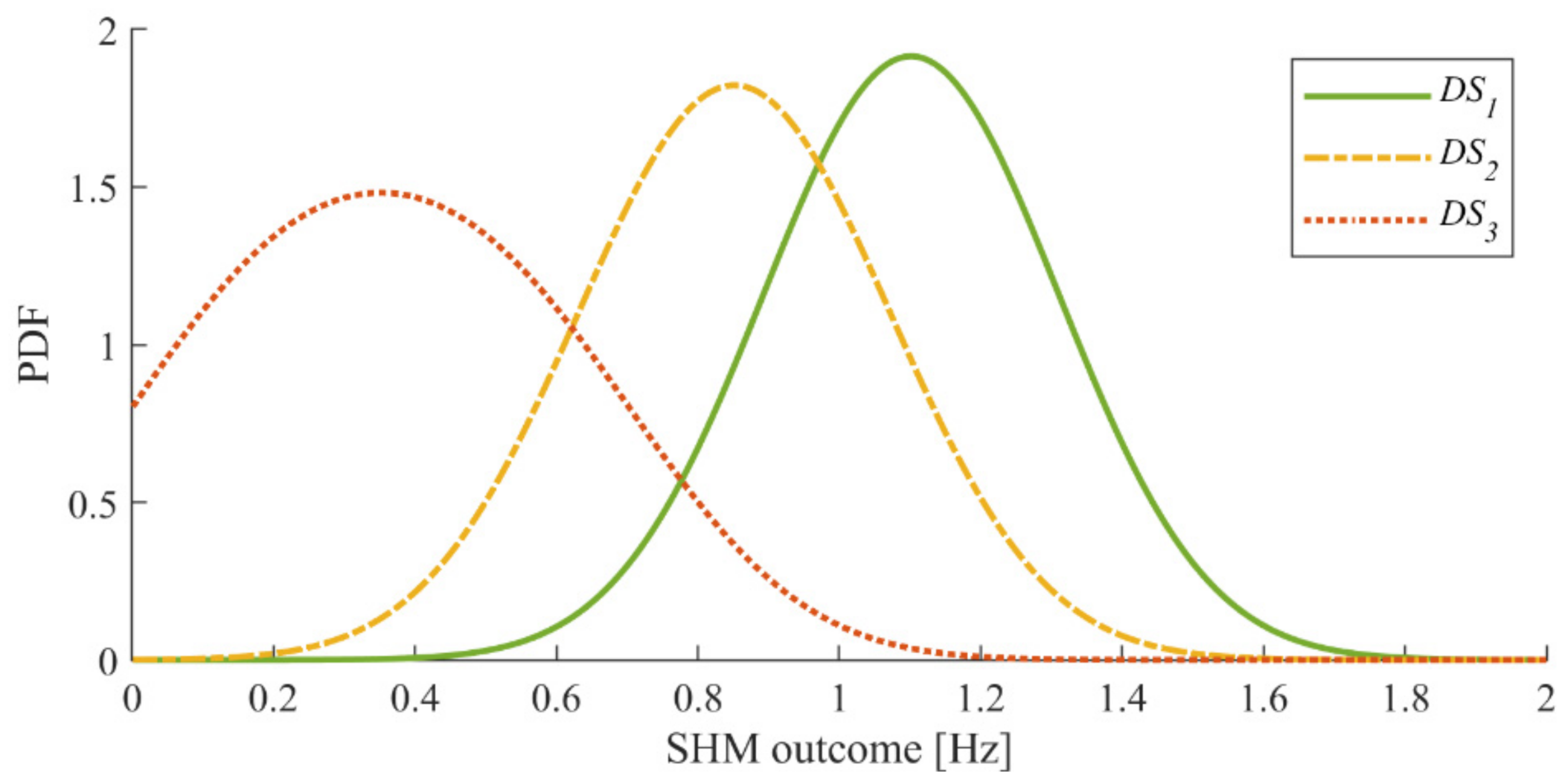
As for the distribution of the frequency values in the different states of the bridge, it is supposed that they are uniformly distributed within the corresponding frequency range. Specifically, the frequency ranges are 1.0–1.2 Hz for $D{S}_1$, 0.7–1.0 Hz for $D{S}_2$, and 0.0–0.7 Hz for $D{S}_3$. Since continuous distributions are employed, the integral version of Equation (13) is adopted. The resulting likelihood functions, shown in Figure 1, are truncated to obtain only positive frequency values.

Flood hazard. The flood hazard is modeled by exploiting a Peaks over Threshold (POT) series model [48] that is able to represent multiple flood events. First, the flood is defined as a river discharge event exceeding a flow threshold, $Q_0$. The POT model is composed of parts: (1) a probabilistic model for the annual number of events and (2) a probabilistic model for the flood intensity.

The VoI depends on $Q$, i.e., in Equation (7), $\Theta =\left[Q\right]$. The VoI for a generic flood event is obtained as follows:

$$\mathrm{VoI}={{\displaystyle \int }}_{\Theta }^{ }\mathrm{VoI}\left(\Theta \right)f\left(\Theta \right)d\Theta ={{\displaystyle \int }}_Q^{ }\mathrm{VoI}\left(Q\right)f\left(Q\right)dQ$$

(14)

The number of events in one year is assumed to follow a Poisson distribution while the flood magnitude is assumed to have a truncated exponential distribution. It is assumed that $Q_0=500 {\mathrm{m}}^3/\mathrm{s}$ and that the scale parameter of the exponential distribution of the flood magnitude is $\nu =0.0033{\left({\mathrm{m}}^3/\mathrm{s}\right)}^{-1}$.

As for the computation of the life-cycle VoI, the expected number of floods per year is 1, the reference period is 30 years, and the discount rate is 1%.

3.3. Decision Scenarios and VoI Analysis

If SHM information is not available, the management of emergencies can be carried out with a heuristic (e.g., selection of the management action based on a pre-defined system state) or with a risk-based approach (e.g., selection of the management actions that minimize the risk). The system in this case includes the bridge and the river.

In the case of flood emergency management, the heuristic approach is based on the achievement of threshold values of the demand quantified in terms of the WSEL. The risk-based approach also requires an estimation of the structural capacity (e.g., of the damage state). The latter can be supported by monitoring information that allows for a reduction of the uncertainty related to the bridge’s damage state.

In both cases, the selection of the management action can be improved by information about the system state. Such information can be relevant to the demand (water level) or the capacity (damage state).

In the following, it is assumed that the water level is known and only the value of installing an SHM system on the bridge is quantified. Two decision scenarios are considered as follows:

• Scenario 1, a risk-based decision scenario for both the Prior and the Pre-Posterior analysis;
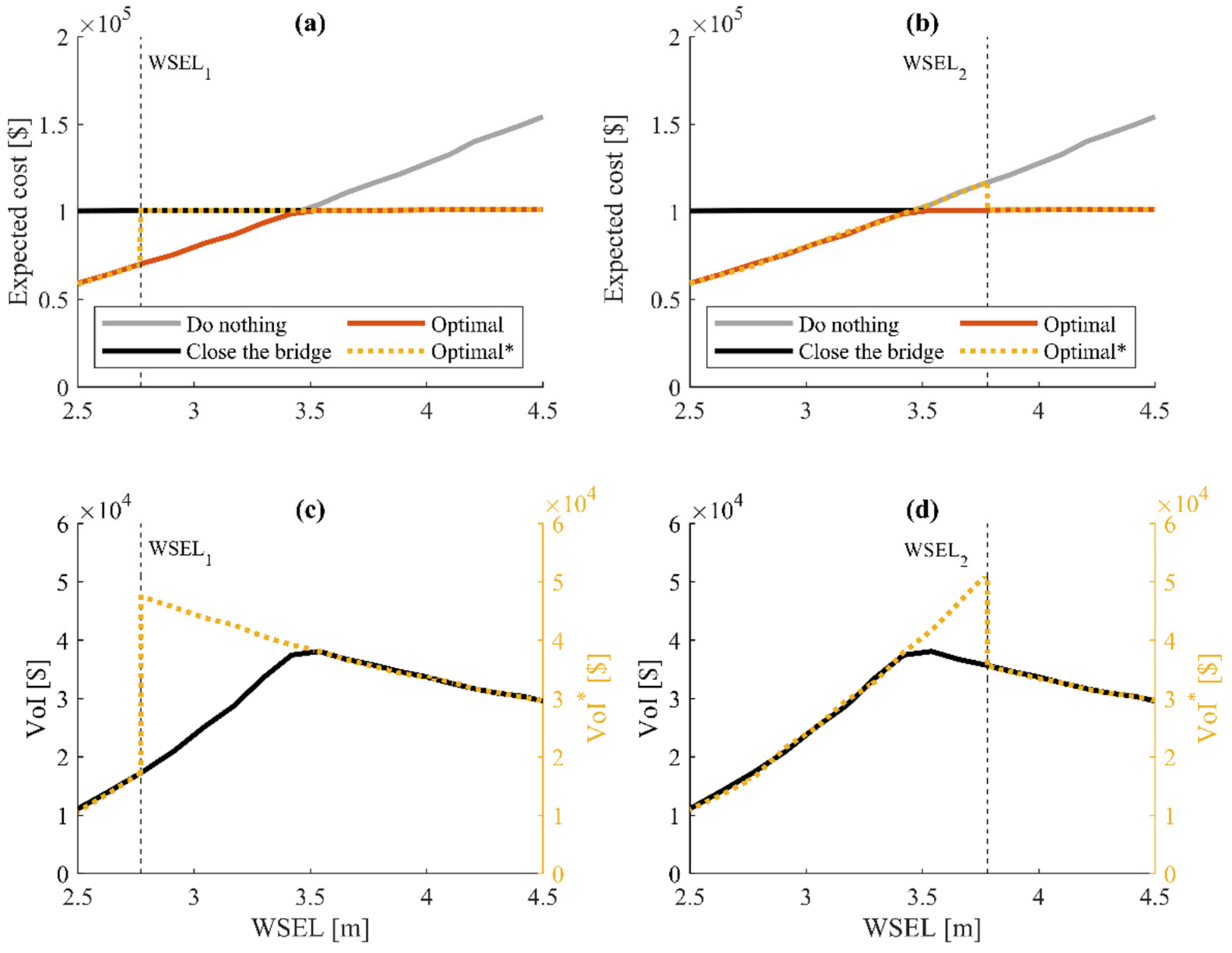
• Scenario 2, a heuristic Prior analysis and a risk-based Pre-Posterior analysis. The heuristic Prior analysis is based on the attained WSEL according to current flood emergency management procedures (see Section 3.1). Two critical WSEL thresholds are considered, i.e., WSEL₁ = 2.77 m, corresponding to Q = 600 m³/s (Scenario 2a), and WSEL₂ = 3.78 m, corresponding to Q = 1000 m³/s (Scenario 2b).

The results of the analysis are reported in Figure 2. Figure 2a,b show the results of the Prior analysis for different decision scenarios and WSEL thresholds. The grey and black solid lines display the expected costs of the actions Open and Close, respectively. The red line relates to the optimal action selected in the risk-based scenario (Scenario 1), which is the one corresponding to minimum expected costs or, equivalently, minimum risk. In this case, the critical WSEL is defined as the value of the water level for which the two actions lead to the same expected cost, i.e., roughly 3.5 m. For a WSEL lower than 3.5 m, the optimal action is Do nothing. Instead, for higher values, Close the bridge has a lower expected cost. The dotted yellow lines represent the expected cost of the optimal action in case the decision is based on the WSEL (Scenario 2). Specifically, Figure 2a shows results relating to WSEL₁ (Scenario 2a) and Figure 2b to WSEL₂ (Scenario 2b).

Figure 2c,d show the VoI as a function of the WSEL. In particular, Figure 2c refers to Scenarios 1 and 2a and Figure 2d to Scenarios 1 and 2b. The asterisk indicates that the VoI has been computed in the context of Scenario 2. Thus, it quantifies the expected reduction in management costs due to the use of both SHM information and the adoption of risk-based decision-making. For the sake of notational simplicity, in the following sections, the asterisk is specified only when needed. The VoI in the two decision scenarios is the same when the corresponding optimal prior costs coincide. In Figure 2c, this happens for WSEL < WSEL₁ = 2.77 m or WSEL > 3.5 m; in Figure 2d, this happens for WSEL < 3.5 m or WSEL > WSEL₂ = 3.78 m. For all decision scenarios, the VoI reaches the maximum in correspondence with the WSEL for which the optimal action changes, which is in the proximity of 3.5 m for Scenario 1, WSEL₁ = 2.77 m for Scenario 2a, and WSEL₂ = 3.78 m for Scenario 2b. The highest VoI peak is reached for Scenario 2b.

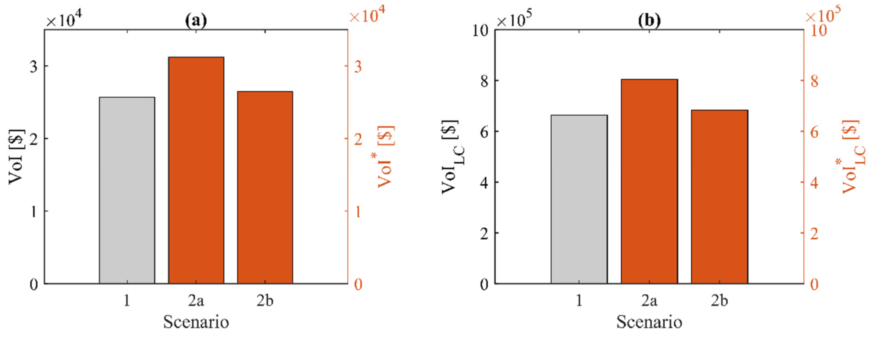
Figure 3 shows the VoI integrated over the PDF of $Q$, according to Equation (14), and the corresponding life-cycle VoI, computed according to Equation (8). In Figure 3a, the lowest VoI is associated with Scenario 1 in which risk-based decision-making is carried out during both the Prior and the Pre-Posterior analysis. In Scenario 1, the VoI as a function of the WSEL presents a value equal to or lower than the VoI obtained in Scenarios 2a and 2b. Consequently, the associated expected VoI is the lowest. The highest VoI relates to Scenario 2a, where the bridge is closed for a relatively low value of the WSEL during the Prior analysis. The intermediate VoI characterizes Scenario 2b. This can be explained by considering that even if the maximum VoI is obtained for Scenario 2b, this value is obtained for a WSEL value with a relatively low probability of occurrence (the flood magnitude is assumed to have a truncated exponential distribution, with a maximum probability density of $Q_0=500 {\mathrm{m}}^3/\mathrm{s}$). Similar considerations can be drawn for the life-cycle VoI shown in Figure 3b.

4. Post-Earthquake Emergency Management

4.1. Current Practice

Earthquakes consist of abrupt ground shaking caused by sudden movements between tectonic plates. The effects of earthquakes on transportation infrastructures depend on several factors, such as epicentral distance, soil conditions, and structural properties. Furthermore, mainshocks are generally accompanied by aftershocks which can aggravate the conditions of already damaged assets.

In the case of earthquakes, remedial actions cannot be implemented just before or during the disastrous event, as in the case of flood emergency management, but only after it has occurred. The management of bridges in the aftermath of an earthquake relates to the assessment of structural conditions, the prioritization of inspections, the definition and prioritization of interventions, and, finally, the definition of traffic limitation measures. Typically, to manage portfolios of bridges on large areas, multilevel inspections are carried out by trained technicians to assess structural conditions, restrict traffic if needed, and plan structural interventions.

As an example, a general emergency management procedure for bridges is detailed in [49]. It entails four types of inspections of increasing duration and level of detail, namely:

(i)

Fast Reconnaissance, to determine the extent of the region affected by the disastrous event;

(ii)

Preliminary Damage Assessment (PDA), to provide preliminary information on the state of each bridge and establish if further investigations are required;

(iii)

Detailed Damage Assessment (DDA), to provide detailed information about structural conditions;

(iv)

Extended investigation, to further investigate structural conditions and determine repairs or replacements.

Decisions relating to the usability of bridges, such as limiting or closing traffic, are taken after the PDA or the DDA. Specifically, after the PDA, the inspectors mark each structure as INSPECTED (good conditions—traffic allowed) or UNSAFE (uncertain or bad conditions—traffic not allowed). In case there are doubts about the structural conditions and a high consequence of failure, the structure is marked as UNSAFE and a DDA is requested. A less conservative approach is considered for lightly damaged and non-critical structures, which are marked as INSPECTED with a low-priority DDA. After the DDA, a structure is tagged as INSPECTED, LIMITED USE (uncertain conditions—only emergency vehicles allowed or heavy traffic not allowed), or UNSAFE.

In the Indiana Department of Transportation handbook [50], two types of inspections are detailed, namely:

(i)

Level 1 inspections aimed at providing a preliminary classification of structures. It comprises aerial surveys or drive-through inspections aimed at assigning a tag to each structure. The Green tag is assigned to structures in good condition, the Yellow tag to structures whose conditions are uncertain, and the Red tag to unsafe structures which should be closed to traffic.

(ii)

Level 2 inspections aimed at investigating the conditions of Yellow tagged structures in more detail. After Level 2 inspections, traffic limitations might be issued, such as restricting traffic to emergency vehicles only.

Level 1 inspections are first carried out on predetermined primary routes and on secondary routes after. During Level 2 inspection, after completing Yellow tagged bridges, Red tagged bridges are inspected to determine if they can be used with temporary repairs.

Neither in [49], nor in [50], permanent S²HM is mentioned. Instead, the assessment of bridges in the aftermath of an earthquake is generally carried out through time-consuming visual inspections. Similar procedures are also applied in the case of buildings [12].

In [51], a different decision-making approach is considered. Namely, an Aftershock Probabilistic Seismic Hazard Analysis (APSH) is first carried out to determine the residual reliability of the damaged bridge. After that, the optimal action (bridge close vs bridge open) is selected based on the comparison between the residual reliability and a given threshold: if the reliability of the bridge is lower than the threshold, the bridge is closed to traffic. To the authors’ knowledge, approaches based on residual reliability are not applied in current practice.

4.2. Case Study

The study analyzed in this section is an exemplary bridge located in a seismic area. In the aftermath of an earthquake, the decision-maker must select the optimal action between “close the bridge” and “keep the bridge open”. Before the earthquake, the decision-maker may install a vibration-based SHM system to support decision-making in case of a seismic event. Refer to [32] for a detailed description of the framework to quantify the benefit of S²HM for bridge emergency management.

Damage states. After the mainshock, the bridge can be in three damage states, namely “lightly damaged”, $D{S}_1$, “damage”, $D{S}_2$, and “severely damaged”, $D{S}_3$. The damage states are defined in terms of an Engineering Demand Parameter (EDP), such as the maximum displacement response, and EDP thresholds, $ED{P}_l$, with $ED{P}_1=$ 0. Specifically, the structure is in $D{S}_1$ for $ED{P}_1\le EDP<ED{P}_2$, in $D{S}_2$ for $ED{P}_2\le EDP<ED{P}_3$, and in $D{S}_3$ for $EDP\ge ED{P}_3$.

Prior probabilities. Prior probabilities of the damage states after a mainshock are retrieved by fragility functions expressing the probability that the EDP exceeds the thresholds $ED{P}_l$ associated with damage state $D{S}_l$ for given seismic intensity values $I_m$ as follows:

$$P\left(EDP\ge ED{P}_l\left|I_m\right.\right)=\mathsf{\Phi }\left[\frac{1}{{\beta }_{tot}}\ln \left(\frac{I_m}{I_{D{S}_l}}\right)\right]$$

(15)

where $\mathsf{\Phi }\left[·\right]$ is the standard cumulative probability function, $I_{D{S}_l}$ is the median value of the intensity measure required to cause the damage state $D{S}_l$, ${\beta }_{tot}$ is the total lognormal standard deviation, which takes into account both the uncertainty in the demand, i.e., the seismic input, and the capacity. In the absence of a more accurate estimation of ${\beta }_{tot}$, the value of 0.6 proposed by Mander [52] is used.

The intensity measure $I_m$ is obtained through the Ground Motion Prediction Equation (GMPE) proposed in [53], in the form:

$${\mathit{log}}_{10}{I}_m=\psi \left(M_m,R_m\right)+\epsilon$$

(16)

where $\psi \left(M_m,R_m\right)$ is a function that depends on $M_m$ and $R_m$ and $\epsilon$ is a random variable with a zero mean and standard deviation ${\sigma }_{\epsilon }$.

The probability that the structure is in a damage state $D{S}_l$ depends on the intensity measure of the mainshock $I_m$, and reads:

$$\left\{\begin{array}{cc}P\left(D{S}_l\left|I_m\right.\right)=P\left(EDP\ge ED{P}_l\left|I_m\right.\right)-P\left(EDP\ge ED{P}_{l+1}\left|I_m\right.\right)& for l<L\\ P\left(D{S}_l\left|I_m\right.\right)=P\left(EDP\ge ED{P}_l\left|I_m\right.\right)& for l=L\end{array}\right.$$

(17)

In this application, the Spectral Acceleration (SA) related to the fundamental period of the structure is employed as an intensity measure. Since $P\left(EDP\ge ED{P}_1\left|I_m\right.\right)=1$ and three damage states have been introduced, two fragility functions must be defined. The following $I_{D{S}_l}$ values are assumed in this application: $I_{D{S}_2}=1 {\mathrm{m}/\mathrm{s}}^2$ and $I_{D{S}_3}=1.5 {\mathrm{m}/\mathrm{s}}^2$.

Probabilities of failure. It is assumed that aftershocks are the leading cause of structural failure in the aftermath of the mainshock. The probability of failure due to aftershocks depends on the damage state of the structure after the mainshock and on the characteristics of the mainshock itself, as well as the considered duration of the aftershock sequence.

The probability of failure due to the occurrence of an aftershock of intensity $I_a$ can be quantified through aftershock fragility functions which express the probability of structural failure for a bridge already in $D{S}_l$ as follows:

$$P\left(F\left|I_a,D{S}_l\right.\right)=\mathsf{\Phi }\left[\frac{1}{{\beta }_{tot}}\ln \left(\frac{I_a}{I_{F\left(D{S}_l\right)}}\right)\right]$$

(18)

where $I_{F\left(D{S}_l\right)}$ is the median intensity measure of the aftershock required to cause the structure in $D{S}_l$ to fail. The intensity measure $I_a$ is obtained through the GMPE used for $I_m$. The following $I_F{}_{D{S}_l}$ values are assumed in this application: $I_{F\left(D{S}_1\right)}=3.0 {\mathrm{m}/\mathrm{s}}^2$, $I_{F\left(D{S}_2\right)}=2.50 {\mathrm{m}/\mathrm{s}}^2$, and $I_{F\left(D{S}_3\right)}=2.00 {\mathrm{m}/\mathrm{s}}^2$.

The intensity of the aftershocks is not known in advance. Therefore, the probability distribution of $I_a$ should be considered to quantify the probability of failure due to a generic aftershock, $P^{\ast }\left(F\left|M_m,R_m,D{S}_l\right.\right)$, as follows:

$$P^{\ast }\left(F\left|M_m,R_m,D{S}_l\right.\right)={{\displaystyle \int }}_{I_a}P\left(F\left|I_a,D{S}_l\right.\right)f\left(I_a\left|M_m,R_m\right.\right)d{I}_a$$

(19)

where $f\left(I_a\left|M_m,R_m\right.\right)$ is the PDF of $I_a$, which, generally, is conditional on the magnitude of the earthquake $M_m$ and the epicentral distance from the bridge $R_m$.

After the mainshock, in a period [t; t+T], more than one aftershock may occur. Assuming the aftershock sequence as a Poisson process, the probability of failure in [t; t+T] can be approximated to:

$$P\left(F|\Phi \right)=P\left(F\left|M_m\right.,R_m,D{S}_l,t,T\right)=1-e^{-N_F\left(M_m,R_{m}D{S}_l,t,T\right)}$$

(20)

where $\Phi =\left[M_m,R_m,D{S}_l,t,T\right]$ and $N_F\left(M_m,R_{m}D{S}_l,t,T\right)$ is the expected number of aftershocks leading to structural failure in [t; t+T]. $N_F$ can be estimated as follows:

$$N_F\left(M_m,R_m,D{S}_l,t,T\right)=P^{\ast }\left(F\left|M_m,R_m,D{S}_l\right.\right)N_a\left(M_m,t,T\right)$$

(21)

where $N_a\left(M_m,t,T\right)$ is the expected number of aftershocks in [t; t+T].

Costs. To facilitate the comparison of results, the costs of bridge failure and survival used for the previous case study (displayed in Table 3) are considered.

Likelihood functions. An S²HM system that provides the first natural frequency of the bridge is considered. This parameter is expected to decrease in the presence of damage, such as the formation of plastic hinges due to seismic actions. As for the costs, to simplify the comparison of results, the likelihood functions adopted for the previous case study (shown in Figure 1) are employed.

Seismic hazard. The quantification of the VoI in seismic emergency management requires mainshock and aftershock hazard models. As for the mainshock, the PDF of $M_m$ is modeled as a truncated exponential function [23] as follows:

$$f\left(M_m\right)=\frac{\beta e^{-\beta M_m}}{e^{-\beta M_{m,l}}-e^{-\beta M_{m,u}}}$$

(22)

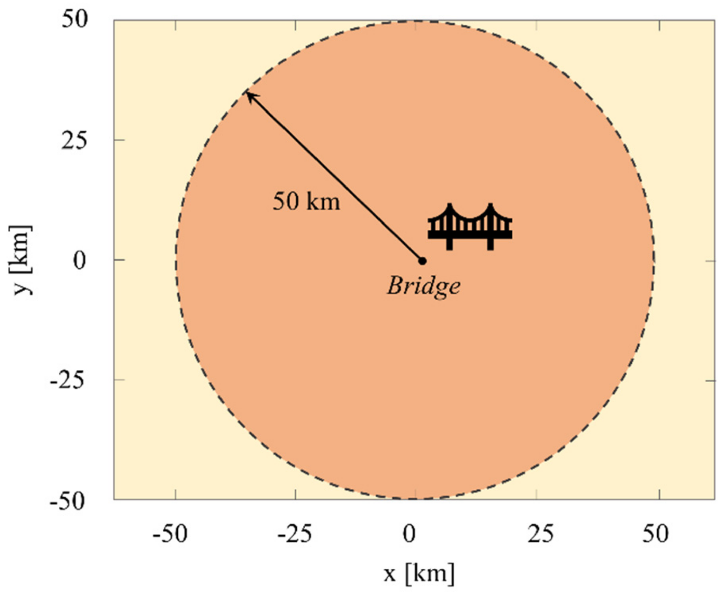
where $M_{m,l}$ and $M_{m,u}$ are the lower and upper bounds, respectively, of the mainshock magnitude and $\beta =bln10$, where b is the Negative slope of the Gutenberg−Richter law. Mainshocks are supposed to be generated with uniform probability in any location of the circular seismogenic area shown in Figure 4.

Aftershocks are modeled as a non-homogeneous Poisson process. Under the assumption that the upper magnitude bound for aftershocks is equal to the magnitude of the mainshock that has generated them, the PDF of $M_a$ reads:

$$f\left(M_a\left|M_m\right.\right)=\frac{\beta e^{-\beta \left(M_a-M_{m,l}\right)}}{1-e^{-\beta \left(M_m-M_{m,l}\right)}}$$

(23)

The mean number of aftershocks in the period [t; t+T] following a mainshock of magnitude $M_m$ is computed as follows:

$$N_a\left(M_m,t,T\right)=\frac{{10}^{a+b\left(M_m-M_{m,l}\right)}-{10}^a}{p-1}\left[{\left(c+t\right)}^{1-p}-{\left(c+t+T\right)}^{1-p}\right]$$

(24)

where a, b, c, and p are parameters characteristic of the seismic area. Aftershocks are supposed to occur with uniform probability in a circular region centered at the epicenter of the mainshock [54]. The area of this region is a function of the intensity of the mainshock [55], namely:

$$S_a={10}^{M_m-4.1}$$

(25)

Aftershock locations have uniform probability inside this area and zero probability outside. Given the above considerations, the PDF of $I_a$ can be expressed as follows:

$$f\left(I_a\left|M_m,R_m\right.\right)={{\displaystyle \iint }}_{M_a,R_a}f\left(I_a\left|M_a,R_a\right.\right)f\left(M_a\left|M_m\right.\right)f\left(R_a\left|M_m,R_m\right.\right)d{M}_{a}d{R}_a$$

(26)

The parameters characterizing mainshocks and aftershocks are displayed in

Table 4. Mainshock and aftershock parameters.

Mainshock		Aftershock
Variable	Value	Variable	Value
$\mathrm{Minimum} \mathrm{magnitude}, M_{m,l}$	5	$a$	−1.71
$\mathrm{Maximum} \mathrm{magnitude}, M_{m,u}$	9	$b$	0.97
$\mathrm{Negative} \mathrm{slope}, b$	1	$\mathit{log}c$	−1.46
		$p$	0.94

. The duration of the emergency phase is assumed to be two weeks after the mainshock, i.e., $t=0$ and $T=14 \mathrm{days}$.

According to the definition of the seismic hazard, the VoI not only depends on $I_m$, but also on $M_m$ and $R_m$, i.e., $\Theta =\left[M_m,R_m,I_m\right]$. The VoI for a generic mainshock reads:

$$\begin{array}{c}\mathrm{VoI}={{\displaystyle \int }}_{\Theta }^{ }\mathrm{VoI}\left(\Theta \right)f\left(\Theta \right)d\Theta =\hfill \\ ={\int \int \int }_{M_m,R_m,I_m}\mathrm{VoI}\left(M_m,R_m,I_m\right)f\left(I_m\left|M_m,R_m\right.\right)f\left(M_m\right)f\left(R_m\right)d{I}_{m}d{M}_{m}d{R}_m\hfill \end{array}$$

(27)

Regarding the computation of the life-cycle VoI, the expected number of mainshocks per year $\lambda$ is 0.1, the reference period is 30 years, and the discount rate is 1%.

4.3. VoI Analysis

In the case of seismic emergency management, the S²HM system can provide information on both the seismic action and the state of the bridge after the mainshock. In turn, this information reduces the uncertainty in both the seismic demand and the structural capacity and supports risk-based decision-making. In this application, it is supposed that the S²HM system provides information only on the structural condition. Specifically, the VoI is quantified considering two decision scenarios, namely:

• Scenario 1, a risk-based decision scenario for both the Prior and the Pre-Posterior analysis;
• Scenario 2, a heuristic Prior analysis and risk-based Pre-Posterior analysis. The heuristic Prior analysis is based on the prior knowledge of the decision-maker on the state of the bridge, which, for instance, comes from an expeditious visual inspection. Two situations are analyzed: first, the bridge is closed because it is not considered safe, without risk considerations (Scenario 2a); second, the bridge is not closed because it is considered safe or deeper investigations are planned (Scenario 2b).

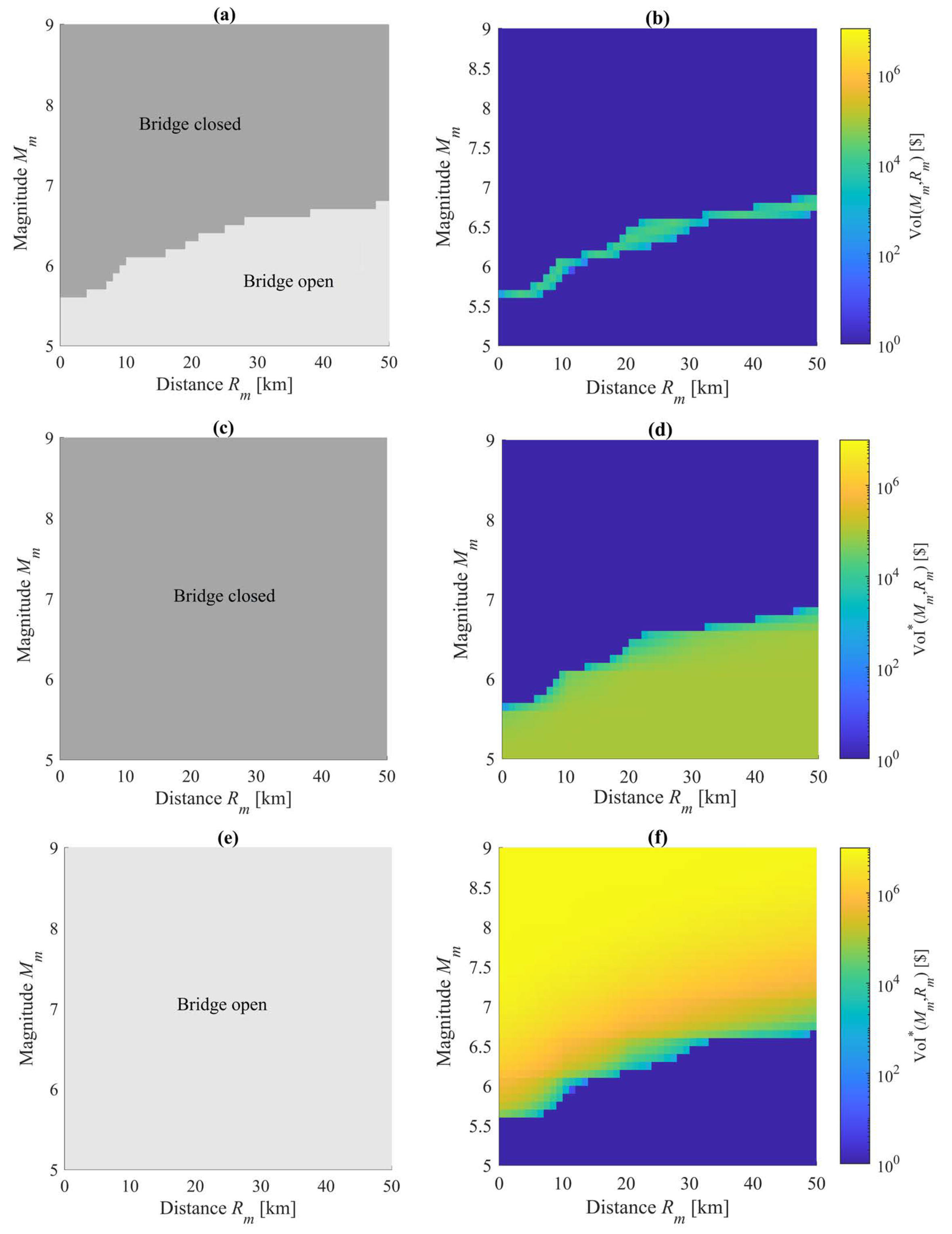
The results of the VoI analysis for different decision scenarios are shown in Figure 5. In particular, Figure 5a displays the results of the Prior analysis according to risk considerations, i.e., the optimal action is the one corresponding to minimum expected costs (minimum risk) according to the epicentral distance and magnitude of the mainshock (Scenario 1). The bridge should be closed for a mainshock of relatively high magnitude and/or short epicentral distance (north-left corner). Otherwise, it should not be closed to traffic (south-right corner). The corresponding VoI is shown in Figure 5b. The VoI is at the maximum in correspondence with the boundary between the optimal actions in Figure 5a, which is when the two actions have similar expected costs during the Prior analysis.

Figure 5c relates to Scenario 2a, which is when the bridge is closed because it is not considered safe (without performing in-depth analyses). Again, the asterisk is associated with Scenario 2 and indicates that the VoI is generated by the SHM information and the adoption of risk-based decision-making. The associated value of SHM information is displayed in Figure 5d. The VoI is particularly high in the south-right corner, which is approximately where the optimal action is leaving the bridge open according to the risk-based Prior analysis (see Figure 5a). In this case, the SHM information may indicate that the bridge is in good condition, thus it should not be closed. In turn, the VoI is high because the SHM information might lead the decision-maker to select a different optimal action with respect to the Prior analysis (when the optimal action was always closing the bridge). Instead, in the north-right corner, the VoI is null. Here, the SHM information indicates that the bridge is in bad condition. Thus, it does not modify the choice of the optimal action and the resulting VoI is null.

Figure 5e relates to Scenario 2b, i.e., when the bridge is not closed using prior information. The corresponding VoI shown in Figure 5f is particularly high in the north-left corner, which roughly corresponds to the area in Figure 5a where the optimal action is closing the bridge. In this situation, the S²HM information may suggest that the bridge is in bad condition. Thus, the decision-maker might select to close the bridge to traffic. The VoI in Figure 5f reaches higher values than the VoI shown in Figure 5d. According to Table 3, the cost of failure when the bridge is open is higher than the other costs. Thus, considering the costs at stake, leaving the bridge open when it should be closed generates higher costs than closing the bridge when it could be left open.

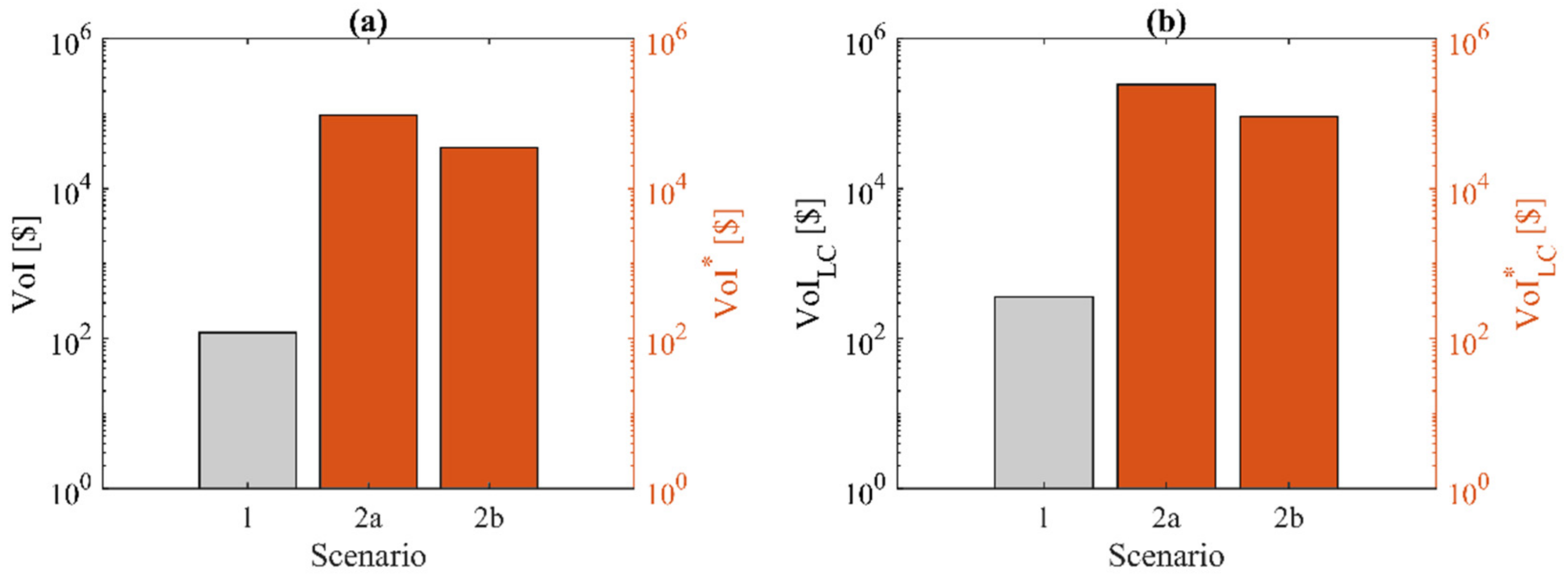
Figure 6 shows the VoI and the life-cycle VoI computed considering the parameters specified in Section 4.2. In Figure 6a, the lowest VoI is quantified for Scenario 1, due to the relatively small conditional VoI displayed in Figure 5b. Even if the highest values of the conditional VoI are reached in Scenario 2b (see Figure 5f), the highest expected VoI is obtained for Scenario 2a. This is due to the PDF of the $M_m$ and $R_m$. For instance, $M_m$ presents a truncated exponential distribution, which associates high probabilities to small values of magnitude. In turn, in Scenario 2a, low magnitudes are linked to relatively high values of the VoI. In Scenario 2b, low magnitudes are linked to null values of the VoI. Thereby, the expected VoI is higher in the case of Scenario 2a. The life-cycle VoI values shown in Figure 6b for the three scenarios are similar to the corresponding VoI values due to the low expected number of earthquakes in one year in the seismic area ($\lambda =0.1$).

5. Discussion

In the previous sections, two case studies on the emergency management of bridges are analyzed in the case of floods or seismic events, respectively. For each type of hazard, a framework for computing the value of SHM (or S²HM) information in emergency management is described and applied considering reference bridges. To facilitate the comparison of results, similar case studies are considered. Specifically, the management actions, the number of damage states, the costs of failure and survival, and the likelihood functions are the same in the two cases. Probabilities of failure and hazard modeling are tailored to the specific case. For each case study, three decision scenarios are considered, involving different Prior analyses made with different assumptions, and the same Pre-Posterior analysis is made according to the Bayesian decision theory, i.e., according to risk considerations. The rationale is that SHM can potentially provide real-time information about structural conditions and thus support risk-based decision-making.

In Scenario 1, decision-making is made according to risk considerations during both the Prior and the Pre-Posterior analysis. This Prior scenario is generally not realistic, since, in practice, during the Prior analysis—without SHM information—decision-makers base their actions on engineering judgment or heuristic methods. Scenarios 2a involve conservative Prior emergency decision-making where the bridge is closed for a relatively low value of the WSEL in case of flood or closed as a precaution after a seismic event. In turn, Scenarios 2b involve non-conservative Prior emergency decision-making where the bridge is closed only for a relatively high value of the WSEL in case of flood or not closed at all after a seismic event. In brief, the Prior analyses in Scenarios 2a and 2b entail suboptimal actions from the point of view of the Bayesian decision theory.

For both case studies, the VoI computed in Scenario 1 is lower than the ${\mathrm{VoI}}^{\ast }$ computed in Scenario 2a or 2b. The VoI computed in Scenario 1 quantifies the expected reduction in management costs obtained when both the Prior and the Pre-Posterior analyses are carried out selecting the actions which minimize the expected costs. Instead, the VoI* computed in Scenario 2 is obtained also considering non-optimal actions during the Prior analysis, which, in turn, are associated with higher expected costs. For this reason, the VoI* is always higher or equal to the VoI. The difference between the two quantities is not due to the SHM information but to the different decision-making approach, i.e., risk-based instead of heuristic decision-making.

The maximum values of the conditional ${\mathrm{VoI}}^{\ast }$ are reached for Scenarios 2a (see Figure 2 and Figure 5). Leaving the bridges open (when they could be in a bad health state) might result in high direct and indirect costs in case of failure. In this dangerous condition, the SHM information is particularly valuable since it might give insight into the actual structural conditions and lead the decision-maker to change their actions. Nevertheless, in both cases, the maximum expected ${\mathrm{VoI}}^{\ast }$ is obtained for Scenarios 2b. This is due to the probabilistic models used to represent $Q$ and the couple $\left(M_m,R_m\right)$ that assign higher probabilities of occurrence to low-intensity events, which, in turn, are associated with a higher ${\mathrm{VoI}}^{\ast }$ in Scenarios 2b.

The VoI and the life-cycle VoI for the three decision scenarios present similar values in the case of flood management (roughly in the range $6–8·{10}^5$). Instead, in the case of a seismic event, they differ by several orders of magnitude (roughly in the range (${10}^2$–${10}^6$). This is because suboptimal actions are selected in the Prior analysis for a large set of couples $\left(M_m,R_m\right)$ (see Figure 5). On the contrary, in the case of flood management, suboptimal actions only relate to a small set of $Q$ values (see Figure 2).

6. Conclusions

This paper investigates the VoI from SHM in the case of the emergency management of bridges. The VoI is quantified in the realm of the Bayesian decision theory, which bases the selection of the optimal action on the principle of maximum utility. In engineering contexts, this is equivalent to selecting the action associated with minimal risk. Nevertheless, emergency management in real practice is generally based on engineering judgment or heuristic methods in cases where an SHM is not installed. In turn, the availability of real-time SHM information can potentially support risk-based decision-making and, ultimately, optimize the management of infrastructures.

The impact of the decision scenario on the VoI is investigated considering different types of prior decision scenarios—in which the SHM information is not available—and a risk-based pre-posterior scenario—which is carried out before the collection of SHM information, simulating that it is available. Two case studies relating to the emergency management of bridges under flood and seismic hazards are considered. The general framework for computing the VoI in emergency management is reported and then tailored to the two types of hazards. The limitations of the analysis are similar to those of any other VoI analysis and relate to the difficulties of determining all the required ingredients, such as likelihood functions, fragility functions, hazard models, probabilities of failure, and costs. Despite the VoI depending on the specific case study, some general findings can be drawn. Specifically, it has been demonstrated that the decision scenarios underlying the VoI analysis must be carefully evaluated. Considering non-realistic prior decision scenarios can lead to underestimating the benefit of SHM and risk-based decision-making in emergency management. Instead, in these situations, SHM might provide valuable information to decision-makers and prevent the selection of suboptimal emergency management actions. The reduction in expected management costs resulting from the Pre-Posterior analysis is not only determined by the use of SHM information but also by the adoption of risk-based decision-making.

Future works will address different types of decision scenarios, such as decision-making under reliability constraints, as well as more realistic case studies.

References

- Bocchini, P.; Frangopol, D.M. Optimal Resilience- and Cost-Based Postdisaster Intervention Prioritization for Bridges along a Highway Segment. J. Bridge Eng. 2012, 17, 117–129. [Google Scholar] [CrossRef]
- Zhong, J.; Gardoni, P.; Rosowsky, D. Seismic fragility estimates for corroding reinforced concrete bridges. Struct. Infrastruct. Eng. 2012, 8, 55–69. [Google Scholar] [CrossRef]
- Ganesh Prasad, G.; Banerjee, S. The Impact of Flood-Induced Scour on Seismic Fragility Characteristics of Bridges. J. Earthq. Eng. 2013, 17, 803–828. [Google Scholar] [CrossRef]
- Dueñas-Osorio, L.; Craig, J.I.; Goodno, B.J. Seismic response of critical interdependent networks. Earthq. Eng. Struct. Dyn. 2007, 36, 285–306. [Google Scholar] [CrossRef]
- Hammond, M.J.; Chen, A.S.; Djordjević, S.; Butler, D.; Mark, O. Urban flood impact assessment: A state-of-the-art review. Urban Water J. 2015, 12, 14–29. [Google Scholar] [CrossRef] [Green Version]
- Zhang, G.; Liu, Y.; Liu, J.; Lan, S.; Yang, J. Causes and statistical characteristics of bridge failures: A review. J. Traffic Transp. Eng. 2022, 9, 388–406. [Google Scholar] [CrossRef]
- Wardhana, K.; Hadipriono, F.C. Analysis of Recent Bridge Failures in the United States. J. Perform. Constr. Facil. 2003, 17, 144–151. [Google Scholar] [CrossRef] [Green Version]
- Montalvo, C.; Cook, W.; Keeney, T. Retrospective Analysis of Hydraulic Bridge Collapse. J. Perform. Constr. Facil. 2020, 34, 04019111. [Google Scholar] [CrossRef]
- Flora, A.; Cardone, D.; Vona, M.; Perrone, G. A simplified approach for the seismic loss assessment of rc buildings at urban scale: The case study of Potenza (Italy). Buildings 2021, 11, 142. [Google Scholar] [CrossRef]
- Han, R.; Li, Y.; van de Lindt, J. Seismic Loss Estimation with Consideration of Aftershock Hazard and Post-Quake Decisions. ASCE-ASME J. Risk Uncertain. Eng. Syst. Part A Civ. Eng. 2016, 2, 04016005. [Google Scholar] [CrossRef]
- Kilanitis, I.; Sextos, A. Impact of earthquake-induced bridge damage and time evolving traffic demand on the road network resilience. J. Traffic Transp. Eng. 2019, 6, 35–48. [Google Scholar] [CrossRef]
- Cardone, D.; Flora, A.; De Luca Picione, M.; Martoccia, A. Estimating direct and indirect losses due to earthquake damage in residential RC buildings. Soil Dyn. Earthq. Eng. 2019, 126, 105801. [Google Scholar] [CrossRef]
- Quqa, S.; Landi, L.; Diotallevi, P.P. Seismic structural health monitoring using the modal assurance distribution. Earthq. Eng. Struct. Dyn. 2021, 50, 2379–2397. [Google Scholar] [CrossRef]
- Limongelli, M.P.; Çelebi, M. Seismic Structural Health Monitoring; Springer International Publishing: Cham, Switzerland, 2019. [Google Scholar] [CrossRef]
- Rainieri, C.; Notarangelo, M.A.; Fabbrocino, G. Experiences of Dynamic Identification and Monitoring of Bridges in Serviceability Conditions and after Hazardous Events. Infrastructures 2020, 5, 86. [Google Scholar] [CrossRef]
- Dolce, M.; Nicoletti, M.; De Sortis, A.; Marchesini, S.; Spina, D.; Talanas, F. Osservatorio sismico delle strutture: The Italian structural seismic monitoring network. Bull. Earthq. Eng. 2017, 15, 621–641. [Google Scholar] [CrossRef] [Green Version]
- Prendergast, L.J.; Gavin, K. A review of bridge scour monitoring techniques. J. Rock Mech. Geotech. Eng. 2014, 6, 138–149. [Google Scholar] [CrossRef]
- Lin, Y.-B.; Chen, J.-C.; Chang, K.-C.; Chern, J.-C.; Lai, J.-S. Real-time monitoring of local scour by using fiber Bragg grating sensors. Smart Mater. Struct. 2005, 14, 664–670. [Google Scholar] [CrossRef]
- Maroni, A.; Tubaldi, E.; Ferguson, N.; Tarantino, A.; McDonald, H.; Zonta, D. Electromagnetic Sensors for Underwater Scour Monitoring. Sensors 2020, 20, 4096. [Google Scholar] [CrossRef]
- Malekjafarian, A.; Kim, C.; Obrien, E.J.; Prendergast, L.J.; Fitzgerald, P.C.; Nakajima, S. Experimental demonstration of a mode shape-based scour monitoring method for multi-span bridges with shallow foundations. J. Bridge Eng. 2020; in press. [Google Scholar] [CrossRef]
- Rainieri, C.A.; Gargaro, D.A.; Fabbrocino, G.I.; Maddaloni, G.; Di Sarno, L.; Prota, A.N.; Manfredi, G. Shaking table tests for the experimental verification of the effectiveness of an automated modal parameter monitoring system for existing bridges in seismic areas. Struct. Control Health Monit. 2018, 25, e2165. [Google Scholar] [CrossRef]
- Zhang, W.-H.; Lu, D.-G.; Qin, J.; Thöns, S.; Faber, M.H. Value of information analysis in civil and infrastructure engineering: A review. J. Infrastruct. Preserv. Resil. 2021, 2, 16. [Google Scholar] [CrossRef]
- Thöns, S. On the Value of Monitoring Information for the Structural Integrity and Risk Management. Comput. Civ. Infrastruct. Eng. 2018, 33, 79–94. [Google Scholar] [CrossRef]
- Straub, D. Value of information analysis with structural reliability methods. Struct. Saf. 2014, 49, 75–85. [Google Scholar] [CrossRef]
- Pozzi, M.; Der Kiureghian, A. Assessing the value of information for long-term structural health monitoring. In Health Monitoring of Structural and Biological Systems; Kundu, T., Ed.; SPIE Press: San Diego, CA, USA, 2011; p. 79842W. [Google Scholar] [CrossRef]
- Giordano, P.F.; Quqa, S.; Limongelli, M.P. The value of monitoring a structural health monitoring system. Struct. Saf. 2023, 100, 102280. [Google Scholar] [CrossRef]
- Malings, C.; Pozzi, M. Conditional entropy and value of information metrics for optimal sensing in infrastructure systems. Struct. Saf. 2016, 60, 77–90. [Google Scholar] [CrossRef]
- Kamariotis, A.; Chatzi, E.; Straub, D. A framework for quantifying the value of vibration-based structural health monitoring. Mech. Syst. Signal. Process 2023, 184, 109708. [Google Scholar] [CrossRef]
- Giordano, P.F.; Iacovino, C.; Quqa, S.; Limongelli, M.P. The value of seismic structural health monitoring for post-earthquake building evacuation. Bull. Earthq. Eng. 2022, 20, 4367–4393. [Google Scholar] [CrossRef]
- Faber, M.H. Statistics and Probability Theory. In Pursuit of Engineering Decision Support; Springer Netherlands: Dordrecht, The Netherlands, 2012. [Google Scholar] [CrossRef]
- Raiffa, H.; Schlaifer, R. Applied Statistical Decision Theory. Boston: Division of Research; Graduate School of Business Administration, Harvard University: Boston, MA, USA, 1961. [Google Scholar]
- Giordano, P.F.; Limongelli, M.P. The value of structural health monitoring in seismic emergency management of bridges. Struct. Infrastruct. Eng. 2020, 18, 537–553. [Google Scholar] [CrossRef]
- Giordano, P.F.; Prendergast, L.J.; Limongelli, M.P. Quantifying the value of SHM information for bridges under flood-induced scour. Struct. Infrastruct. Eng. 2022. [Google Scholar] [CrossRef]
- Zonta, D.; Glisic, B.; Adriaenssens, S. Value of information: Impact of monitoring on decision-making. Struct. Control Health Monit. 2014, 21, 1043–1056. [Google Scholar] [CrossRef]
- Tubaldi, E.; White, C.J.; Patelli, E.; Mitoulis, S.A.; De Almeida, G.; Brown, J.; Cranston, M.; Hardman, M.; Koursari, E.; Lamb, R.; et al. Invited perspectives: Challenges and future directions in improving bridge flood resilience. Nat. Hazards Earth Syst. Sci. 2022, 22, 795–812. [Google Scholar] [CrossRef]
- Tubaldi, E.; Maroni, A.; McDonald, H.; Zonta, D. Monitoring-Based Decision Support System for Risk Management of Bridge Scour, Proceedings of the 1st Conference of the European Association on Quality Control of Bridges and Structures. EUROSTRUCT 2021, Padua, Italy, 29 August–1 September 2021; Lecture Notes in Civil Engineering; Springer: Cham, Switzerland, 2022; Volume 200, pp. 877–884. [Google Scholar] [CrossRef]
- Crotti, G.; Cigada, A. Scour at river bridge piers: Real-time vulnerability assessment through the continuous monitoring of a bridge over the river Po, Italy. J. Civ. Struct. Health Monit. 2019, 9, 513–528. [Google Scholar] [CrossRef]
- Ayres Associates. FIELD MANUAL. Scour Critical Bridges: High-Flow Monitoring and Emergency Procedures; Idaho Department of Transportation: Boise, Idaho, 2004. [Google Scholar]
- CAE. Roads at Risk of Flooding? Sardinia Invests in Technology and Safety. 2020. Available online: https://www.cae.it/eng/news/roads-at-risk-of-flooding-sardinia-invests-in-technology-and-safety.-nw-1364.html (accessed on 1 November 2022).
- Giordano, P.F.; Prendergast, L.J.; Limongelli, M.P. The value of different monitoring systems in the management of scoured bridges. In Experimental Vibration Analysis for Civil Engineering Structures; Springer: Cham, Switzerland, 2023. [Google Scholar] [CrossRef]
- National Academies of Sciences, Engineering, and Medicine. Risk-Based Management Guidelines for Scour at Bridges with Unknown Foundations; The National Academies Press: Washington, DC, USA, 2007. [Google Scholar] [CrossRef]
- Johnson, P.A.; Clopper, P.E.; Zevenbergen, L.W.; Lagasse, P.F. Quantifying Uncertainty and Reliability in Bridge Scour Estimations. J. Hydraul. Eng. 2015, 141, 04015013. [Google Scholar] [CrossRef]
- Davis, D.W.; Burnham, M.W. Accuracy of Computed Water Surface Profiles; Hydraulic Engineering; U.S. Army Corps of Engineers: Washington, DC, USA, 1987; pp. 818–823.
- Johnson, P.A.; Dock, D.A. Probabilistic bridge scour estimates. J. Hydraul. Eng. 1998, 124, 750–754. [Google Scholar] [CrossRef]
- Ghosn, M.; Moses, F.; Wang, J. Design of Highway Bridges for Extreme Events; Transportation Research Board: Washington, DC, USA, 2003. [Google Scholar]
- Caspani, V.F.; Tonelli, D.; Poli, F.; Zonta, D. Designing a Structural Health Monitoring System Accounting for Temperature Compensation. Infrastructures 2021, 7, 5. [Google Scholar] [CrossRef]
- Kamariotis, A.; Chatzi, E.; Straub, D. Value of information from vibration-based structural health monitoring extracted via Bayesian model updating. Mech. Syst. Signal Process. 2022, 166, 108465. [Google Scholar] [CrossRef]
- Kottegoda, N.T.; Rosso, R. Applied Statistics for Civil and Environmental Engineers; Wiley-Blackwell: Hoboken, NJ, USA, 2009. [Google Scholar]
- National Academies of Sciences, Engineering, and Medicine. Assessing, Coding, and Marking of Highway Structures in Emergency Situations—Volume 3: Coding and Marking Guidelines; The National Academies Press: Washington, DC, USA, 2016. [Google Scholar] [CrossRef]
- Ramirez, J.A.; Frosch, R.J.; Sozen, M.A.; Turk, A.M. Handbook for the Post-Earthquake Evaluation of Bridges and Roads; Indiana Department of Transportation: Indianapolis, IN, USA, 2000. [Google Scholar]
- Alessandri, S.; Giannini, R.; Paolacci, F. Aftershock risk assessment and the decision to open traffic on bridges. Earthq. Eng. Struct. Dyn. 2013, 42, 2255–2275. [Google Scholar] [CrossRef]
- Mander, J. Fragility Curve Development for Assessing the Seismic Vulnerability of Highway Bridges; Technical Report, MCEER HighwayProject; FHWA: Philadelphia, PA, USA, 1999. [Google Scholar]
- Bindi, D.; Pacor, F.; Luzi, L.; Puglia, R.; Massa, M.; Ameri, G.; Paolucci, R. Ground motion prediction equations derived from the Italian strong motion database. Bull. Earthq. Eng. 2011, 9, 1899–1920. [Google Scholar] [CrossRef] [Green Version]
- Iervolino, I.; Chioccarelli, E.; Giorgio, M. Aftershocks’ Effect on Structural Design Actions in Italy. Bull. Seismol. Soc. Am. 2018, 108, 2209–2220. [Google Scholar] [CrossRef]
- Utsu, T. Aftershocks and Earthquake Statistics(1): Some Parameters Which Characterize an Aftershock Sequence and Their Interrelations. J. Fac. Sci. Hokkaido Univ. 1970, 3, 129–195. [Google Scholar]
Figure 1.
Likelihood functions for scoured foundations.
Figure 2.
Flood emergency management. Results of the VoI analysis as a function of the WSEL for different decision scenarios: (a) Results of the Prior analysis for Scenarios 1 and 2a; (b) Results of the Prior analysis for Scenarios 1 and 2b; (c) VoI for Scenarios 1 and 2a; (d) VoI for Scenarios 1 and 2b.
Figure 3.
Flood emergency management: (a) VoI and (b) VoILC for different decision scenarios.
Figure 4.
Bridge and seismogenic area.
Figure 5.
Post-earthquake emergency management. Results of the VoI analysis as a function of and for different decision scenarios: (a) Results of the Prior analysis for Scenario 1; (b) VoI for Scenario 1; (c) Results of the Prior analysis for Scenario 2a; (d) VoI for Scenario 2a; (e) Results of the Prior analysis for Scenario 2b; (f) VoI for Scenario 2b.
Figure 6.
Post-earthquake emergency management: (a) VoI and (b) VoILC for different decision scenarios (on a logarithmic scale).