Enriching Roadside Safety Assessments Using LiDAR Technology: Disaggregate Collision-Level Data Fusion and Analysis

Abstract

Fatalities and serious injuries still represent a significant portion of run-off-the-road (ROR) collisions on highways in North America. In order to address this issue and design safer and more forgiving roadside areas, more empirical evidence is required to understand the association between roadside elements and safety. The inability to gather that evidence has been attributed in many cases to limitations in data collection and data fusion capabilities. To help overcome such issues, this paper proposes using LiDAR datasets to extract the information required to analyze factors contributing to the severity of ROR collisions on a localized collision level. Specifically, the paper proposes a new method for extracting pole-like objects and tree canopies. Information about other roadside assets, including signposts, alignment attributes, and side slopes is also extracted from the LiDAR scans in a fully automated manner. The extracted information is then attached to individual collisions to perform a localized assessment. Logistic regression is then used to explore links between the extracted features and the severity of fixed-object collisions. The analysis is conducted on 80 km of roads from 10 different highways in Alberta, Canada. The results show that roadside attributes vary significantly for the different collisions along the 80 km analyzed, indicating the importance of utilizing LiDAR to extract such features on a disaggregate collision level. The regression results show that the steepness of side slopes and the offset of roadside objects had the most significant impacts on the severity of fixed-object collisions.

1. Introduction

Run-off-the-road (ROR) collisions account for a third of serious collisions on rural roads [1,2]. The reason these collisions often result in serious injuries or fatalities is that a large portion of them end in vehicles either overturning or colliding at high speeds with fixed objects. In fact, statistics show that fixed-object collisions represented 30.3% of the fatal collisions and 17.7% of serious injury collisions on US highways in 2016 [3].

In attempts to mitigate the severity of ROR collisions, there have been attempts to make the roadside environment more forgiving. This includes having traversable clear zones where the roadside area is clear of any hazards and where side slopes are recoverable [4]. Such practice maximizes the chance of recovery for errant vehicles. Although some roadside objects could be removed to clear up the roadside area, other objects such as luminaire support poles and structures supporting high load powerlines are challenging to relocate. In fact, luminaire poles actually have important positive impacts on safety due to their role in reducing nighttime collisions [5,6]. As a result, design guides including AASHTO and the Transportation Association of Canada’s (TAC) design guide recommend that, if objects were to be placed in the clear zone, these objects are shielded to provide sufficient protection to drivers. Furthermore, in cases where clear zone requirements cannot be met, design guides recommend providing sufficient lateral offset.

Despite the importance of the information included in roadside design guides, some of it was added several decades ago. For instance, information in the AASHTO’s design guide on clear zones has not changed since 1977. Furthermore, a significant portion of this information is based on qualitative measures and best practices as opposed to actual relationships between substantive safety measures and roadside hazards [7,8]. When referring to recommendations on clear zone design, the AASHTO guide acknowledges that the recommendations “… are based on limited empirical data that were extrapolated to provide information for a wide range of conditions” [4]. One challenge to updating design guides with more recent information is limited data collection capabilities. Manual collection of all the relevant roadside assets, including side slopes, poles, and trees, to analyze the relationships between these assets and the severity of fixed-object collisions is a tedious process. Lee and Mannering [9] describe this as a “chronic lack of data” that has represented an obstacle to the development of statistical models relating roadside features to collision frequency and severity. As a result, most analysis in this area has been limited to information extracted from police reports of varying reliability.

One technology that has been extremely valuable in this regard due to its ability to produce highly detailed maps of road infrastructure is mobile Light Detection and Ranging (LiDAR) technology. LiDAR datasets consist of closely spaced points that form an accurate 3D model of a highway. Unlike static laser scanning and other conventional surveying methods, a Mobile Laser Scanner (MLS) can collect data while traveling at highway speeds. This makes detailed maps of road infrastructure readily available to transportation agencies with minimal effort. Research has shown that, if properly utilized, LiDAR datasets could be used for the extraction of multiple features, including signposts, roadside poles, trees, and many other elements of roadside infrastructure [10,11,12,13,14].

Our paper contributes to the existing literature in three different areas. Firstly, we propose a new method for the segmentation of pole-like objects and tree canopies from LiDAR. The method involves voxelizing the point cloud to isolate non-ground objects. A longitudinal analysis of point spread is then conducted to distinguish poles from the tree canopy.

Secondly, our paper demonstrates the feasibility of utilizing mobile LiDAR datasets when conducting advanced roadside safety assessments. Besides poles and tree canopy, our assessment involves automated extraction of other roadside features (e.g., traffic signs and sideslope information) on 80 km of collision-prone highways. We adopt a localized approach for feature extraction whereby roadside features within the local vicinity of every collision recorded on the analyzed highway segments were extracted automatically. It is worth noting here that even in situations where such extractions are performed from LiDAR using off-the-shelf products, this is conducted manually and involves hours of user interaction.

Finally, our paper explores potential links between extracted features and the severity of fixed-object ROR collisions along with the analyzed segments. The paper extracts roadside information specifically for a selection of collision-prone segments considered in the assessment, as opposed to selecting the road segments based on data availability.

2. Literature Review

2.1. Pole-Like Object Extraction from LiDAR

Several different studies have attempted extracting roadside assets and design elements from mobile LiDAR data [15,16,17,18,19,20,21]. This includes multiple attempts that focused on the extraction of pole-like objects [22,23]. Yang and Dong [24] employed a radius search group of neighboring points within the point cloud. The authors then used a supervised classification method to classify the points into linear, planar, and spherical points based on local geometric features. Lehtomäki et al. [25] proposed a scanline-based algorithm to extract pole-like objects from mobile LiDAR data. Poles sweeps within scanlines were detected, and longitudinal clustering was employed to combine different pole layers. Clusters that constitute the same pole were merged using principal component analysis (PCA).

Pu et al. [26] employed a surface growing algorithm to remove ground surface and then assessed different quartiles to detect poles. El-Halawany and Lichti [27] used DBSCAN to detect high-density clusters in local neighborhoods with a radius of 25 cm. Vertical region growing was then used to extract upright objects. Object height range, the normal surface direction, Yan et al. [28], and the largest normalized eigenvalue were then used to classify the upright objects and proposed a four-step procedure to extract poles and towers from LiDAR. The method involved ground filtering using a statistical skewness balancing algorithm, unsupervised clustering using DBSCAN, and classification based on a set of geometric decision rules.

In more recent work [12,29,30,31], multiple voxel-based methods, where the point cloud is converted into a 3D grid before processing, were proposed. The subsequent processing pipeline varied between the papers and included plane filtering, region growing, a combination of supervised and unsupervised classification, and clustering.

Li and Cheng [32] employed super voxels over-segmentation followed by region growing to detect the vertical component of pole-like objects. Other parts of the pole were then detected using uphill clustering, and spatial correspondence between the vertical poles and their attachments were analyzed to combine different elements of the pole-like object. The authors reported a recall of 92.4%.

Although many methods were developed to extract pole-like objects from LiDAR, the majority of those methods were developed for urban environments where distinguishing between tree canopy cover and pole-like objects was not critical. To address this gap, the method proposed in this paper introduces a lateral layer-based assessment to distinguish poles and tree canopy. The method also differs from previous techniques in that the ground-non-ground segmentation also is also voxel-based, reducing the need for additional processing.

2.2. Data Sources in Previous Roadside Safety Assessments

Several studies have analyzed the relationship between roadside assets and collision frequency or severity, each utilizing data from different sources. In an early study, Jones and Baum [33] used data in police reports from 1975 to analyze the impact of factors including speeds, grades, pole density, and pole offset on the likelihood of a single-vehicle (SV) collision involving pole contact. They found that poles were the objects most frequently struck in SV collisions and that pole density and pole offset had the most significant effects on the severity of pole collisions.

Fox, Good, and Joubert [34] conducted site visits to locations where collisions had occurred to collect site characteristics. Among other variables, the authors analyzed the impacts of pole offset on the likelihood of pole-related collisions. The study found that when offset was minimized to 0 m (i.e., the pole was placed on the edge of the road), the likelihood of a pole-related collision was 3.5 times as high when compared to an offset of 3 m. This led the authors to conclude that poles must be placed at least 3 m away from the edge of the road. Max and Mason [35] combined data from police reports with data collected in site visits to analyze the impact of utility poles on collisions. The authors also found that pole-related collisions were overrepresented at offsets of 3 m or less from the edge of the road.

In a comprehensive earlier study, Zegeer and Parker, Jr. [36] used several statistical techniques to model utility pole collisions. The authors extracted most variables, including pole offset information and pole positions from photologs. For some variables, trained technicians had to inspect the photos and estimate the information, while for others, such as pole offset, distances were obtained by using a calibrated grid placed over the photolog viewing screen. The authors found that lateral pole offset, pole density, and road slopes were primary geometric factors related to utility pole collision frequency. The study also found that utility pole collisions decreased significantly as pole offsets and pole densities increased.

Good, Fox, and Joubert [37] used data collected from tow-truck operators and site visits from a research team to analyze factors impacting utility pole collisions. The authors reported similar findings in terms of greater pole offset leading to a reduction in utility pole collisions. Furthermore, the authors also found that the relative risk of utility pole collisions increased dramatically for pole offsets under 3 m. No additional decrease in relative risk was found for pole offsets of greater than 3 m.

Lee and Mannering [9] combined data collected in GPS surveys with information extracted from the Washington State database to investigate the effects of fixed objects on ROR collisions. The authors developed a zero-inflated negative binomial model to assess the impacts of roadside features on collision frequency and a multinomial logit model to assess collision severity. The authors found that increasing light pole offset and reducing the density of isolated trees helped decrease the frequency of ROR collisions. It was also found that multiple roadside features, including poles and slopes, contributed to increasing the severity of ROR collisions.

Holdridge, Shankar, and Ulfarsson [38] used information in Washington State police reports to develop multivariate nested logit models to analyze the relationships between roadside objects and the severity of fixed-object collisions. Large wooden poles, including utility poles and trees, were found to increase the likelihood of fatal injuries. Schneider, Savolainen, and Zimmerman [39] also developed a multinomial logit model to assess the impacts of roadside objects on ROR collision severity. Trees were found to be the highest contributor to incapacitating and fatal injuries in ROR collisions, although most other roadside objects were also associated with significant increases in injury severity.

El Esawey and Sayed [7] used data from BC Collision Information System (CIS) and developed safety performance functions to analyze the relationship between pole placement and density and pole collision frequency. The authors found that increasing the offset of poles and decreasing their density both had positive impacts on safety. In addition, increasing pole offset was reported to have more significant impacts on reducing collision frequency than reducing pole density.

Xie, Zhao, and Huynh [40] utilized a latent class logit model to analyze injury severity in SV collisions on rural roads. The data were acquired from the Florida Traffic Crash Database, and the results showed that trees, utility poles, and concrete barriers were all contributing factors to the severity of SV ROR collisions. Park and Abdel-Aty [41] combined data from Florida DOTs Roadway Characteristic Inventory and Crash Analysis Reporting System databases to assess the impacts of several roadside treatments on safety. The authors found that increasing the offset of poles and trees resulted in a reduction in collision frequency.

Roque, Moura, and Cardoso [42] utilized data from the police force, Guarda Nacional Republicana, to develop multinomial and mixed logit models and analyze the impacts of unforgiving roadside areas on the severity of ROR collisions in Portugal. The authors found that critical slopes were high contributors to fatalities.

In summary, most previous studies were limited to information in police reports site visits when collecting data for the analysis of fixed-object collisions. Although one study used photologs for some feature extraction, those photologs were manually inspected. Accordingly, most studies in this area have been limited by extremely tedious and error-prone data collection techniques. Furthermore, many studies performed the assessment on an aggregate level where the roadside attributes of the entire segment are considered as opposed to information in the vicinity of the collision. This paper aims to demonstrate the feasibility of overcoming such challenges by utilizing mobile LiDAR technology and automatically extracting roadside information.

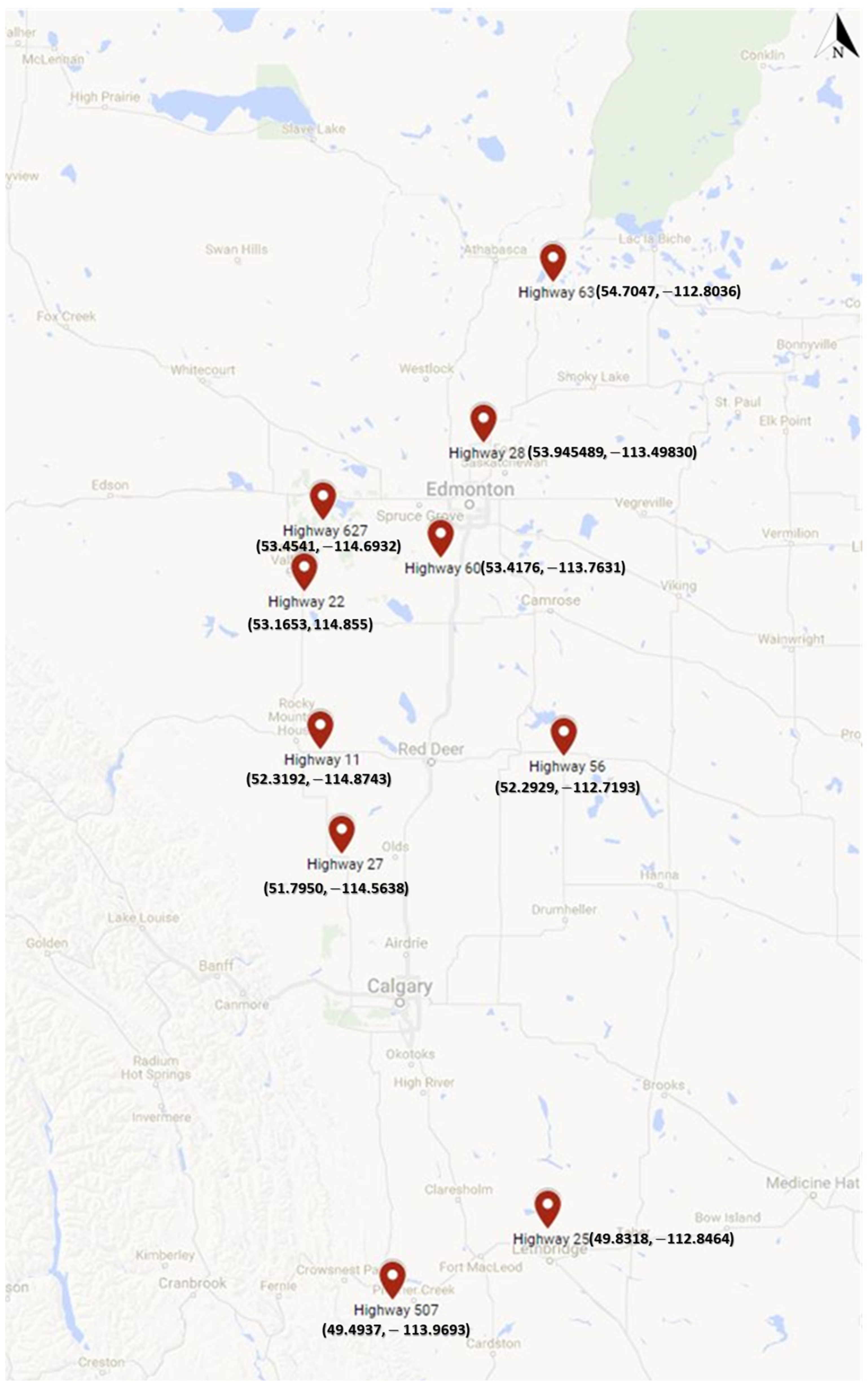
3. Data Collection and Test Segments

Data considered in this study included the LiDAR scans and collision information. LiDAR data were collected by Alberta Transportation (AT) in surveys conducted on multiple highways across the province. In mobile laser scanning (MLS), a vehicle mounted with a scanning system travels highway corridors at highway speeds to collect data. The product is a 360° representation of the road’s environment. The MLS system used in this study is the RIEGL VMX-450, which is equipped with two VQ-450 scanners as well as an Inertial Measurement Unit and a Global Navigation Satellite System. The VQ-450 scanner has a scan rate of up to 1.1 million points per second and a scan speed of 400 lines per second, a precision of 5 mm, and an accuracy of 8 mm [43].

Collision data were extracted from the AT collision database for the period (2009–2014). The database includes information about collision severity (Fatal, Injury, PDO), the collision location (highway control segment and coordinates), and the type of collision (fixed-object ROR, in case of this paper).

Analysis was conducted on a set of collision-prone highways distributed among different parts of Alberta (see Figure 1). All segments considered in this paper were identified as collision-prone segments in an Empirical Bayes (EB) assessment of 17,355 two-way-two-lane segments in Alberta by Tawfeek and El-Basyouny [44]. The EB method is considered the most consistent collision-prone identification method and provides the most reliable results when compared to the other methods [45]. In total 80-km of roads from 10 different crash-prone highways were considered in the analysis. On those segments, 100 fixed-object collisions were recorded in the analysis period.

The next section includes a detailed description of the algorithms that were developed and used to automatically extract roadside features from the LiDAR scans.

4. Methodology

The analysis in this paper was split into 2 different phases. Phase I involved the extraction of roadside objects from the LiDAR datasets. In Phase II, logistic regression was used to explore the relationships between the severity of fixed-object ROR collisions and roadside characteristics.

4.1. Feature Extraction

Although LiDAR scans create a highly detailed representation of the roadside area, the size and the unorganized nature of those datasets make efficiently extracting information from them a highly challenging and time-consuming process. To overcome such challenges, Phase I of this work focused on the development and employment of fully automated algorithms to extract features of interest. Features considered in this study included the density of roadside objects and their offsets, horizontal alignment information, and side slopes steepness. The remainder of this section includes details of the feature extraction methods. Before discussing the details of the extraction algorithms, it is worth noting that the computational requirements for running the extraction algorithms are relatively low. All the extraction algorithms were run on an Intel i7 CPU with 16 GB of RAM.

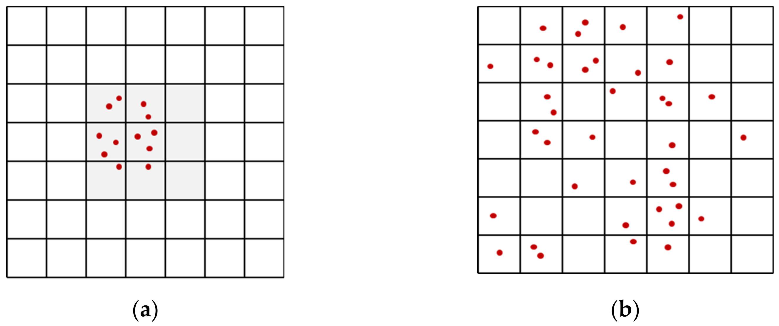
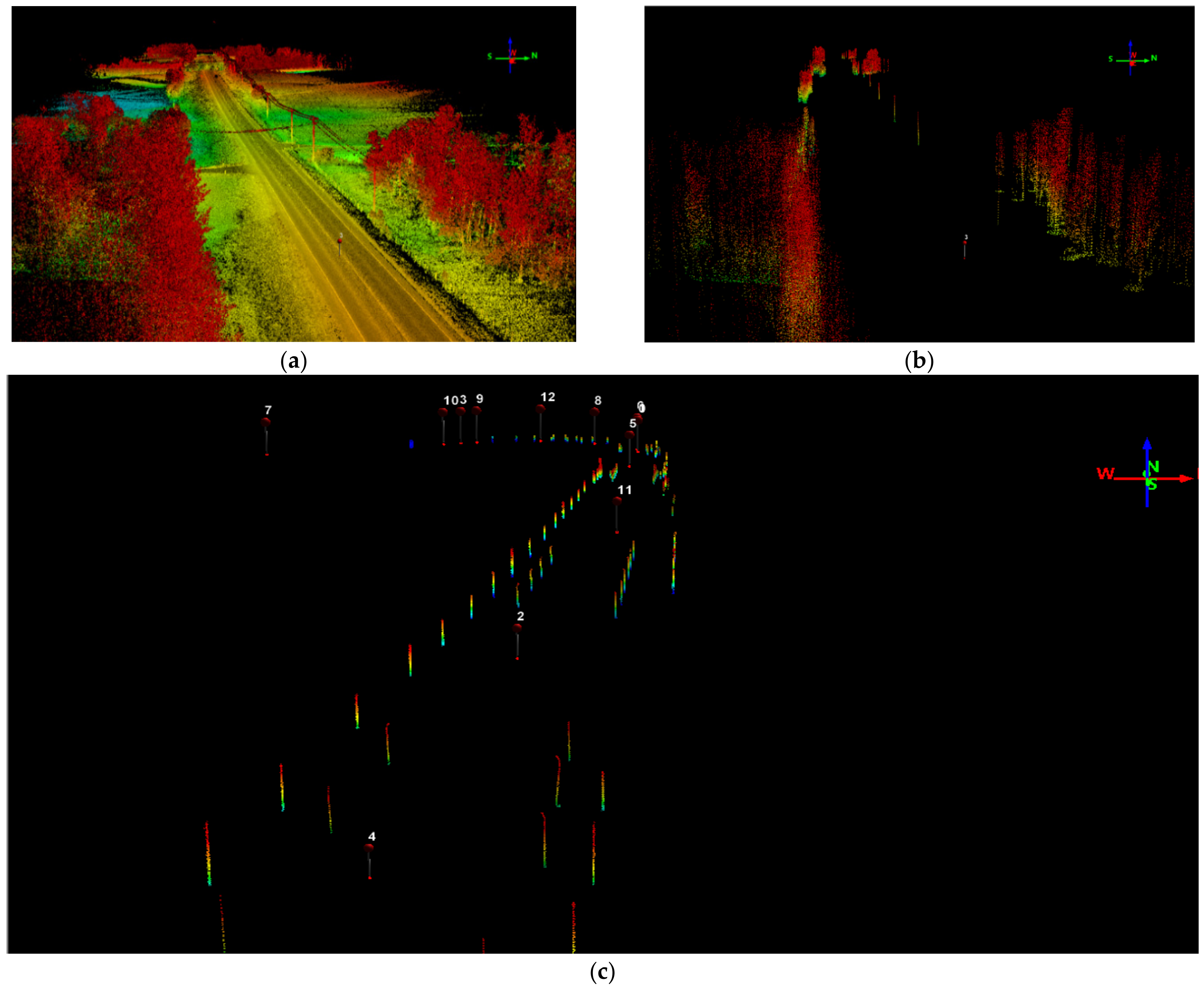
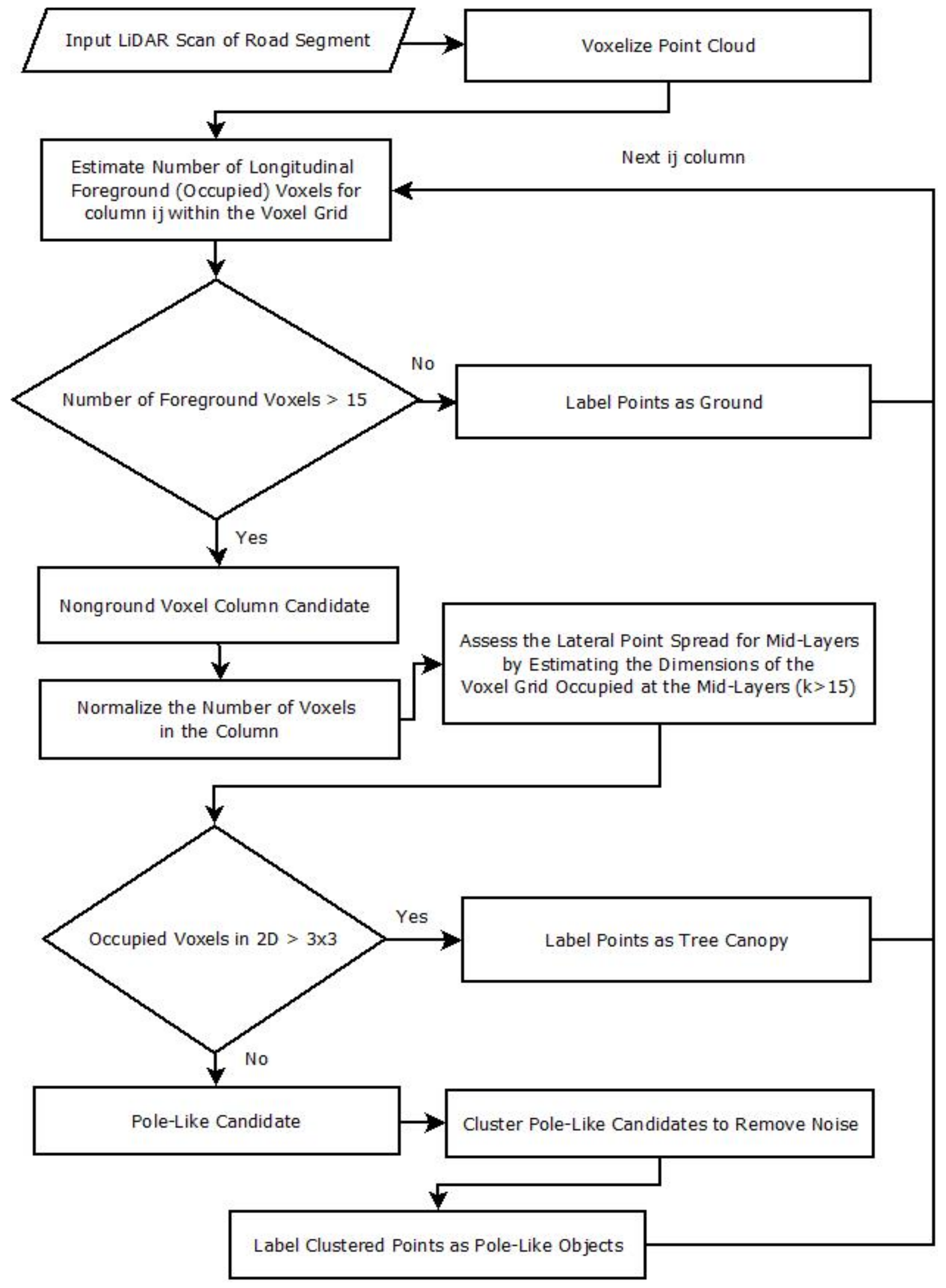
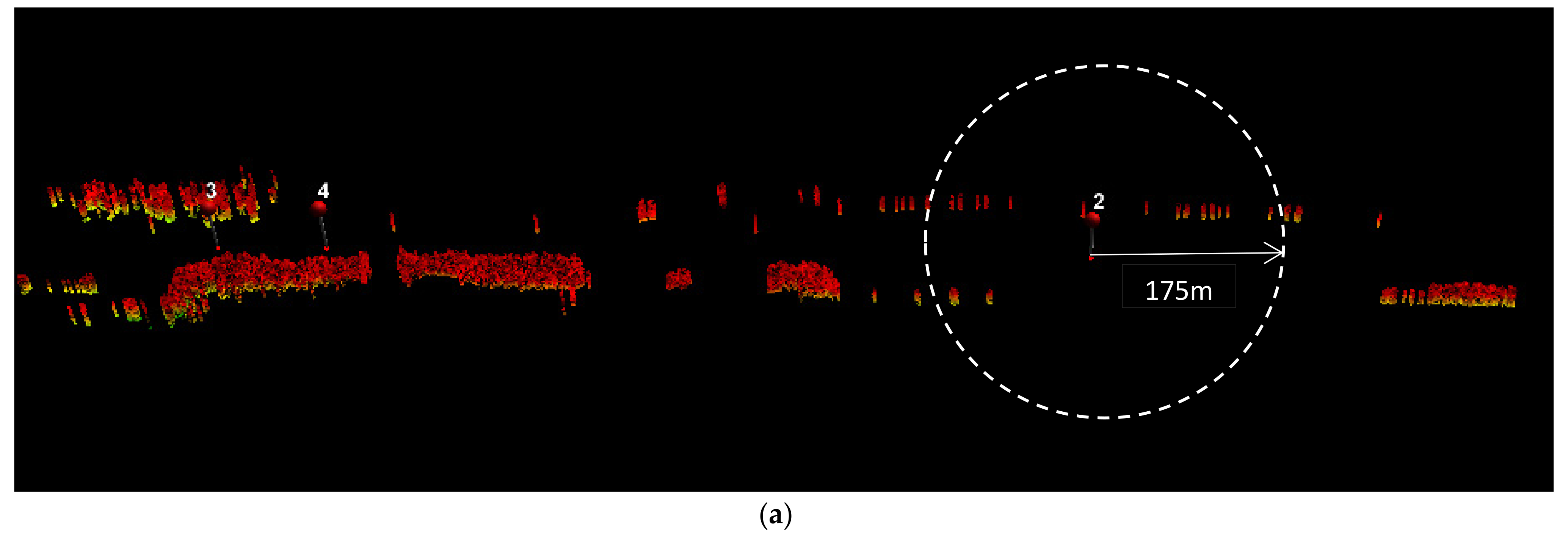
4.1.1. Pole-Like Object Extraction

The first step of the pole extraction involves voxelizing the data into 3D voxels of 0.4 m. A 0.4 m voxel size ensures that the majority of pole-like objects would fall in a single voxel or at least in 3 × 3 neighborhood of voxels. Assuming v(i, j, k) denotes a voxel and v(I, J, k) denotes all voxels in layer k. If V represents the voxel grid system consisting of K layers, then the V can be defined as the union of all voxel layers:

$$V={\displaystyle \underset{k=0}{\overset{K}{{\displaystyle \mathsf{\cup }}}}}k$$

(1)

A point P(x, y z) is assigned to a voxel v(i, j, k) as follows. If Δx, Δy, and Δz denote the dimensions of a single cell (v) in the x, y, and z directions and x_o, y_o, and z_o denote the origin of the voxel grid (V), then the ID of the voxel, v(i, j, k), in which the point P(x, y, z) falls can be computed as follows:

$$i=\frac{int\left(x-x_o\right)}{{\Delta }_x}$$

(2)

$$j=\frac{int\left(y-y_o\right)}{{\Delta }_y}$$

(3)

$$k=\frac{int\left(z-z_o\right)}{{\Delta }_z}$$

(4)

After voxelization, a search for stacks of foreground (occupied) voxels in z was conducted. A minimum threshold of 15 foreground voxels was specified as a cut-off point for a stack of voxels to be considered as one where a pole-like object potentially exists. A 15-voxel threshold was used because the Alberta Highway Lighting Guide specifies the standard luminaire mounting height for pole placement as 6.0 m, which translates to 15 voxels [46].

Since the 15-voxel cut-off was the minimum threshold, the number of foreground voxels for all pole-like objects detected was not the same. Hence, the next step was to normalize the number of vertical layers for all non-ground objects. This was conducted by splitting all non-ground objects into 10 layers of fixed height.

After extracting the non-ground objects, they were classified into pole-like objects and objects that belonged to a group of trees (i.e., tree canopy), which was conducted in multiple stages. Stage 1 involved analyzing point spread in the mid-layers of the extracted non-ground object with the aims of isolating pole-like objects and isolated trees from tree canopy. It is expected that with pole-like objects, such as utility poles and isolated trees (i.e., trees that are not part of a canopy and stand-alone without any neighboring vegetation, see Figure 2 left), points would spread no more than a single voxel in each direction of the xy plane from the centroid of the object (see Figure 3). Therefore, it was assumed that if all points belonging to the object at the mid-layer occupied a 3 × 3 voxel grid (i.e., 1.2 m × 1.2 m) in the xy-plane, then it was highly likely that this object was an isolated pole-like object, such as those in Figure 3a and Figure 4c. In contrast, if there was a spread of points beyond the 3 × 3 grid then the object was classified as either a pole-like object with noise or a tree belonging to a forest canopy.

Stage 2 involved distinguishing between pole-like objects with noise and tree canopy. To achieve this, the lateral point density was analyzed across multiple vertical layers along with the height of the non-ground object. If the spread was consistent across multiple layers and occupied a 2D area of more than 3 × 3 voxels, then it was highly likely that the object was part of a forest canopy seen in Figure 3b. All other objects that did not meet this criterion were classified as potential pole-like objects with noise or other non-ground objects (e.g., building facades… etc.).

Stage 3 involved removing noise from pole-like objects with noise. To achieve this noisy pole-like objects were clustered using DBSCAN, which is a Density-Based Clustering algorithm for Applications with Noise. Here, if more than 2 neighboring objects were clustered into a single cluster, these objects were considered large objects (e.g., building facades) and were not considered as poles anymore. In contrast, if points surrounding the pole-like object were eliminated by the algorithm, they were noise points.

DBSCAN was also used to group trees within close proximity. A hit count of 4 and $\epsilon$ = 30 m were used for clustering since it is highly unlikely for any object that has a lower hit count (number of points) and higher voxel spacing to be part of the same tree canopy.

A sample of the extracted pole-like objects is shown in Figure 4c. Figure 5 shows a summary of the segmentation steps.

Table 1. Result validity assessment.

Metric 1	Results on AB-20-02
Precision (%)	98
Recall (Detection Rate) (%)	79

¹ For information on how the metrics were computed see [12].

shows the validity metrics computed after testing the algorithm on a 4 km segment of AB-20-02. To collect ground truth information for the evaluation, the number of pole-like objects along the were manually counted using google satellite imagery and the LiDAR scan. The algorithm was then used to extract pole-like objects from the LiDAR scan of segment, and the results were compared to the manual extraction. It is worth noting that the highway 20 test segment was not used in developing the segmentation criteria it was only used for validation. The recall was estimated at 79% with a precision of 98% on this segment, which was an improvement on the results obtained by [12] after testing on the same segment.

4.1.2. Side Slope Estimation

Side slopes were also extracted at locations where collisions had occurred. The algorithm proposed by Gargoum [47] was used to estimate side slopes. The method is fully automated and involves (i) extracting cross-sections along the highway, (ii) identifying the edges of the cross-sections, and (iii) estimating the cross and side slopes.

The algorithm first estimates the trajectory vectors parallel to the road’s axis by finding the difference between position vectors. Let $\widehat{P}$₁ be the position vector defining the start-point of the trajectory vector. Similarly, let $\widehat{P}$₂ represent the position vector representing the end-point of the trajectory vector. In that case, the trajectory vector (${\widehat{V}}_i$) at a point i along the road can be defined as follows:

$${\widehat{V}}_i={\widehat{P}}_2-{\widehat{P}}_1$$

(5)

where, ${\widehat{P}}_1=\left[\begin{array}{c}{x}_1\\ y_1\\ z_1\end{array}\right]$ and ${\widehat{P}}_2=\left[\begin{array}{c}{x}_2\\ y_2\\ z_2\end{array}\right]$, hence ${\widehat{V}}_i$ can be rewritten as follows:

$${\widehat{V}}_i=\left[\begin{array}{c}{x}_2\\ y_2\\ z_2\end{array}\right]-\left[\begin{array}{c}{x}_1\\ y_1\\ z_1\end{array}\right]=\left[\begin{array}{c}{x}_2-x_1\\ y_2-y_1\\ z_2-z_1\end{array}\right]$$

(6)

The normal vector (Ni) a vector normal to the trajectory vector (Vi) was then estimated, as follows

$$N_i=\left[\begin{array}{ccc}{v}_y& -v_x& v_z\end{array}\right]$$

(7)

where, v_x, v_y, and v_z are the components of the trajectory vector (Vi).

Points within close proximity of the plane parallel to Ni are then retained and extracted, representing the cross-section. Once the cross-section was extracted and rotated, the extents of the cross-sections side slopes were defined, and the slope was estimated. Readers interested in more detailed information about the procedure are referred to [47].

4.1.3. Traffic Sign Post Extraction

Sign panel reflectivity was used to distinguish traffic signs from other pole-like objects. The method used for sign extraction was a fully automated algorithm proposed by Gargoum et al. [48]. The method involved (i) intensity filtering (extracting points with high reflectivity), (ii) density-based clustering, (iii) buffer-zone filtering (based on position from the road’s edge), and (iv) geometric filtering. Readers interested in details of the procedure are referred to [48].

4.1.4. Curve Detection and Radii Estimation

Other variables extracted from the LiDAR data included (i) the existence of a horizontal curve on a crash site and (ii) the radius of the horizontal curve. Horizontal curve information was extracted based on the algorithm proposed by Gargoum et al. [49]. The method involved (i) trajectory vector definition (similar to that discussed as part of the side slope estimation in Equations (5) and (6)), (ii) azimuth-based curve detection (where changes in azimuth were analyzed to detect the endpoints of horizontal curves), (iii) curve radius estimation, which was achieved by first locating the origin of the curve through the intersection of the lines normal to the two tangents, then estimating the distance between PC, PT, and the origin. Readers interested in details of the procedure are referred to [49]. It is worth noting that other features could also have been extracted from the point clouds including passing and stopping sight distance [50].

4.2. Logistic Regression

Since only 3 levels of severity (PDO, Injury, and Fatal) are coded into Alberta collision data, and due to the limited number of fatal collisions, severity was coded as a binary variable where a collision was either severe (1) or non-severe (0). Logistic regression was used to analyze the effects of attributes of the road infrastructure on the severity of fixed-object ROR collisions. Binary Logistic Regression is a form of logistic regression where the dependent variable (DV) is a binary categorical variable that can belong to one of two levels. The impacts of several independent variables on the DV are then estimated.

Let $Y_i$ be the dependent variable that denotes the severity of collision i. In this case, $p_i=P\left(Y_i=k\right)$ represents the probability of collision i belonging to severity level k. The log-odds of collision i belonging to category k can then be expressed using a logit model of the following functional form:

$$\ln \left(\frac{p_i}{p_k}\right)={\beta }_o+{\beta }_1{X}_{i1}+\cdots +{\beta }_n{X}_{in}$$

(8)

which can also be expressed as

$$\frac{p_i}{p_k}=e^{{\beta }_o+{\beta }_1{X}_{i1}+\cdots +{\beta }_n{X}_{in}}$$

(9)

where ${\beta }_0,{\beta }_1\dots {\beta }_m$ are regression parameters of the model, and $X_{ij}$ are the covariates representing several factors that have alleged effects on a collision belonging to a certain level of severity. The regression parameters are evaluated using an iterative maximum likelihood (ML) procedure. All analysis was performed using IBM SPSS Statistics version 23.

4.3. Collision-Level Data Fusion Method

Since roadside information could vary along different parts of the same highway segment, roadside information attributed to each collision was identified based on the location of the collision on the segment. A buffer zone area where roadside features were assumed to have potential impacts on the collision was defined based on what was assumed to be high impact speed. Assuming that colliding with a fixed object would only impact the severity of a collision if the impact was incurred at a speed greater than 30 km/h (v₂), the stopping distance was computed assuming an initial speed of 100 km/h (v₁), using the following equation:

$$SD=0.278v_{1}t+\frac{v_2^2-v_1^2}{254\left(a/g\right)}$$

(10)

where t (2.5 s) is the perception reaction time, a (3.41 m/s²) is the deceleration rate, g is the gravitational acceleration (3.41 m/s²).

This results in a distance of 175 m. Hence it was assumed that, for each collision, only objects that fell within the buffer zone area of 175 m radius could have impacted the severity of that collision, as illustrated in Figure 6.

The variables considered to impact the severity of fixed-object ROR collisions in this paper are summarized in

Table 2. Descriptive Statistics of Variables.

	N	Min	Max	Mean	Std. Deviation
Severity	100	0	1	0.26	0.44
Number of Poles	100	0	24	6.95	5.64
Average Pole Offset (m)	94	13	40	25.65	5.80
Average Pole Spacing (m)	93	15	230	61.24	41.97
Tree Canopy Existence	100	0	1	0.72	0.45
Average Tree Canopy Offset (m)	72	17	45	30.07	6.37
Number of Sign Posts	100	0	9	3.21	3.03
Average Sign Spacing (m)	59	1	278	56.11	46.84
Existence of a Curve	100	0	1	0.12	0.33
Curve Radius (m)	10	599	1614	972.11	300.42
Side Slope Flatness (1:x)	100	0	37.8	6.57	7.32

.

All segments were two-lane undivided highways with a speed limit of 100 km/h, therefore features such as the number of lanes and speed were not included in the analysis. Furthermore, since traffic volume was not a characteristic of the immediate roadside area around the collision nor is it expected to impact the severity of a collision, this variable was not included in the models.

5. Results and Discussion

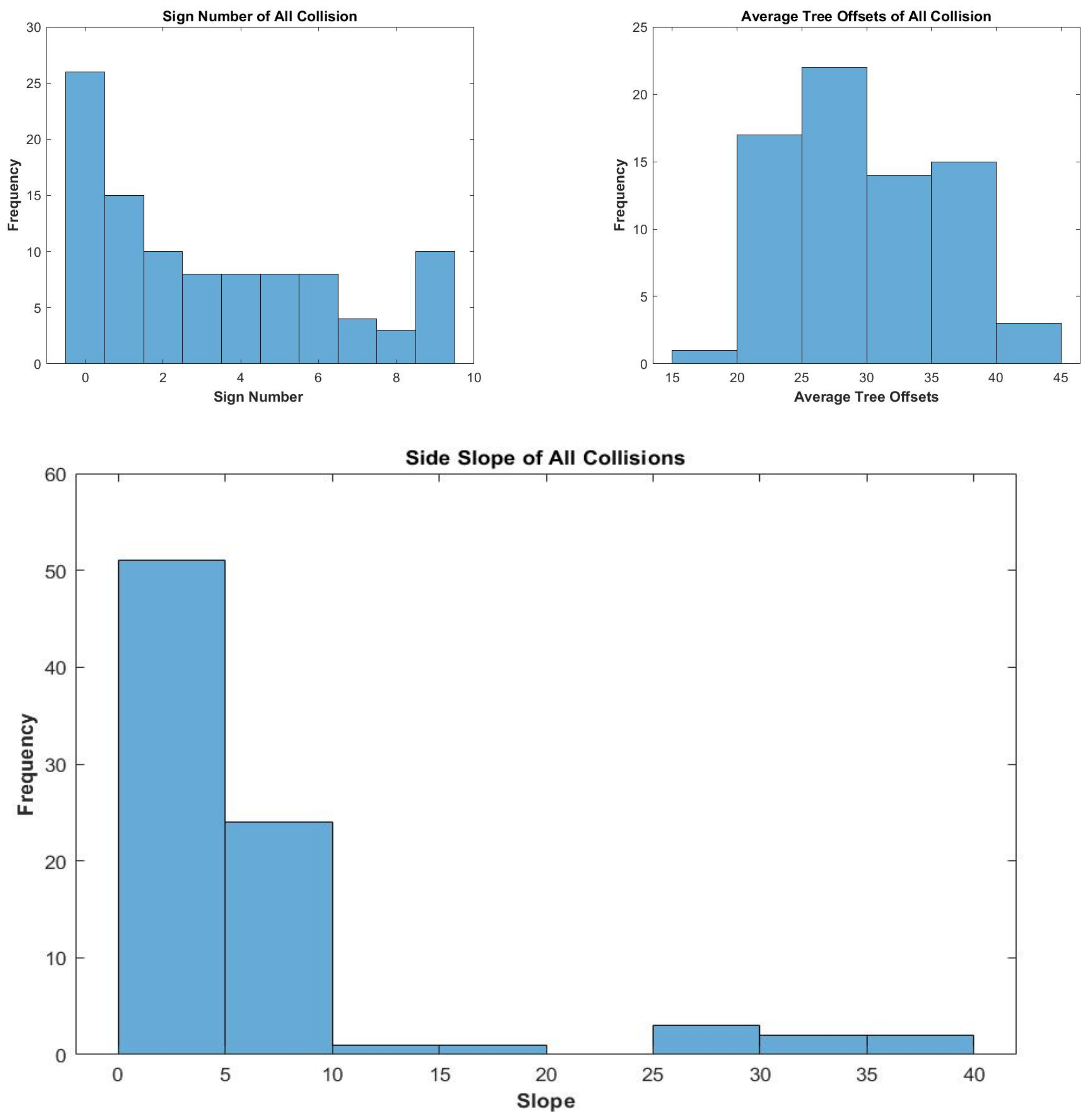
5.1. Variability in Extracted Features

Features extracted from LiDAR included attributes of poles, trees, side slopes, and traffic signs. This information was extracted in the vicinity of every fixed-object ROR collision that occurred on the crash-prone segments analyzed. Figure 7 shows the histograms of all the features that were extracted for each collision on the 80 km of highway analyzed. The plots demonstrate that roadside attributes within the vicinity of each collision event vary significantly across the different events. This indicates the importance of collecting data at a disaggregate collision level when performing safety diagnostics. Nevertheless, collecting this information using conventional surveying techniques on such a localized scale is often impractical. For instance, measuring side slopes, horizontal curve radii, or the offset of each utility pole at every collision location would be extremely challenging using conventional tools. As a result, some variables gathered in police reports are collected using visual inspection as opposed to actual measurements.

This paper demonstrates that combining high-resolution data capture using LiDAR with efficient data extraction algorithms allows for the large-scale extraction at a higher level of accuracy and in a more efficient manner. This helps safety analysts (i) work with more accurate information, (ii) constantly update their database with missing roadside information, and (iii) explore relationships between collisions and variables that had not been considered in the past due to data limitations.

5.2. Safety Assessment

To demonstrate the potential applications of the LiDAR extractions in roadside safety assessments, a secondary aim of this paper was to use the extracted information to explore links between the extracted attributes and the severity of ROR collisions.

Table 3. Final Regression Model.

	Estimate	S.E. a	Wald	df b	p-Value	OR c
Minimum Roadside Object Offset	−0.043	0.021	4.123	1	0.042 *	0.958
Side Slope Flatness	−0.086	0.047	3.326	1	0.068 *	0.918

^a S.E: Standard Error, ^b df: Degrees of Freedom, ^c OR: Odds Ratio, * Statistically significant at 90% confidence level.

shows the results of the logistic regression that was performed for that purpose. Before discussing the specific relationships, it is worth noting that goodness-of-fit statistics show that the model was a good fit for the data. Although the model was not intended for prediction, fit statistics also show that the model has very good predictive ability at 74% accuracy. The omnibus test shows a significant p-value of 0.000, which indicates that the independent variables are good predictors of the response.

For the specific relationships, the model shows that the offset of the nearest roadside object to the collision and the flatness of side slopes were the variables with the most statistically significant impacts on collision severity. It is worth noting here that the model was fit using a backward elimination strategy, where variables with insignificant effects were eliminated in a stepwise manner. Therefore, variables such as the number of poles, the existence of a tree canopy, and the spacing of pole-like objects were not found to have statistically significant impacts on the severity of fixed-object collisions. Since the model was testing the impacts on the severity of fixed-object ROR collisions as opposed to frequency, this finding is reasonable. In other words, although the increase in the number of roadside objects might impact the frequency of fixed-object ROR collisions, this is not expected to impact severity.

The existence of curve and curve radii (not in the final model) were also found to be insignificant. It is worth noting here that only 5 of the 10 curves found on the analyzed segment were sharper than 900 m, which is the radius considered to be critical in the Alberta Roadside Design Guide (i.e., accounting for the existence of a curve in roadside design only occurs if the radii exceed 900 m) [51]. Hence, there was limited variability in the sharpness of the curves in this study.

In the case of side slopes, the model shows that using flatter side slopes results in less severe ROR collisions. This is highly intuitive since steeper slopes often minimize the chances of recovery for errant vehicles. The results show that, at fixed unit height, increasing the width of a side slope by a single unit (i.e., moving from a 1:3 slope to a 1:4 slope) could reduce the chances of a fixed-object collision being severe by 8.2%. It is worth noting here that the Alberta Highway Design Guide warns that slopes between 1:4 and 1:3 may be traversable but not recoverable while recommending against using side slopes that are steeper than 1:4 [51]. Based on the assessment conducted in this study, only around 10% of the collisions had a side slope steeper than 1:3 in their vicinity.

Another significant variable was the minimum offset to the collision location. This variable was computed to overcome correlations between three different variables, namely, the average offset of the tree canopy, the average offset of poles, and the average offset of traffic signs within the vicinity of each collision. Hence, it represents the minimum average offset of all three types of roadside objects. The fact that this variable was found to be statistically significant shows that offsets seem to impact the severity of fixed-object ROR collisions regardless of the type of object. The model shows that a reduction in the offset (i.e., the closer the object is to the road) increases the likelihood of the collision being severe. The odds ratio shows that the severity increases by 4.2% for every meter reduction in the offset of the roadside object. This finding is consistent with existing research on roadside safety, which found that the utility pole offset had significant impacts on severity [9,33,38]. In addition, this paper shows that other roadside objects have an impact similar to utility poles when placed closer to the roadway.

Although the developed models only explored factors impacting the severity of fixed-object ROR collisions, work in this paper could be extended in many different areas. The fact that the paper demonstrates the ease with which roadside object inventory could be extracted from LiDAR means that further analysis of safety and design attributes could be conducted. For instance, future work could consider extending the developed models to include other features of the roadside environment or conducting a similar assessment on urban roads. Future work could also assess factors impacting the frequency of ROR collisions.

6. Summary and Conclusions

This paper utilizes LiDAR scans of highways for inventorying roadside information, including pole-like objects, signposts, tree canopies, side slopes, and horizontal curve radii for roadside safety assessments. The study then analyzes links between the extracted roadside features and the severity of fixed-object ROR collisions. The extraction is performed along 80 km of collision-prone highways in Alberta, where a total of 100 fixed-object collisions occurred. Each collision record is matched with roadside features in its vicinity, and logistic regression analysis is used to identify whether there is an association between roadside features and the severity of the collisions. The paper demonstrates how LiDAR data could be utilized for large-scale assessment of the impacts of roadside features on safety. This helps overcome data limitations and helps enrich safety assessments with recent information that reflects existing conditions on a roadway. The paper shows that the severity of collisions was mainly affected by the steepness of side slopes and the offset of roadside objects. In contrast, factors such as pole density and the existence of tree canopy did not impact collision severity.

Although the models did consider the impacts of multiple roadside features and their properties, collision-specific attributes were not considered, such as the driver’s use of restraint and the speed of the vehicle at the time of the collision. The study also did not consider the weather conditions at the time of the collision, which could impact the severity of ROR collisions. Unfortunately, most of this information was not available in collision reports and, hence, could not be included in the analysis, however, it is worth considering in future work. Future studies could also consider extending work in this paper to examine the feasibility of conducting a real-time collision risk assessment whereby geometric information surveyed using the LiDAR scan is immediately fed into a collision prediction model to assess collision risk.

That being said, the paper demonstrates the feasibility of utilizing LiDAR technology to perform comprehensive assessments of roadside safety for use in designing forgiving highways.

References

1. Alberta Transportation. Alberta Traffic Collision Statistics 2016; Publication Alberta Vehicle Geographical Statistics, Alberta Transportation, Office of Traffic Safety: Edmonton, AB, Canada, 2016. [Google Scholar]
2. Liu, C.; Ye, T.J. Run-Off-Road Crashes: An on-Scene Perspective; NHTSA: Washington, DC, USA, 2011; p. 36. [Google Scholar]
3. National Highway Traffic Safety Administration. Fatality Analysis Reporting System. Available online: https://cdan.nhtsa.gov/SASStoredProcess/guest (accessed on 27 July 2018).
4. AASHTO. A Policy on Geometric Design of Highways and Streets, 2011; American Association of State Highway Transportation Officials: Washington, DC, USA, 2011. [Google Scholar]
5. Bullough, J.D.; Donnell, E.T.; Rea, M.S. To illuminate or not to illuminate: Roadway lighting as it affects traffic safety at intersections. Accid. Anal. Prev. 2013, 53, 65–77. [Google Scholar] [CrossRef]
6. Bhagavathula, R.; Gibbons, R.B.; Edwards, C.J. Relationship between Roadway Illuminance Level and Nighttime Rural Intersection Safety. Transp. Res. Rec. J. Transp. Res. Board 2015, 2485, 8–15. [Google Scholar] [CrossRef]
7. El Esawey, M.; Sayed, T. Evaluating safety risk of locating above ground utility structures in the highway right-of-way. Accid. Anal. Prev. 2012, 49, 419–428. [Google Scholar] [CrossRef]
8. Hauer, E. An exemplum and its road safety morals. Accid. Anal. Prev. 2016, 94, 168–179. [Google Scholar] [CrossRef]
9. Lee, J.; Mannering, F. Impact of roadside features on the frequency and severity of run-off-roadway accidents: An empirical analysis. Accid. Anal. Prev. 2002, 34, 149–161. [Google Scholar] [CrossRef]
10. Yadav, M.; Lohani, B.; Singh, A.K.; Husain, A. Identification of pole-like structures from mobile lidar data of complex road environment. Int. J. Remote Sens. 2016, 37, 4748–4777. [Google Scholar] [CrossRef]
11. El-Halawany, S.I.; Lichti, D.D. Detecting road poles from mobile terrestrial laser scanning data. GIScience Remote Sens. 2013, 50, 704–722. [Google Scholar] [CrossRef]
12. Gargoum, S.A.; Koch, J.C.; El-Basyouny, K. A Voxel-Based Method for Automated Detection and Mapping of Light Poles on Rural Highways using LiDAR Data. Transp. Res. Rec. J. Transp. Res. Board 2018, 2672, 274–283. [Google Scholar] [CrossRef]
13. Wu, B.; Yu, B.; Yue, W.; Shu, S.; Tan, W.; Hu, C.; Huang, Y.; Wu, J.; Liu, H. A Voxel-Based Method for Automated Identification and Morphological Parameters Estimation of Individual Street Trees from Mobile Laser Scanning Data. Remote. Sens. 2013, 5, 584–611. [Google Scholar] [CrossRef] [Green Version]
14. Teo, T.-A.; Chiu, C.-M. Pole-Like Road Object Detection From Mobile Lidar System Using a Coarse-to-Fine Approach. IEEE J. Sel. Top. Appl. Earth Obs. Remote. Sens. 2015, 8, 4805–4818. [Google Scholar] [CrossRef]
15. Gargoum, S.; Karsten, L.; El-Basyouny, K. Network Level Clearance Assessment using LiDAR to Improve the Reliability and Efficiency of Issuing Over-Height Permits on Highways. Transp. Res. Rec. J. Transp. Res. Board 2018, 2672, 45–56. [Google Scholar] [CrossRef]
16. Gargoum, S.A.; Karsten, L. Virtual assessment of sight distance limitations using LiDAR technology: Automated obstruction detection and classification. Autom. Constr. 2021, 125, 103579. [Google Scholar] [CrossRef]
17. Gargoum, S.A.; El Basyouny, K. A literature synthesis of LiDAR applications in transportation: Feature extraction and geometric assessments of highways. GIScience Remote. Sens. 2019, 56, 864–893. [Google Scholar] [CrossRef]
18. Karsten, L.; Gargoum, S.; Saleh, M.; El-Basyouny, K. Automated Framework to Audit Traffic Signs Using Remote Sensing Data. J. Infrastruct. Syst. 2021, 27, 04021014. [Google Scholar] [CrossRef]
19. Zeybek, M. Extraction of Road Lane Markings from Mobile LiDAR Data. Transp. Res. Rec. J. Transp. Res. Board 2021. [Google Scholar] [CrossRef]
20. Hou, Q.; Ai, C. A network-level sidewalk inventory method using mobile LiDAR and deep learning. Transp. Res. Part C Emerg. Technol. 2020, 119, 102772. [Google Scholar] [CrossRef]
21. Che, E.; Olsen, M.J.; Jung, J. Efficient segment-based ground filtering and adaptive road detection from mobile light detection and ranging (LiDAR) data. Int. J. Remote. Sens. 2021, 42, 3633–3659. [Google Scholar] [CrossRef]
22. Wang, Z.; Yang, L.; Sheng, Y.; Shen, M. Pole-Like Objects Segmentation and Multiscale Classification-Based Fusion from Mobile Point Clouds in Road Scenes. Remote. Sens. 2021, 13, 4382. [Google Scholar] [CrossRef]
23. Gao, Z.; Doi, A.; Kato, T.; Takahashi, H.; Sakakibara, K.; Hosokawa, T.; Harada, M. Utility pole extraction processing from point cloud data from 3D measurement and its applications. In Proceedings of the 2020 11th International Conference on Awareness Science and Technology (iCAST); IEEE: Piscataway, NJ, USA, 2020; pp. 1–6. [Google Scholar]
24. Yang, B.; Dong, Z. A shape-based segmentation method for mobile laser scanning point clouds. ISPRS J. Photogramm. Remote. Sens. 2013, 81, 19–30. [Google Scholar] [CrossRef]
25. Lehtomäki, M.; Jaakkola, A.; Hyyppä, J.; Kukko, A.; Kaartinen, H. Detection of Vertical Pole-Like Objects in a Road Environment Using Vehicle-Based Laser Scanning Data. Remote. Sens. 2010, 2, 641–664. [Google Scholar] [CrossRef] [Green Version]
26. Pu, S.; Rutzinger, M.; Vosselman, G.; Elberink, S.O. Recognizing basic structures from mobile laser scanning data for road inventory studies. ISPRS J. Photogramm. Remote. Sens. 2011, 66, S28–S39. [Google Scholar] [CrossRef]
27. El-Halawany, S.I.; Lichti, D.D. Detection of Road Poles from Mobile Terrestrial Laser Scanner Point Cloud. In 2011 International Workshop on Multi-Platform/Multi-Sensor Remote Sensing and Mapping; IEEE: Piscataway, NJ, USA, 2011; pp. 1–6. [Google Scholar]
28. Yan, L.; Liu, H.; Tan, J.; Li, Z.; Xie, H.; Chen, C. Scan Line Based Road Marking Extraction from Mobile LiDAR Point Clouds. Sensors 2016, 16, 903. [Google Scholar] [CrossRef] [PubMed]
29. Lehtomäki, M.; Jaakkola, A.; Hyyppa, J.; Lampinen, J.; Kaartinen, H.; Kukko, A.; Puttonen, E.; Hyyppa, H. Object Classification and Recognition From Mobile Laser Scanning Point Clouds in a Road Environment. IEEE Trans. Geosci. Remote. Sens. 2016, 54, 1226–1239. [Google Scholar] [CrossRef] [Green Version]
30. Li, Y.; Wang, W.; Tang, S.; Li, D.; Wang, Y.; Yuan, Z.; Guo, R.; Li, X.; Xiu, W. Localization and Extraction of Road Poles in Urban Areas from Mobile Laser Scanning Data. Remote. Sens. 2019, 11, 401. [Google Scholar] [CrossRef] [Green Version]
31. Tu, J.; Yao, J.; Li, L.; Zhao, W.; Xiang, B. Extraction of Street Pole-Like Objects Based on Plane Filtering From Mobile LiDAR Data. IEEE Trans. Geosci. Remote. Sens. 2021, 59, 749–768. [Google Scholar] [CrossRef]
32. Li, J.; Cheng, X. Supervoxel-based extraction and classification of pole-like objects from MLS point cloud data. Opt. Laser Technol. 2022, 146, 107562. [Google Scholar] [CrossRef]
33. Jones, I.S.; Baum, A.S. An analysis of the urban utility pole accident problem. In Proceedings: American Association for Automotive Medicine Annual Conference, No. 22; Association for the Advancement of Automotive Medicine: Chicago, IL, USA, 1978; pp. 165–180. [Google Scholar]
34. Fox, J.C.; Good, M.C.; Joubert, P.N. Collisions with Utility Poles: Summary Report; Office of Road Safety, Commonwealth Department of Transport: Melbourne, Australia, 1979. [Google Scholar]
35. Mak, K.K.; Mason, R.L. Accident Analysis: Breakaway and Nonbreakaway Poles Including Sign and Light Standards along Highways; The Administration: Washington, DC, USA, 1980. [Google Scholar]
36. Zegeer, C.V.; Parker, P.M., Jr. Effect of traffic and roadway features on utility pole accidents. Transp. Res. Rec. 1984, 970, 65–76. [Google Scholar]
37. Good, M.; Fox, J.; Joubert, P. An in-depth study of accidents involving collisions with utility poles. Accid. Anal. Prev. 1987, 19, 397–413. [Google Scholar] [CrossRef]
38. Holdridge, J.M.; Shankar, V.N.; Ulfarsson, G.F. The crash severity impacts of fixed roadside objects. J. Saf. Res. 2005, 36, 139–147. [Google Scholar] [CrossRef]
39. Schneider, W.H.; Savolainen, P.T.; Zimmerman, K. Driver Injury Severity Resulting from Single-Vehicle Crashes along Horizontal Curves on Rural Two-Lane Highways. Transp. Res. Rec. J. Transp. Res. Board 2009, 2102, 85–92. [Google Scholar] [CrossRef]
40. Xie, Y.; Zhao, K.; Huynh, N. Analysis of driver injury severity in rural single-vehicle crashes. Accid. Anal. Prev. 2012, 47, 36–44. [Google Scholar] [CrossRef]
41. Park, J.; Abdel-Aty, M. Assessing the safety effects of multiple roadside treatments using parametric and nonparametric approaches. Accid. Anal. Prev. 2015, 83, 203–213. [Google Scholar] [CrossRef] [PubMed]
42. Roque, C.; Moura, F.; Cardoso, J.L. Detecting unforgiving roadside contributors through the severity analysis of ran-off-road crashes. Accid. Anal. Prev. 2015, 80, 262–273. [Google Scholar] [CrossRef] [PubMed]
43. RIEGL. RIEGL VMX-450 Data Sheet. RIEGL Laser Measurment Systems. Available online: http://www.riegl.com/uploads/tx_pxpriegldownloads (accessed on 1 April 2017).
44. Tawfeek, M.; El-Basyouny, K. Safety Prediction Modelling and Deployment of Safety Analyst Software; University of Alberta: Edmonton, AB, Canada, 2017. [Google Scholar]
45. Montella, A. A comparative analysis of hotspot identification methods. Accid. Anal. Prev. 2010, 42, 571–581. [Google Scholar] [CrossRef] [PubMed]
46. Chow, R.; Mah, J.; Duckworth, R.; Bielkiewicz, B.; Aoro, J.; Dunn, G.; Ekkelenkamp, D.; Latte, B.; Putz, H.; Shaflik, P. Alberta Highway Lighting Guide; Alberta Transportation: Edmonton, AB, Canada, 2003. [Google Scholar]
47. Gargoum, S.A.; El-Basyouny, K.; Froese, K.; Gadowski, A. A Fully Automated Approach to Extract and Assess Road Cross Sections From Mobile LiDAR Data. IEEE Trans. Intell. Transp. Syst. 2018, 19, 3507–3516. [Google Scholar] [CrossRef]
48. Gargoum, S.; El-Basyouny, K.; Sabbagh, J.; Froese, K. Automated Highway Sign Extraction Using Lidar Data. Transp. Res. Rec. J. Transp. Res. Board 2017, 2643, 1–8. [Google Scholar] [CrossRef] [Green Version]
49. Gargoum, S.; El-Basyouny, K.; Sabbagh, J. Automated extraction of horizontal curve attributes using LiDAR data. Transp. Res. Rec. J. Transp. Res. Board 2018, 2672, 98–106. [Google Scholar] [CrossRef]
50. Gargoum, S.A.; El-Basyouny, K.; Sabbagh, J. Assessing Stopping and Passing Sight Distance on Highways Using Mobile LiDAR Data. J. Comput. Civ. Eng. 2018, 32, 04018025. [Google Scholar] [CrossRef]
51. Alberta Transportation. Highway Geometric Design Guide; Alberta Transportation, Office of Traffic Safety: Edmonton, AB, Canada, 1999. [Google Scholar]
Figure 1. Map of highways assessed for fixed-object collisions.
Infrastructures 07 00007 g001
Figure 2. Isolated tree (Left) and group of trees/canopy (Right).
Infrastructures 07 00007 g002
Figure 3. Spread of points across neighboring voxels (plan view): (a) Pole-like Object; (b) Tree Canopy (Group of Trees).
Infrastructures 07 00007 g003
Figure 4. Non-ground objects: (a) full-segment; (b) tree canopy; (c) pole-like objects.
Infrastructures 07 00007 g004
Figure 5. Segmentation method proposed for pole-like object and tree canopy extraction.
Infrastructures 07 00007 g005
Figure 6. Roadside features within the buffer zone of collision: (a) collision with high density of roadside objects; (b) collision with low density of roadside objects.
Infrastructures 07 00007 g006aInfrastructures 07 00007 g006b
Figure 7. Variability in extracted features across different collision events.
Infrastructures 07 00007 g007aInfrastructures 07 00007 g007b