Abstract
The concept of Positive Energy Districts (PEDs) has emerged as a promising approach to achieving sustainable urban development. PEDs aim to balance the energy demand and supply within a district while reducing the carbon footprint and promoting renewable energy sources. Urban–Industrial Symbiosis (UIS) is another approach that involves the exchange of energy and resources between industrial processes and nearby urban areas to increase efficiency and reduce waste. Combining the concepts of PED and UIS can create self-sufficient, sustainable, and resilient districts. As the analysis and implementation of such systems are barely studied in North America, this research study was structured to fill the gap by evaluating the financial and environmental advantages of this combination. This study proposes a methodology to design a heat transmission system; then, it is applied to the case of a paper-making factory and a multifunctional heritage building in Montreal, Canada. The results show that the building’s new heating system can generate sufficient heat while emitting near-zero direct emissions. Overall, this paper argues that combining the concepts of PED and UIS can lead to a more sustainable and resilient urban area, and provides a roadmap for achieving this goal.
1. Introduction
Industrialization and urbanization have risen over recent years, increasing greenhouse gas (GHG) emissions [1]. Aligned with rising population and demand, the industrial sector has increased the extraction of raw materials and solid waste generation [2]. Industrial development is essential for provision of a high quality of life for society, and has a high economic significance [3]. As a result, finding solutions that decrease negative consequences while maintaining sustainability with economic growth is critical. In general, economic growth is unsustainable if it is assumed that the only way to increase GDP is by increasing production quantity. However, an alternative approach to GDP growth is to improve production efficiency, using less input material/energy to produce more product [4]. In the same way, the building sector plays a significant role in emitting GHG emissions. Buildings are responsible for almost 40% of global carbon dioxide emissions [5]. For many years, collections of methods have been introduced and tested to decrease the negative impact of this sector on climate change. Reducing fuel consumption and implementing electrification strategies are promising methods of reaching positive energy districts [6].
In 2015, the Paris agreement formalized action against climate change while highlighting the importance of finding sustainable solutions. However, a single solution is not possible for the myriad contextual differences that exist globally. Energy exchange between industries is one of many potential approaches to addressing the adverse impacts of human activity; in the literature, this is called industrial symbiosis (IS) [7]. For many years, IS has been a promising approach to responding to climate change [8]. The concept of IS is derived from industrial ecology, which proposes that an industrial system can be interconnected in ways mimicking natural systems, and realizing benefits from integration. From the systems view, it is more efficient for industrial facilities to work jointly in concerted actions. Industrial ecology focuses on the facility, inter-firm, and regional or global levels. Typically, IS studies integration potential at the inter-firm level [9].
IS contributes to the sustainable development of societies by addressing its three pillars (economic, environmental, and social), making IS a novel vehicle to achieve the United Nations Sustainable Development Goals (SDGs) [10]. Energy exchange in IS contributes to achieving SDG 7 by recovering excess heat of factories and supplying the energy demand of nearby facilities. Implementing IS decreases the waste and greenhouse gas emissions related to energy use. Generally, IS is limited to eco-industrial parks, because short distances are vital to IS; however, some studies have considered symbiosis between distant enterprises [11]. Although geographic proximity enables symbiosis between industries, if industrial facilities are close enough to the urban area, another term could emerge: urban–industrial symbiosis (UIS) [12,13].
Setting up an energy symbiosis network in a UIS provides the nearby building with ready-to-use excess heat. Such a network accelerates the process of reaching a PED in urban areas which are located near factories. However, this connection requires some prerequisite evaluation. First, technical feasibility examines the methods and technologies necessary to handle recovered energy. The second requirement explores economic, environmental, and social sustainability. Eventually, resiliency evaluates the long-term operation of the network under uncertainty [7]. This study focuses on the first and second steps.
Process heat in industries uses the largest share of the energy input, and almost half of this heat is above 500 °C [14]. High energy costs led to considerable improvements in energy efficiency in these industries over the past century. However, many industrial sites still release substantial amounts of lower-temperature energy into the environment. The excess heat released into the environment from the industrial sector should be further decreased, as far as possible, by energy efficiency measures in the individual industrial sites. It could also be utilized as a heat source in low-temperature district heating networks [15]. After analysis of relevant papers in UIS, below are two essential features of the recently published articles, methodology, and types of UIS:
Mathematical programming, pinch-based analysis, and evaluation are the most frequently used methods. Studies with mathematical programming mostly use mixed-integer linear programming (MILP) to find optimal solutions of decision variables regarding each problem’s characteristics. Among these studies, Kantor et al. [16] modeled and optimized material and energy symbiosis between factories, where urban areas could be considered as a sink for low-temperature heat. They also utilized the pinch analysis methodology to formulate heat cascade constraints while preserving the second law of thermodynamics. In 2022, Cunha et al. [17] evaluated the energy exchange of a waste-to-heat plant and a nearby district heating network (5 km distance). Their study claimed the proposed system achieved a 30% reduction in fuel consumption compared to the current condition. Simeoni et al. [18] developed a multi-objective optimization model to optimize the heat recovery decisions in the presence of factories and district heating networks. Ciotti et al. [19] developed a decision support system to facilitate decision makers in choosing the best heat recovery option. Nakama et al. [20] developed a dynamic optimization model to study the impact of thermal energy storage on system cost. Among others, some studies developed nonlinear models because of the hydraulic equations in optimization of the networks [21,22]. Finally, evaluation methods are broadly employed in the literature to measure the effectiveness of an existing or potential IS or UIS. For example, Kim et al. [23] measured the potential of using excess heat in an industrial park in Korea. They calculated the peak heat load of a regional urban area and assumed it as a sink site of excess heat. Ates and Ozcan [24] examined the excess heat in Turkey’s industries, and then studied the potential of power conversion technologies to decrease that heat loss.
Water, energy, and material are generally exchanged in IS and UIS. Energy can be decomposed into three forms: heating, cooling, and electricity. Material is usually defined as urban waste in a UIS network [17]; however, materials also include industrial co-products when considering IS networks. Yong et al. [25] integrated heating, cooling, and electricity exchange in UIS. The proposed method aimed to increase energy efficiency by 34% while utilizing the excess heat of the power plant in fulfilling residential demand. In 2021, Misrol et al. [26] designed a wastewater treatment network to reuse the recovered water from the urban area in the processes of factories.
Although many research projects have studied the role and impact of buildings in reaching a PED, this study aims to answer the question: how do industries take part in achieving a PED? Thus, this study is structured to study technical know-how and evaluate UIS’ capacity to realize a PED. This work is structured as follows: Section 2 explains the methodology and introduces the principles of all calculations. Section 3 introduces the case study and represents multiple heat recovery methods and their associated considerations. In addition, the current condition is compared to the proposed structures. Section 4 discusses the impact and limitations of this work. Finally, Section 5 concludes the study and provides potential directions for future research.
2. Materials and Methods
The proposed methodology evaluates the impact of recovering excess heat from industries and exchanging it with nearby buildings, which requires a heat transmission network and the installation of new units. The result is compared to the current state throughout the calculation of network variables. In this regard, Figure 1 shows the steps of the proposed methodology. The overall procedure consists of four steps:
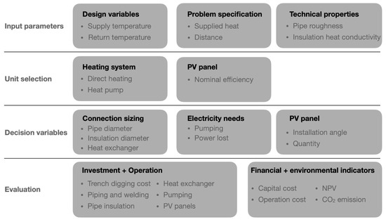
Figure 1.
Overview of the methodology.
In the first step, the required input data are gathered. Then, new energy systems are designed to reuse heat from industries; the goal is to reach a positive energy building that does not emit onsite emissions (Scope 1) and has lower Scope 2 emissions compared to the current state. Scope 1 refers to direct onsite emissions. For example, emissions associated with fuel combustion in a boiler are Scope 1 emissions. Scope 2 accounts for emissions from upstream activities. For instance, emissions that originate from a power plant are considered as Scope 2 emissions [27]. Next, the system is sized, and decision variables are estimated or optimized. Finally, the financial and environmental aspects are evaluated in the last phase. Later, five sub-sections explain the calculation of five essential parts: heat exchanger, connection pipes, photovoltaic (PV) panels, financial analysis, and environmental analysis.
2.1. Heat Exchanger Variables
Designing a heat exchanger is accompanied by defining many variables, which are shown in Figure 2. In most cases, the objective is to transfer the maximum amount of heat while preserving the required temperature difference on both sides of the heat exchanger.
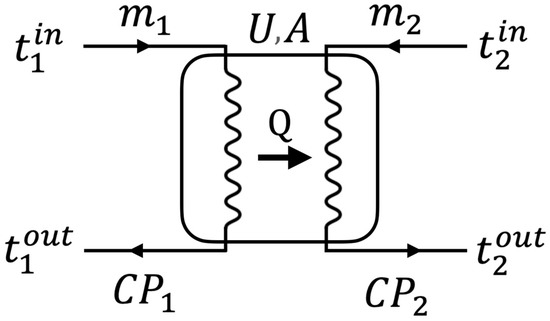
Figure 2.
Schematic view of a heat exchanger.
As shown in Figure 2, a simple heat exchanger consists of three major sections. The hot stream (index 1 in Figure 2) is the first component, which must cool down from to . In addition, and are the hot stream’s mass flow rate and specific heat capacity, respectively. The second part is the cold stream (index 2 in Figure 2), which must be heated from to . Finally, the heat exchanger unit is the last component, which is accompanied by two critical parameters, heat transfer coefficient () and surface area ().
As mentioned previously, a heat exchanger which transfers the maximum amount of heat () is the main objective of the design process. As a result, the following mathematical model, nonlinear programming (NLP), is structured, which finds a feasible solution () while satisfying the linear and non-linear constraints.
Equation (1) is the objective function and maximizes the amount of transferable heat in the heat exchanger. Equations (2) and (3) deal with the law of conservation of energy. Ultimately, Equation (4) limits the decision variables () into a reasonable interval, and is the minimum approach temperature in the heat exchanger.
2.2. Connection Variables
Transferring the excess energy from one site (e.g., a factory) to another (e.g., a building) requires installing pipes between them. The calculation of pipe diameter, pressure drop, and insulation thickness are further explained in this section. Table 1 introduces the parameters and variables utilized in the rest of this paper.

Table 1.
Input parameters and design variables of the model.
The required flow rate is calculated in the following equation:
Genic et al. [28] suggested the following equation for calculating the near-optimal pipe diameters (mm).
Equations (7)–(15) are used to calculate the pressure drop over the transmission line. The Kinematic viscosity and cross-sectional pipe area are calculated in Equations (3) and (4), which will be used later to calculate the Reynolds number.
Reynolds number is calculated in the following equation:
A numerical approximation method called Serghides’s solution [29] is used to estimate the friction factor. Equations (10)–(13) calculate this parameter.
The pressure drop is determined using the Darcy-Weisbach equation, considering the friction in the pipe, velocity of the fluid, and the length of the pipe:
Finally, the required pump power is calculated based on the pressure drop, flowrate, and pump efficiency:
Equations (16) and (17) calculate the transmission line’s heat loss and the insulation volume required to preserve the heat.
Equation (16) calculates heat losses over distance based on the conductivity of the insulator and the temperature difference between the pipes and the soil. Finally, Equation (17) calculates the volume of insulation needed to be installed. Insulation thickness is selected based on the work of Bahadori and Vuthaluru [30], which proposes a simple estimation model.
2.3. PV Panel
As a source of electricity generation, PV panels are among the most reliable and feasible solutions [31]. However, the installation location and available space strongly affect the output energy of this option. In this study, INSEL [32], an open-access simulation software, is applied to calculate the electricity generation of each PV panel. Weather data are an important input, providing various weather information specifically for each location; solar radiation is used, among the provided data. In the real world, solar radiation and temperature change quickly impact the power of PV panels. In this case, the maximum power point of a photovoltaic generator, MPP block, determines the maximum product of the naturally unimodal function . Figure 3 demonstrates other impactful parameters in energy generation. Tilt angle () and length () are calculated based on the installation latitude. Equation (18) calculates the distance () while is the solar radiation angle, or sun elevation, at noon of the shortest day of the year. (Figure 3).
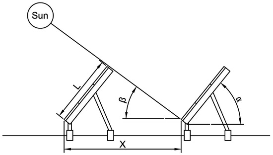
Figure 3.
Schematic view of PV panel installation properties.
2.4. Financial Analysis
The financial analysis is based on cash flow analysis. Two main types of cost in cash flow analysis are capital expenditure (CapEx) and operating expenditure (OpEx). The principal difference between these two is the time of payment. Typically, the former is paid once at the beginning of the project; the latter is repeated for each operating period. For example, equipment purchase costs are classified as CapEx, while the electricity consumption of the equipment is classified as OpEx.
As described previously, PV panels are the only component in this problem that generates onsite electricity (Table 2). Matching the electricity generation with onsite electricity demand is out of the scope of this work; therefore, it is assumed that the annual generated electricity is firstly consumed in the building, and the rest is sold to the electricity grid as revenue. Surplus PV power is assumed to be dispatched at the same rate as the supply rate from Hydro Quebec. This study calculates operation costs based on 0.097 for electricity [33] and 0.41 for natural gas consumption (including base, distribution, and service costs) [34].
Table 2.
Components of cash flow analysis.
Two metrics are evaluated through the financial analysis section. The first one is Net Present Value (NPV), which gives the current value of a future stream of payments. NPV is calculated by summing up the annual cash flow for the system’s lifetime and discounting with the interest rate. The second metric is Discounted Payback Period (DPP), which gives the years to recover the upfront investment cost, accounting for decreasing currency value. Table 3 describes the nomenclature of financial analysis.
Table 3.
Sets, parameters, and variables of financial analysis.
Equation (19) calculates of positive and negative cash flows by discounting all inflows and outflows to the present (the base year).
DPP finds the minimum years required to gain a positive NPV. It shows how fast the investment will be recovered throughout the years. The following shows the steps to find the DPP:
- Initial investment cost: this is the money required to invest.
- Cash inflows: this is the amount of cash the investment is expected to generate over its useful life.
- Discounted cash inflows: this involves discounting each cash inflow from the investment by the appropriate discount rate.
- Calculate the cumulative discounted cash inflows: this involves adding the “number 3” until they equal the initial investment cost.
- Determine the discounted payback period: this is the time it takes for the cumulative discounted cash inflows to equal the initial investment cost.
2.5. Environmental Analysis
This study evaluates Scope 1 and Scope 2 GHG emissions. The total GHG emissions are the sum of the two. This is because Scope 1 emissions are direct emissions from sources owned or controlled by the reporting organization. In contrast, Scope 2 emissions are indirect emissions from the generation of purchased electricity, heat, or steam consumed by the customer. This study converts all emissions to the same scale, equivalents. The following equation calculates this parameter:
In Equation (20), is the set of fuels (e.g., natural gas), and is the global warming potential associated with fuel consumption . In addition, is the set of electricity sources (e.g., hydro or solar), and is the electricity emission rate related to source . Note that total emission is summed over , which is determined based on the research goal.
3. Case Study
The proposed method is applied to a multifunctional building in Montreal. This building is pursuing zero emission by electrifying the heating system. Meanwhile, a paper-making factory (Kruger, Place Turcot Mill) is located near that building (), which is an appropriate case for energy exchange. The building’s heating load is provided by the owner based on a historical analysis, which had been derived from a simulation model. Figure 4 shows the heating load throughout the year. In this section, net present value is calculated for the period of 20 years, and discount rate is derived based on current and historical data in the Bank of Canada [35].
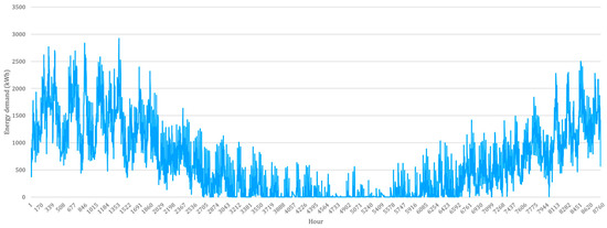
Figure 4.
Hourly heating load.
3.1. Unit Selection and Sizing
Selecting the correct heating system for a building is crucial for achieving comfortable indoor temperatures while minimizing energy consumption and cost. While the local climate, unit availability, and serviceability are vital factors, the owner’s strategy has more priority. Since the building aims to become carbon neutral, several units are considered appropriate candidates. Direct heating from the nearby factory, heat pump, and electric boiler are among the options which do not include Scope 1 emissions. In this study, different scenarios are generated based on the combination of units; then, the result is compared to assist key stakeholders in reaching a final decision. Note that the heat distribution network is excluded from the analysis. As such, the evaluation phase does not consider the modification of the piping network inside the building.
3.2. Heating System Sizing
3.2.1. Scenario 0, Present Condition
Two steam boilers and a backup boiler cover the building’s heating demand. Natural gas is the fuel source; as a result, direct emissions are implied in this scenario. Based on the Canada energy conversion tables [36], and by assuming 88% efficiency of the steam boilers, natural gas is consumed in this scenario. Figure 5 represents the current condition, where the warm wastewater in the paper making factory has not been integrated.
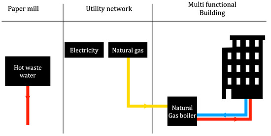
Figure 5.
Configuration of the actual case.
3.2.2. Scenario 1, PV Installation
Figure 6 indicates the scope and detail of the network in the first scenario. It shows how PV panel installation will impact the energy consumption in the building. This scenario provides the principal calculation of PV panels and their capacity to generate electricity. Subsequently, the result phase shows the financial analysis of the PV panel installation.
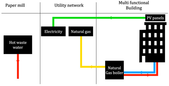
Figure 6.
Configuration of Scenario 1.
Based on the Canadian PV panel market availability, model CS5P-240 manufactured by Canadian Solar Inc. is selected for installation [37]. The dimensions of the selected PV panel are 1.6 m × 1.0 m with nominal power of 240 W and nominal efficiency of 14.12%. Rowlands et al. [38] investigated the optimum PV tilt in Ottawa and Toronto. They found 38° as the optimal tilt in Ottawa. This study uses this number, as Montreal and Ottawa have almost the same latitude. The distance (X, in Figure 3) is calculated using Equation (18) to be 3.75 m; this prevents panels from shading each other in the winter.
The roof and installation layout, with 100% coverage, is shown in Figure 7. In this figure, each rectangle represents three bundled solar panels (width: 3 m, height: 1.6 m). In fact, the total roof area is not available for installation purposes. However, based on the site visit, almost 90% of the roof area is suitable. As a result, 2485 panels may be installed.
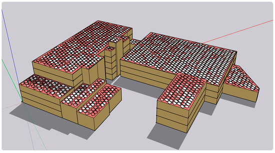
Figure 7.
Panels installation layout based on 100% coverage.
After implementing the model in INSEL, the hourly energy of PV panels is calculated and presented in Figure 8. As an output, all panels generate 931 MWh annually.
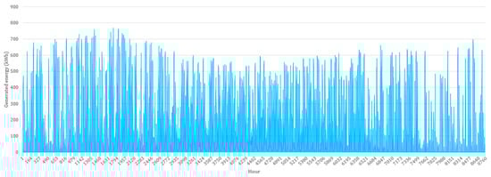
Figure 8.
Electricity generation of PV panels over one year.
3.2.3. Scenario 2, Direct Heating
In this scenario, the heat exchanger in the paper-making factory transfers the excess heat to the medium in the pipeline, which will be directly supplied to the building. Figure 9 shows the new scope and configuration. IPOPT [39], an open-source solver, was selected to optimize the NLP model. Table 4 summarizes parameters and decision variables derived from the optimization model and evaluation. In this scenario, 700 kW of power is delivered to the building through four-inch pipes (supply and return).
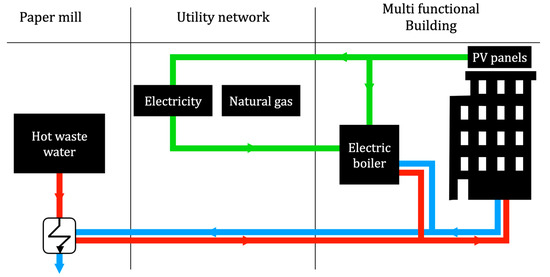
Figure 9.
Configuration in Scenario 2.
Table 4.
Design parameters of Scenario 2.
In this scenario, direct heating serves as the primary source of the heating system. It is sufficient to provide enough heat for 60% of the heating demand. The remaining 40% is provided by integrating the electric boiler into the system. Figure 10 shows the status of two designed units. Direct heating requires energy for pumping the medium along the network, , and the electric boiler consumes . After deduction, the electricity generated by PV panels, , is imported from the utility grid.
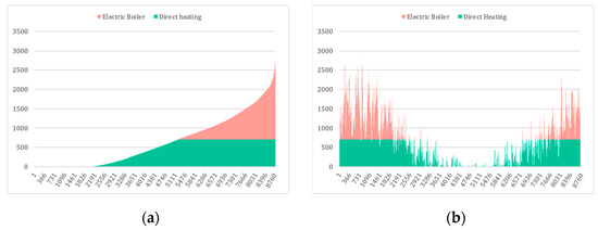
Figure 10.
Heating demand supplied from industrial excess heat (60%) and electric boiler (40%): (a) sorted based on the energy; (b) sorted hourly (1 January–31 December).
3.2.4. Scenario 3, Heat Pump
Figure 11 shows the configuration for Scenario 3, which leverages the use of a heat pump. The heat exchanger in the paper-making factory transfers the excess heat to the water in the pipeline, which will be utilized in the heat pump. Table 5 summarizes parameters and decision variables derived from the optimization model and evaluation. In this scenario, the input temperature to the heat pump is far lower than in the previous scenario; as a result, more power is recovered. The connection network delivers to the heat pump evaporator.
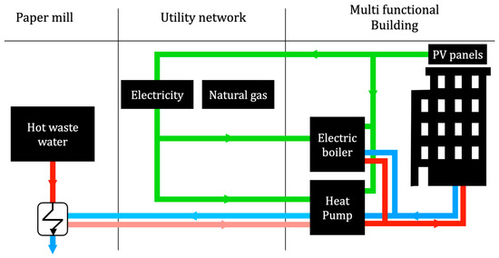
Figure 11.
Configuration in Scenario 3.
Table 5.
Design parameters of Scenario 3.
In this scenario, the heat pump plays a central role in heating the building. A heat pump with 1800 kW capacity provides 94% of the energy demand in this case. In the same way as the first scenario, the rest, 6%, is provided by integrating the electric boiler into the system. Figure 12 shows the coverage of each proposed unit in a year. The advantage of this scenario is the presence of a heat pump with a high coefficient of performance (COP). Based on this observation, Johnson Controls company [44] manufactures industrial heat pumps that match the excess heat recovery network. Among various models, “NS Heat Pump 193 HP” is selected, which offers COP 3.9 in the designed condition. Scenario 3 includes more components than Scenario 2, but has lower electricity consumption. Here, the heat pump consumes , the pumps consume , and the electric boiler consumes . After deducting the generated electricity, of energy is required from the utility grid.
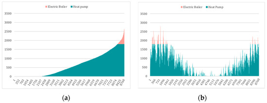
Figure 12.
Heating demand supplied from heat pump (94%) and electric boiler (6%): (a) sorted based on the energy; (b) sorted based on date (1 January–31 December).
3.2.5. Scenario 4, Heat Pump without PV Panels
Scenario 4 resembles Scenario 3; however, the PV panels are excluded from the retrofit plan. This scenario examines the advantage of utilizing excess heat combined with the heat pump unit. In this system, Scope 1 emissions are zero regarding the electrification of the heating system. Moreover, due to the presence of Hydro Quebec electricity, Scope 2 emissions are far lower than the electricity generated by power plants. In contrast, the building loses the ability to generate electricity and does not dispatch the surplus electricity to the grid. In other words, the building cannot send energy into the district.
3.3. Evaluation
Each scenario was evaluated for financial performance based on the defined economic metrics. The first scenario does not require a circulation pump, and therefore does not consume electricity as part of the heating system. Based on this fact, Table 5 summarizes all scenarios’ CapEx, OpEx, and Revenue. The most critical parameter of the operation phase is the utility rate, introduced in the methodology section, which is then cross-checked with the actual bills. In addition, the “Heat transmission line” is made of these items: pipe cost, insulation cost, and installation cost. Table 6 demonstrates the PV panel’s considerable capital cost, which is necessary to achieve a zero emission building.
Table 6.
Financial analysis of all scenarios.
In order to calculate the financial metrics, NPV and DPP, the definition of the revenue is important. In this case, operation costs in Scenario 0 are considered the base of calculation, and economization by implementing other scenarios is considered the revenue, aside from the revenue of selling generated electricity. Table 7 concludes the result of the evaluation phase and reports all metrics introduced in the methodology section.
Table 7.
Financial and environmental metrics.
4. Discussion
The final evaluation showed that reaching nearly zero emission is possible, not only through the electrification of the heating system, but also by recovering excess heat from factories and transferring it to nearby buildings or districts. Scenario 1 represents that PV panel installation alone does not seem appealing for owners, with a payback period of more than 25 years. However, when the self-generation strategy is aligned with the zero-emission building strategy, Scenario 3 becomes more interesting. In this case, the building’s CO2 footprint for heating approaches zero. Moreover, surplus electricity from PV panels is injected into the grid, providing electricity to the district. Scenario 2 may be selected with a short-term planning horizon, as the heating system has a lower capital cost (32%) compared to Scenario 3. However, for long-term planning, it performs worse than Scenario 3, based on the high OpEx. Finally, Scenario 4 demonstrates better financial metrics compared to the others. Electrification of the heating system emits less than 5% of the current emissions because of the low-emission electricity source (hydro). The capital and operation costs are recovered in only 8 years, which motivates the building’s owner to invest in this scenario.
There are two limitations associated with this study. First, the wastewater temperature at the factory is uncertain. There is a possibility that Scenario 2 cannot be implemented because of low-temperature wastewater. For example, when the temperature drops to 40 °C, the potential for direct heating declines. In that case, Scenario 3 still works with a lower heat capacity, and electricity consumption decreases because of the lower COP. However, the heat pump specification and its capacity to utilize a low temperature medium impact decision-making. Physical realization of the systems, such as piping placement, is another general limitation. The shortest distance between supplier and demand should be used, though site-specific restrictions (public or private land) may cause the piping length to increase. The distance of 800 m considered in the case study includes foreseeable conditions, but further pursuit of the project may yield additional complications. Finally, examination of the heat distribution system in the building was excluded from this study, which needs further investigation on the supply temperature inside the building.
5. Conclusions
This study aimed to investigate the feasibility of exchanging industrial excess heat with nearby buildings for space heating. The study proposed a technical evaluation method to analyze the feasibility of such a network. The method was applied to a case study of a paper-making factory near a large building with a high heating demand in a cold climate. One motivation to examine this case study was the zero-emission strategy of the building.
Through a series of optimization problems, along with technical and economic analyses, this study demonstrated that exchanging industrial waste heat with a nearby building could result in significant energy savings for the building. The calculation showed that the excess heat could be used to provide up to 60% of the heating demand in the direct heating scenario, and up to 94% with the installation of a heat pump.
Economic analyses also indicated that implementing such a system (a heat pump without PV panels) would be financially feasible for the building, with payback periods of 8 years. Moreover, the possibility of a nearly zero-emission building was shown, which increased the investment payback period to 16 years. However, the study also highlighted some technical and operational challenges that must be addressed to implement such a system successfully. These include ensuring a match between the temperature and quality of the excess heat and the building’s heating demand, as well as establishing a reliable and efficient heat transfer system.
In conclusion, the study demonstrated that exchanging industrial waste heat with a nearby building can be a viable and cost-effective way to meet energy demands while reducing greenhouse gas emissions. Future research should address the technical and operational challenges associated with the energy storage concept for both electricity and heat, which ultimately impacts the system’s operation. In this study, different scenarios were defined and evaluated; however, in a complex network with multiple factories and buildings, the number of scenarios increases drastically, so formulating an optimization model to find a set of optimal solutions under different contextual settings would provide a more generalizable approach. The optimization model can include one or multiple objectives: economic, environmental, and social. The solutions may be analyzed with different methods, for example, the Pareto frontier, which provides decision-makers an overview of the optimum solutions.
Author Contributions
Conceptualization, E.S.R.; methodology, E.S.R.; validation, E.S.R.; writing—original draft preparation, E.S.R.; writing—review and editing, E.S.R., U.E., I.K. and R.P.M.; supervision, U.E. and I.K.; project administration, U.E.; funding acquisition, U.E. All authors have read and agreed to the published version of the manuscript.
Funding
This research was funded by Canada Excellence Research Chair in Smart, Sustainable and Resilient Communities and Cities and funded by Tri-Agency Institutional Program Secretariat.
Data Availability Statement
Data will be available upon request.
Acknowledgments
The authors would like to express their appreciation to the Canada Excellence Research Chairs Program. In addition, the authors would like to extend their sincere gratitude to Ahmad Tavajohi Birjandi, whose feedback and suggestions were immensely helpful in refining the content.
Conflicts of Interest
The authors declare no conflict of interest. The funders had no role in the design of the study; in the collection, analyses, or interpretation of data; in the writing of the manuscript; or in the decision to publish the results.
References
- Dong, F.; Wang, Y.; Su, B.; Hua, Y.; Zhang, Y. The Process of Peak CO2 Emissions in Developed Economies: A Perspective of Industrialization and Urbanization. Resour. Conserv. Recycl. 2019, 141, 61–75. [Google Scholar] [CrossRef]
- Guan, Y.; Huang, G.; Liu, L.; Zhai, M.; Zheng, B. Dynamic Analysis of Industrial Solid Waste Metabolism at Aggregated and Disaggregated Levels. J. Clean. Prod. 2019, 221, 817–827. [Google Scholar] [CrossRef]
- Haraguchi, N.; Martorano, B.; Sanfilippo, M. What Factors Drive Successful Industrialization? Evidence and Implications for Developing Countries. Struct. Chang. Econ. Dyn. 2019, 49, 266–276. [Google Scholar] [CrossRef]
- Feldstein, M. Underestimating the Real Growth of GDP, Personal Income, and Productivity. J. Econ. Perspect. 2017, 31, 145–164. [Google Scholar] [CrossRef]
- Directorate-General for Energy (European Commission). Clean Energy for All Europeans; Publications Office of the European Union: Luxembourg, 2019; ISBN 978-92-79-99835-5. [Google Scholar]
- Hedman, Å.; Rehman, H.U.; Gabaldón, A.; Bisello, A.; Albert-Seifried, V.; Zhang, X.; Guarino, F.; Grynning, S.; Eicker, U.; Neumann, H.-M.; et al. IEA EBC Annex83 Positive Energy Districts. Buildings 2021, 11, 130. [Google Scholar] [CrossRef]
- Afshari, H.; Tosarkani, B.M.; Jaber, M.Y.; Searcy, C. The Effect of Environmental and Social Value Objectives on Optimal Design in Industrial Energy Symbiosis: A Multi-Objective Approach. Resour. Conserv. Recycl. 2020, 158, 104825. [Google Scholar] [CrossRef]
- Fan, Y.; Qiao, Q.; Fang, L.; Yao, Y. Emergy Analysis on Industrial Symbiosis of an Industrial Park—A Case Study of Hefei Economic and Technological Development Area. J. Clean. Prod. 2017, 141, 791–798. [Google Scholar] [CrossRef]
- Chertow, M.R. Industrial Symbiosis: Literature and Taxonomy. Annu. Rev. Energy. Environ. 2000, 25, 313–337. [Google Scholar] [CrossRef]
- Envision2030: 17 Goals to Transform the World for Persons with Disabilities|United Nations Enable. Available online: https://www.un.org/development/desa/disabilities/%20envision2030.html (accessed on 5 March 2023).
- Yu, C.; de Jong, M.; Dijkema, G.P.J. Process Analysis of Eco-Industrial Park Development—The Case of Tianjin, China. J. Clean. Prod. 2014, 64, 464–477. [Google Scholar] [CrossRef]
- Chen, X.; Fujita, T.; Ohnishi, S.; Fujii, M.; Geng, Y. The Impact of Scale, Recycling Boundary, and Type of Waste on Symbiosis and Recycling. J. Ind. Ecol. 2012, 16, 129–141. [Google Scholar] [CrossRef]
- Berkel, R.V.; Fujita, T.; Hashimoto, S.; Fujii, M. Quantitative Assessment of Urban and Industrial Symbiosis in Kawasaki, Japan. Environ. Sci. Technol. 2009, 43, 1271–1281. [Google Scholar] [CrossRef]
- Rehfeldt, M.; Fleiter, T.; Toro, F. A Bottom-up Estimation of the Heating and Cooling Demand in European Industry. Energy Effic. 2018, 11, 1057–1082. [Google Scholar] [CrossRef]
- Xu, Z.Y.; Wang, R.Z.; Yang, C. Perspectives for Low-Temperature Waste Heat Recovery. Energy 2019, 176, 1037–1043. [Google Scholar] [CrossRef]
- Kantor, I.; Robineau, J.-L.; Bütün, H.; Maréchal, F. A Mixed-Integer Linear Programming Formulation for Optimizing Multi-Scale Material and Energy Integration. Front. Energy Res. 2020, 8, 49. [Google Scholar] [CrossRef]
- Cunha, J.M.; Faria, A.S.; Soares, T.; Mourão, Z.; Nereu, J. Decarbonization Potential of Integrating Industrial Excess Heat in a District Heating Network: The Portuguese Case. Clean. Energy Syst. 2022, 1, 100005. [Google Scholar] [CrossRef]
- Simeoni, P.; Ciotti, G.; Cottes, M.; Meneghetti, A. Integrating Industrial Waste Heat Recovery into Sustainable Smart Energy Systems. Energy 2019, 175, 941–951. [Google Scholar] [CrossRef]
- Ciotti, G.; Cottes, M.; Mazzolini, M.; Sappa, A.; Simeoni, P. A decision Support System for Industrial Waste Heat Recovery: The CE-HEAT Project. In Proceedings of the Summer School F. Turco—Industrial Systems Engineering, Brescia, Italy, 11–13 September 2019. [Google Scholar]
- Nakama, C.S.M.; Knudsen, B.R.; Tysland, A.C.; Jäschke, J. A Simple Dynamic Optimization-Based Approach for Sizing Thermal Energy Storage Using Process Data. Energy 2023, 268, 126671. [Google Scholar] [CrossRef]
- Pan, M.; Sikorski, J.; Akroyd, J.; Mosbach, S.; Lau, R.; Kraft, M. Design Technologies for Eco-Industrial Parks: From Unit Operations to Processes, Plants and Industrial Networks. Appl. Energy 2016, 175, 305–323. [Google Scholar] [CrossRef]
- Pang, K.Y.; Liew, P.Y.; Woon, K.S.; Ho, W.S.; Wan Alwi, S.R.; Klemeš, J.J. Multi-Period Multi-Objective Optimisation Model for Multi-Energy Urban-Industrial Symbiosis with Heat, Cooling, Power and Hydrogen Demands. Energy 2023, 262, 125201. [Google Scholar] [CrossRef]
- Kim, H.-W.; Dong, L.; Choi, A.E.S.; Fujii, M.; Fujita, T.; Park, H.-S. Co-Benefit Potential of Industrial and Urban Symbiosis Using Waste Heat from Industrial Park in Ulsan, Korea. Resour. Conserv. Recycl. 2018, 135, 225–234. [Google Scholar] [CrossRef]
- Ates, F.; Ozcan, H. Turkey’s Industrial Waste Heat Recovery Potential with Power and Hydrogen Conversion Technologies: A Techno-Economic Analysis. Int. J. Hydrogen Energy 2022, 47, 3224–3236. [Google Scholar] [CrossRef]
- Yong, W.N.; Liew, P.Y.; Woon, K.S.; Wan Alwi, S.R.; Klemeš, J.J. A Pinch-Based Multi-Energy Targeting Framework for Combined Chilling Heating Power Microgrid of Urban-Industrial Symbiosis. Renew. Sustain. Energy Rev. 2021, 150, 111482. [Google Scholar] [CrossRef]
- Misrol, M.A.; Wan Alwi, S.R.; Lim, J.S.; Manan, Z.A. An Optimal Resource Recovery of Biogas, Water Regeneration, and Reuse Network Integrating Domestic and Industrial Sources. J. Clean. Prod. 2021, 286, 125372. [Google Scholar] [CrossRef]
- US EPA. Scope 1 and Scope 2 Inventory Guidance. Available online: https://www.epa.gov/climateleadership/scope-1-and-scope-2-inventory-guidance (accessed on 8 March 2023).
- Genić, S.B.; Jaćimović, B.M.; Genić, V.B. Economic Optimization of Pipe Diameter for Complete Turbulence. Energy Build. 2012, 45, 335–338. [Google Scholar] [CrossRef]
- Serghides, T.K. Estimate Friction Factor Accurately. Chem. Eng. 1984, 91, 63–64. [Google Scholar]
- Bahadori, A.; Vuthaluru, H.B. A Simple Correlation for Estimation of Economic Thickness of Thermal Insulation for Process Piping and Equipment. Appl. Therm. Eng. 2010, 30, 254–259. [Google Scholar] [CrossRef]
- Panwar, N.L.; Kaushik, S.C.; Kothari, S. Role of Renewable Energy Sources in Environmental Protection: A Review. Renew. Sustain. Energy Rev. 2011, 15, 1513–1524. [Google Scholar] [CrossRef]
- INSEL—Homepage—INSEL En. Available online: https://www.insel.eu/en/home_en.html (accessed on 5 March 2023).
- Rate D. Available online: https://www.hydroquebec.com/residential/customer-space/rates/rate-d.html (accessed on 9 March 2023).
- Price and Evolution|Énergir. Available online: https://www.energir.com/en/major-industries/natural-gas-price/price-and-evolution/ (accessed on 3 April 2023).
- Policy Interest Rate. Available online: https://www.bankofcanada.ca/core-functions/monetary-policy/key-interest-rate/ (accessed on 3 April 2023).
- Energy Conversion Tables—Canada.Ca. Available online: https://apps.cer-rec.gc.ca/Conversion/conversion-tables.aspx#s1ss2 (accessed on 8 March 2023).
- CSI Solar–Global. Available online: https://www.csisolar.com/ (accessed on 19 April 2023).
- Rowlands, I.H.; Kemery, B.P.; Beausoleil-Morrison, I. Optimal Solar-PV Tilt Angle and Azimuth: An Ontario (Canada) Case-Study. Energy Policy 2011, 39, 1397–1409. [Google Scholar] [CrossRef]
- Ipopt: Documentation. Available online: https://coin-or.github.io/Ipopt/ (accessed on 8 March 2023).
- Bengtsson, C.; Nordman, R.; Berntsson, T. Utilization of Excess Heat in the Pulp and Paper Industry—A Case Study of Technical and Economic Opportunities. Appl. Therm. Eng. 2002, 22, 1069–1081. [Google Scholar] [CrossRef]
- Manz, P.; Kermeli, K.; Persson, U.; Neuwirth, M.; Fleiter, T.; Crijns-Graus, W. Decarbonizing District Heating in EU-27 + UK: How Much Excess Heat Is Available from Industrial Sites? Sustainability 2021, 13, 1439. [Google Scholar] [CrossRef]
- Ovchinnikov, P.; Borodiņecs, A.; Strelets, K. Utilization Potential of Low Temperature Hydronic Space Heating Systems: A Comparative Review. Build. Environ. 2017, 112, 88–98. [Google Scholar] [CrossRef]
- Bergman, T.L. (Ed.) Introduction to Heat Transfer, 6th ed.; Wiley: Hoboken, NJ, USA, 2011; ISBN 978-0-470-50196-2. [Google Scholar]
- Johnson Controls. Available online: https://www.johnsoncontrols.com:443/ (accessed on 9 March 2023).
- Horizontal Close Coupled Centrifugal Water Pump and Standardized F40/125A 2.2 kW. Available online: https://www.tomeiwatersolutions.com/en/home/water-pumps/pedrollo/centrifugal/standard-centrifugal-according-to-en733/horizontal-close-coupled-centrifugal-water-pump-and-standardized-f40-125a-2-2kw.2.5.231.gp.38427.uw (accessed on 3 April 2023).
- Cost of Solar Power In Canada. 2021. Available online: https://www.energyhub.org/cost-solar-power-canada/ (accessed on 3 April 2023).
- Complete Boiler Room Solutions|Cleaver-Brooks. Available online: https://cleaverbrooks.com/ (accessed on 3 April 2023).
- More Positions in Canada. Available online: https://www.alfalaval.ca/ (accessed on 3 April 2023).
- Jossen, A.; Garche, J.; Sauer, D.U. Operation Conditions of Batteries in PV Applications. Solar Energy 2004, 76, 759–769. [Google Scholar] [CrossRef]
- Environment and Climate Change Canada (ECCC). Emission Factors and Reference Values. Available online: https://www.canada.ca/en/environment-climate-change/services/climate-change/pricing-pollution-how-it-will-work/output-based-pricing-system/federal-greenhouse-gas-offset-system/emission-factors-reference-values.html (accessed on 9 March 2023).
- GHG Emissions and Electricity|Hydro-Québec. Available online: https://www.hydroquebec.com/sustainable-development/specialized-documentation/ghg-emissions.html (accessed on 9 March 2023).
Disclaimer/Publisher’s Note: The statements, opinions and data contained in all publications are solely those of the individual author(s) and contributor(s) and not of MDPI and/or the editor(s). MDPI and/or the editor(s) disclaim responsibility for any injury to people or property resulting from any ideas, methods, instructions or products referred to in the content. |
© 2023 by the authors. Licensee MDPI, Basel, Switzerland. This article is an open access article distributed under the terms and conditions of the Creative Commons Attribution (CC BY) license (https://creativecommons.org/licenses/by/4.0/).