1. Introduction
Temporally and spatially correlated stimuli can be used for multifocal electroretinography (mfERG), in contrast to the conventional use of independent stimulus elements modulated with temporally white luminance sequences [
1,
2,
3]. These correlations must be discounted in order to properly assign credit for responses to the stimulus elements that caused those responses [
4,
5,
6,
7,
8,
9].
Eye movements can also be allowed, as opposed to requiring steady fixation [
3,
10]. Two problems emerge because of the presence of eye movements during recording. Each saccade evokes an artifactual signal that interferes with recording the desired retinal activity. These artifacts need to be discounted [
3,
11]. In addition, movement of the eyes across the stimulus moves the stimulus across the retina, so analyses can no longer be performed in stimulus coordinates. Instead, analyses must take place in retinotopic coordinates, and the stimulus modulations over time must be computed based on known stimulus and eye position records.
We show briefly that temporally natural stimuli can be used, and primarily address questions involving spatial issues. Can accurate mfERGs be obtained in the presence of eye movements? Can results be obtained in reasonable sampling times?
This work might lead to additional capabilities of mfERG, especially in testing younger and older patients more effectively. Eventually, it may be possible to evaluate geographic retinal function by letting patients watch natural movies. The general goals are to make mfERG more patient-friendly, more natural, more quantitative, and easier for the clinician to interpret.
3. Discussion
3.1. Temporal Statistics and Contrast
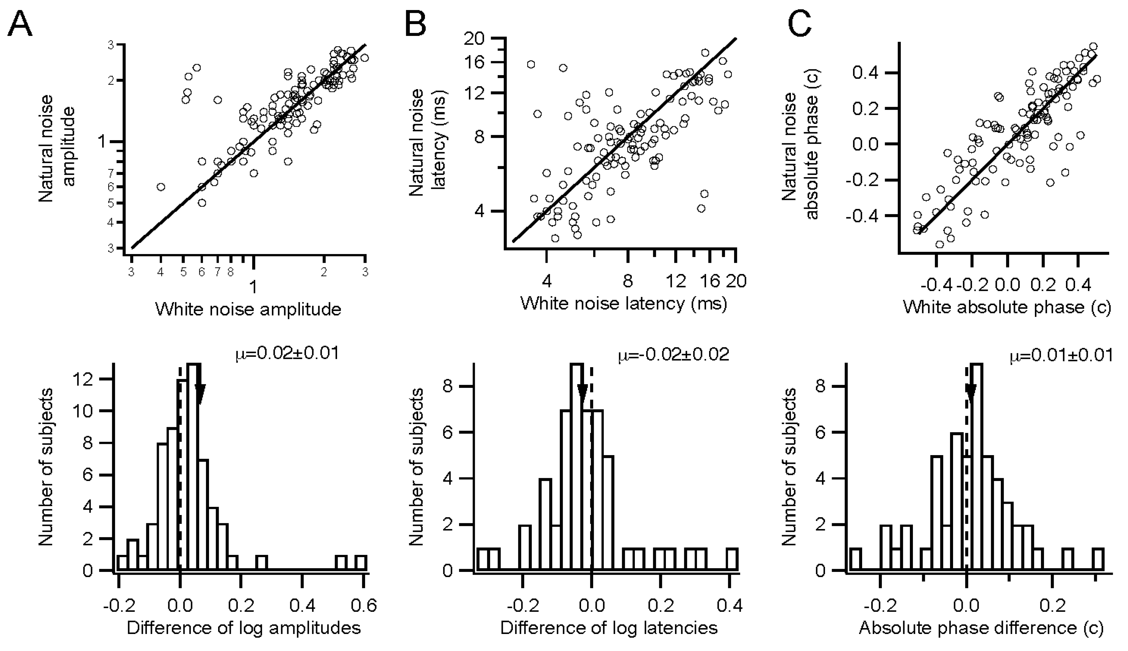
Retinal function can be evaluated under somewhat more natural conditions than are standard. Stimuli can have natural temporal statistics, with lower contrast. Sampling times may be relatively long, in order to overcome low stimulus contrasts. Temporally natural stimuli did not require much longer sampling times than white stimuli, on the other hand.
More natural stimuli should let the clinician observe retinal function in a more relevant context. A considerable literature suggests that slowing down the conventional 75 Hz temporally white stimulus permits observation of certain response components more clearly [
12,
13,
14]. Work remains to be done to clearly show that these components are clinically useful, however [
15]. Low contrast stimuli have been used in several studies [
16,
17,
18], though data are limited. Mydriasis is typically the most bothersome part of the experience for the patient, and that may be dispensable as well [
19,
20].
3.2. Release from Fixation
We examined whether patients might be released from the standard fixation task during multifocal electroretinography. The evidence suggests that multifocal ERGs can be obtained in the presence of eye movements. Relaxing the requirements for fixation should be advantageous for many patients who have difficulty holding still and staring straight ahead. These advantages come with disadvantages. Many of these involve the lengthy computations needed. Analyses cannot be performed in times at all comparable to those available in the conventional system [
21]. Sampling time is also longer.
3.2.1. Analysis Time
Although kernel computations are far more complex, they can be completed, even with relatively slow hardware, in reasonable amounts of time for most clinical purposes. In addition, by using faster and especially multiple processors, analysis time should decrease dramatically. These are highly parallel problems that can be usefully treated with graphical processing units that have become relatively inexpensive.
3.2.2. Recording Time
Sampling times may remain relatively long, in order to overcome low stimulus contrasts and additional artifacts from eye movements. However, this is partly compensated by improved comfort for the patient. Watching a movie for tens of minutes may be a more pleasant experience for most patients than a few minutes of fixating on flashing patterns. We are gathering subjective data on how subjects feel about their testing experience.
3.2.3. Eye Movement Artifacts
Remarkably, the artifacts generated by eye movements do not drastically interfere with measurements of retinal responses. This is partly due to the fact that saccade frequency is low enough and saccade amplitudes are often small enough that a substantial portion of the recording time occurs while the eyes are only moving slowly. The artifacts generated by small saccades have durations shorter than the typical intersaccadic interval, so that retinal responses can be seen between saccades without artifacts present. Combining this fact with analysis techniques that remove artifacts from consideration permits extraction of accurate kernels [
22]. Brute force methods of discounting artifacts can be problematic [
11]. Our methods rely largely on median filtering of amplitudes, and especially on the reliance on phase that is not sensitive to artifacts.
3.2.4. Decorrelation
Eye movements help to decorrelate the stimulus across space and time from the point of view of any retinal location [
23,
24,
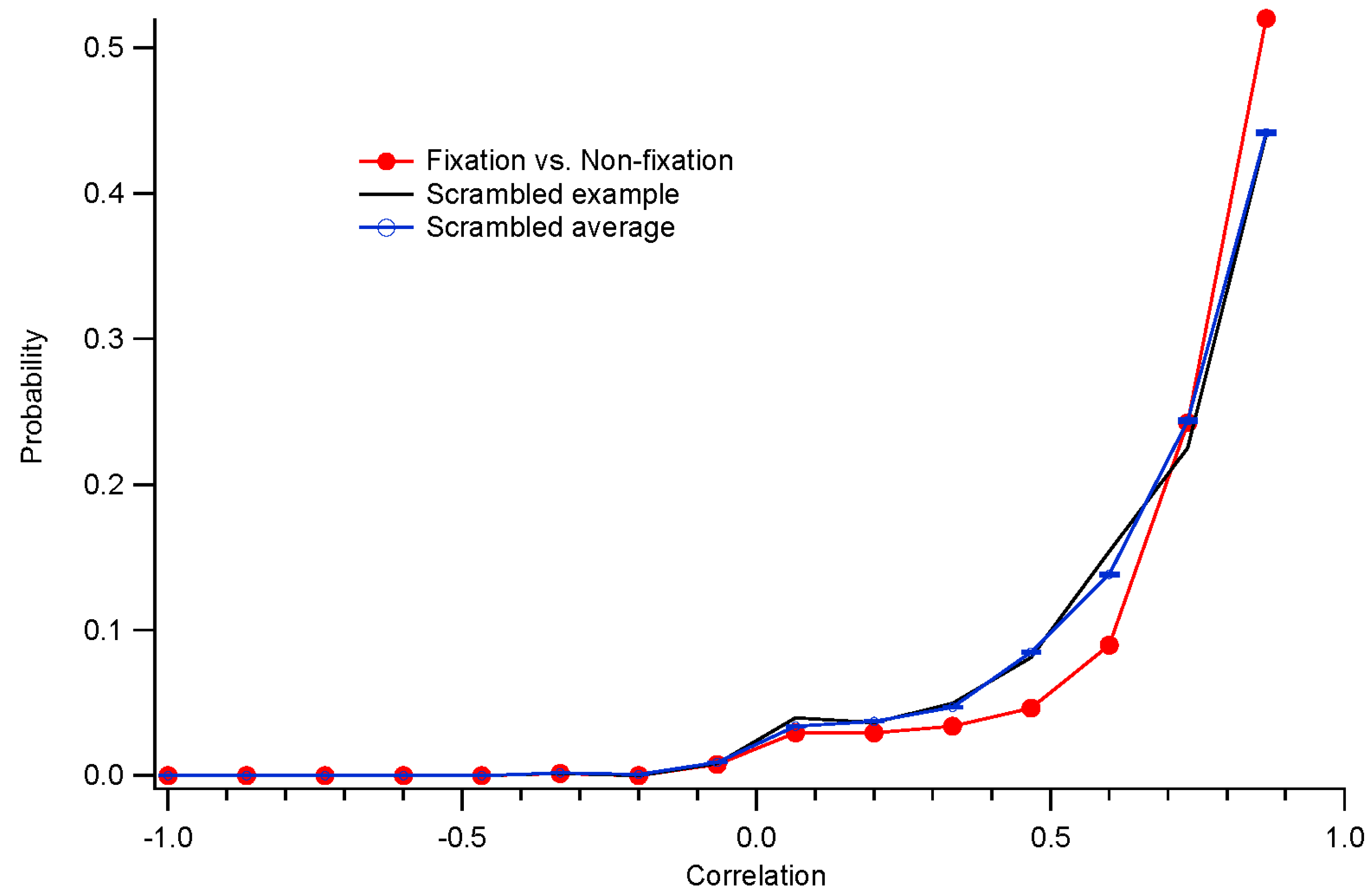
25]. The spatial decorrelation performed here is facilitated greatly by this fact. During fixation conditions, the spatial correlation matrix is highly singular, but becomes less so during non-fixation conditions.
3.3. Advantages and Disadvantages
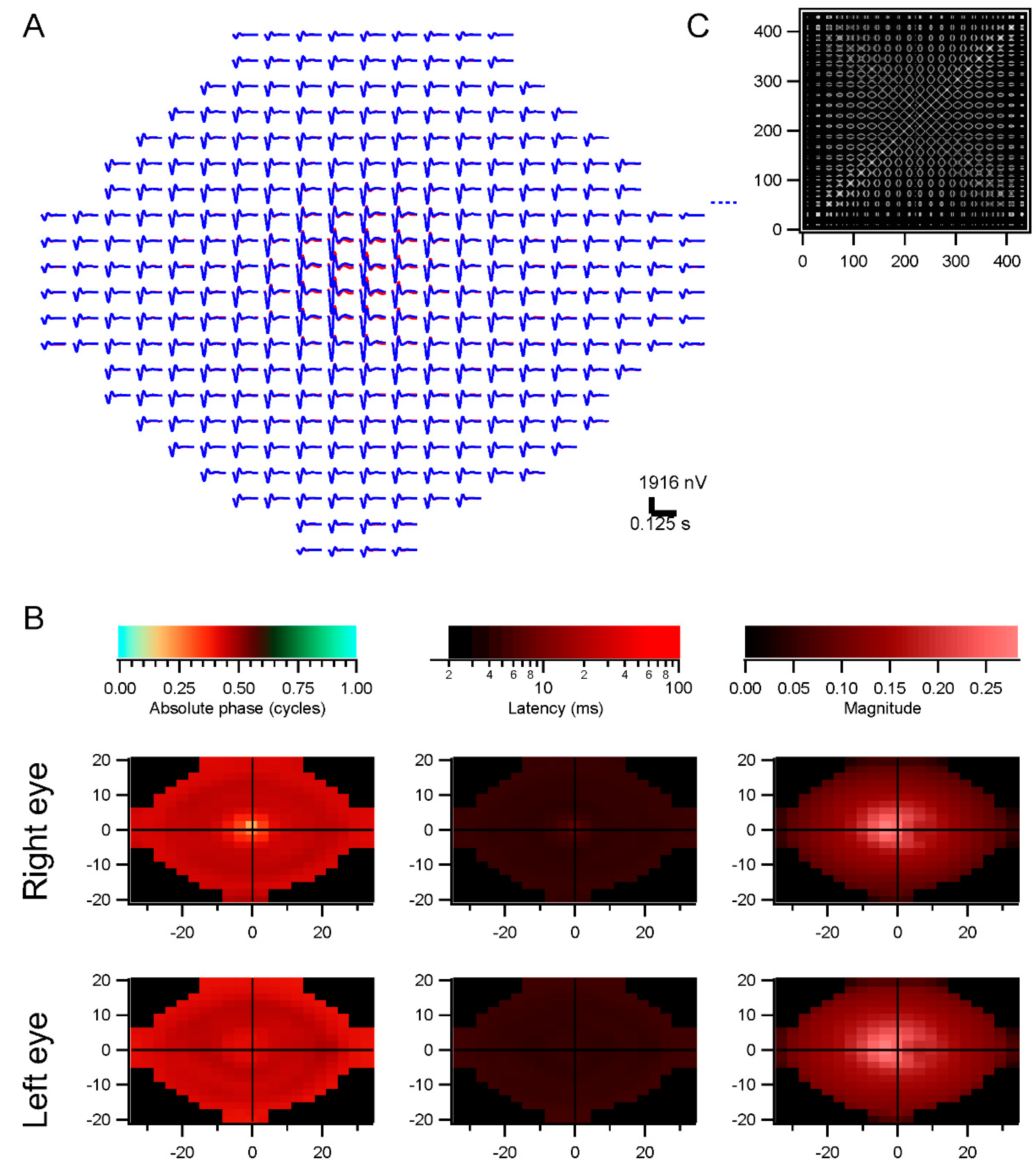
Among the flexible aspects of these methods, we can arbitrarily choose both the stimulus configuration and the analysis grid. For example, these can be customized to match features in a visual field, OCT, or fundus photo. The stimulus can be optimized to reveal pathologies at particular locations. The flexible methodology provides additional choices that can be seen as complicating clinical decision-making, but in many cases simplifies testing and makes it more efficient. For example, a common protocol is used for monitoring patients who have a long history of hydroxychloroquine use. Testing is conventionally done with a set of hexagonal stimulus elements that are then averaged across rings, to detect the typical pattern of bullseye maculopathy. By instead making the stimulus a small set of rings, more power is assigned to the stimulus, and the analysis is clearly simplified.
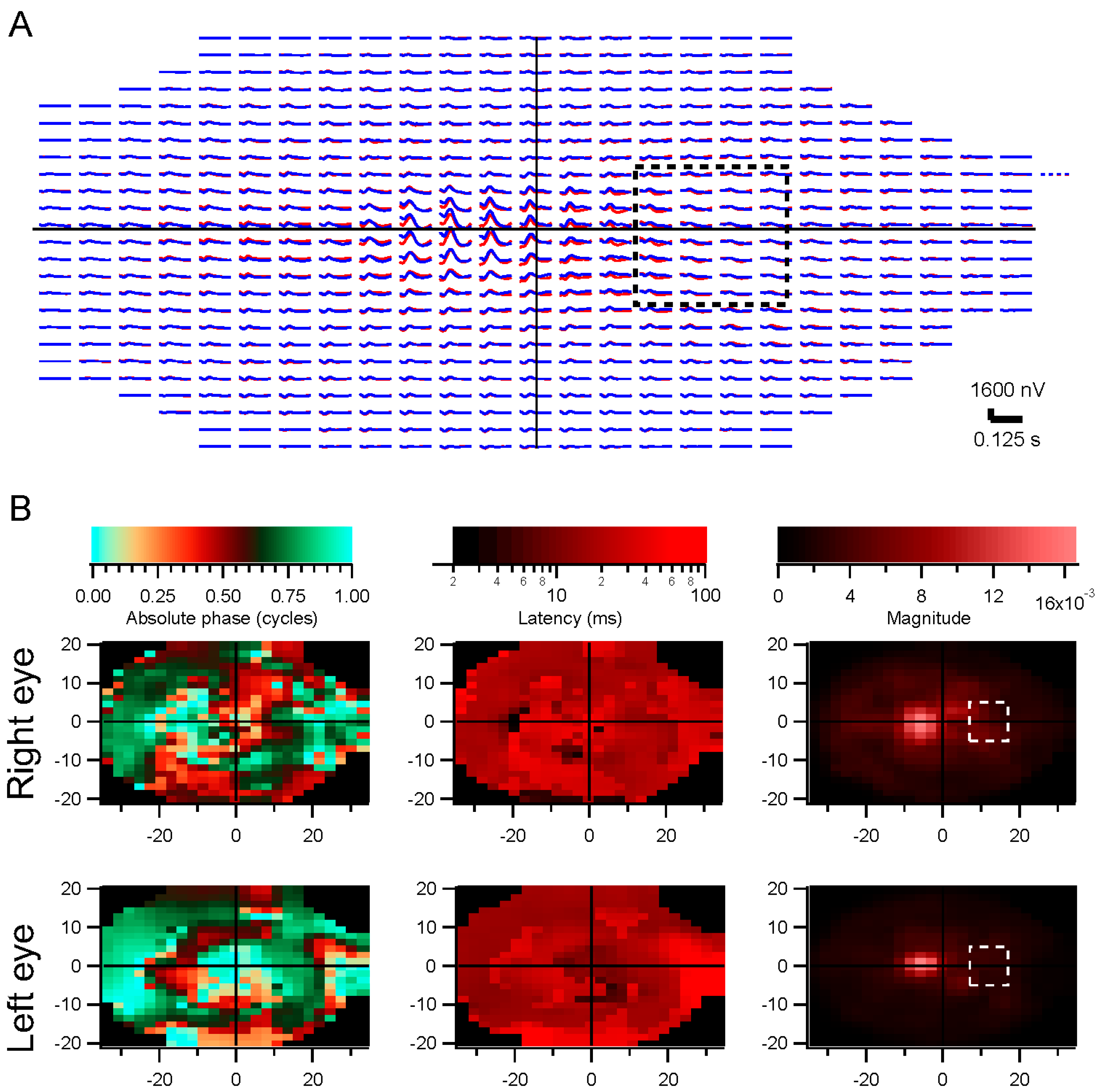
These methods have been used successfully with dozens of patients. One example of their utility comes from testing a patient with macular degeneration, who had some nystagmus and many fixational saccades during testing. The stimulus-based analysis did not yield usable results except in the periphery, but the retinocentric method produced clean trace arrays, showing a strong peak a few degrees above the nominal foveal center.
Testing can be made more patient-friendly. A high percentage of patients are photophobic. Reducing temporal contrast is one way of making the experience more comfortable. Most people find it difficult to fixate for long periods of time, so releasing them from the fixation task makes it possible to record under more relaxing conditions for lengthier sessions. Giving patients something to watch that captures their attention and interest should be an additional bonus. Children could watch cartoons, for example, that would help to distract them from the sometimes intimidating environment of the clinic. Head-free gaze tracking is available that enables relatively free viewing.
Retinocentric analyses provide a novel means to focus on the ultimate goal, locations on the retina rather than on the screen. They make it possible to explicitly permit eye movements while recording. In addition, fixational eye movements and breaks in fixation can be easily handled by measuring eye position and regenerating the stimulus in retinal coordinates.
The ISCEV standards for mfERG provide crucial guidelines for clinics to provide high quality, consistent reports [
3]. The modifications we describe here deviate significantly from the conventional techniques, unfortunately, and considerable work will need to be done to bring these methods up to those standards. In particular, the efficiency and reliability of the m-sequence technique must be approached, with the ability to obtain robust kernels in brief testing times.
3.4. Spatial Decorrelation
The conventional system empirically scales the stimulus elements from center to periphery in order to achieve approximately equal signal-to-noise values for the kernels across the retina. Response density is then computed by dividing each kernel’s raw magnitude by the area of the corresponding stimulus element. That process shows that response density peaks sharply at the fovea, correlated with cone density. However, this normalization can produce a spurious central peak when kernels are noisy. When performing a retinotopic analysis, the division by stimulus element area is replaced by normalizing by the stimulus correlations, such as via subtracting contributions from other retinal locations through the iterative decorrelation process. When using scaled stimuli, peripheral locations have stronger correlations with other locations than do central locations, so that their raw kernels are reduced.
The central kernels are typically not as strong as expected with our methods. This may be due to imperfect decorrelation, since the large stimulus elements we use do not isolate the fovea, so central responses are contaminated by those outside the fovea.
The phases of the stimulus correlations could be important, for example in situations where eye movements create systematic movements across the retina, or if the stimuli themselves move systematically as in natural movies. The correlation phase captures how stimuli move from one retinal position to another. Those movements need to be discounted, so that, for instance, responses from one retinal region are not attributed as later responses from the part of the retina to which the stimulus evoking the responses moves.
How well the decorrelation works remains to be determined. The artificial scotoma experiments, along with clinical trials, will enable testing of these methods. In the presence of eye movements, stimuli are more decorrelated across a long span of testing time. That should further indicate how well the decorrelation, applied during fixation trials, matches the non-fixation results.
4. Material and Methods
4.1. Subjects
Full screen and/or multifocal ERGs were obtained from 68 healthy subjects. They were recruited by advertising and word-of-mouth. Geometric mean age was 28 years, range 14–81 years, 74% were women, 43% were African-American. Subjects provided written informed consent and assent after the procedures and potential consequences were explained in full. All procedures were approved by the Institutional Review Board of Georgia Regents/Augusta University Medical Center (611231-6, 1 June 2014), and complied with the Declaration of Helsinki.
4.2. Recording Preparation
Drops of Proparacaine HCl (0.5%), Tropicamide (1%), and Phenylephrine HCl (2.5%) were applied to each eye for anesthesia and mydriasis. Areas of skin where reference and ground electrodes would be placed were scrubbed with alcohol pads. Reference electrodes were clipped to the ear lobes, and a cup electrode was taped to the forehead as a ground. Skin electrodes were filled with conductive gel. DTL-Plus electrodes (Diagnosys LLC, Lowell, MA, USA) were carefully placed across each eye, avoiding lashes and situating the adhesive pads so that the fiber ran directly along each canthus. Subjects reported not feeling the electrodes in nearly every case, even after more than an hour.
A table with the stimulating monitor and a chin rest was positioned at a comfortable height, and the chin rest was adjusted to accommodate the subject’s head. A video camera with infrared illumination (Arrington Research 220, Scottsdale, AZ, USA) was focused on one eye. Settings were made to optimize capture of the pupil, and a calibration was performed with the Arrington software. Voltages scaled across the eye position range of the monitor were sent from the Arrington system to a digitizer (National Instruments NI-6323, Austin, TX, USA). Another calibration was performed using custom software in Igor Pro 6 (WaveMetrics, Lake Oswego, OR, USA) based on those voltage signals. Any time the experimenters suspected it might be needed, an additional calibration was performed. During recording, each trial was preceded by recording eye position until it stabilized as the subject fixated, and these records were used as slip corrections to compensate for small head position changes.
Electrode signals were led to a PsychLab (Cambridge, MA, USA) EEG8 amplifier. Typically, gain was 10,000×, and the amplifier filtered the raw signal between 1 and 200 Hz. No notch filter was used. The amplifier output was digitized by the same NI-6323 DAQ (National Instruments, Austin, TX, USA) simultaneously with the eye position signals.
4.3. Visual Stimulation
Subjects viewed stimuli on a Samsung (Ridgefield Park, NJ, USA) 2233RZ 120 Hz LCD monitor at a distance of 29 cm. The viewing area on the monitor subtended about 70° × 40°, and the maximum brightness was set to 200 cd/m
2. The stimuli took advantage of the aspect ratio of the screen, extending horizontally about 175% of the vertical extension. This monitor has excellent timing [
26]. The time when each frame was presented was stored for synchronization with the electrode signals.
Stimuli were drawn on the screen by code written in Igor Pro. A fixation target, consisting of a diagonal cross and a circle, was present either during the initial 500 ms, or throughout the 4 s trials. Each trial was preceded by early appearance of the fixation target and either a message on the screen or an audible tone alerting the subject to the onset of the trial, so that they would fixate, and slip correction data (see
Section 4.2) could be measured. The mean luminance of the screen was maintained constant at 100 cd/m
2. Subjects could request a break at any time during sequences of trials. Intertrial intervals were typically 4 s.
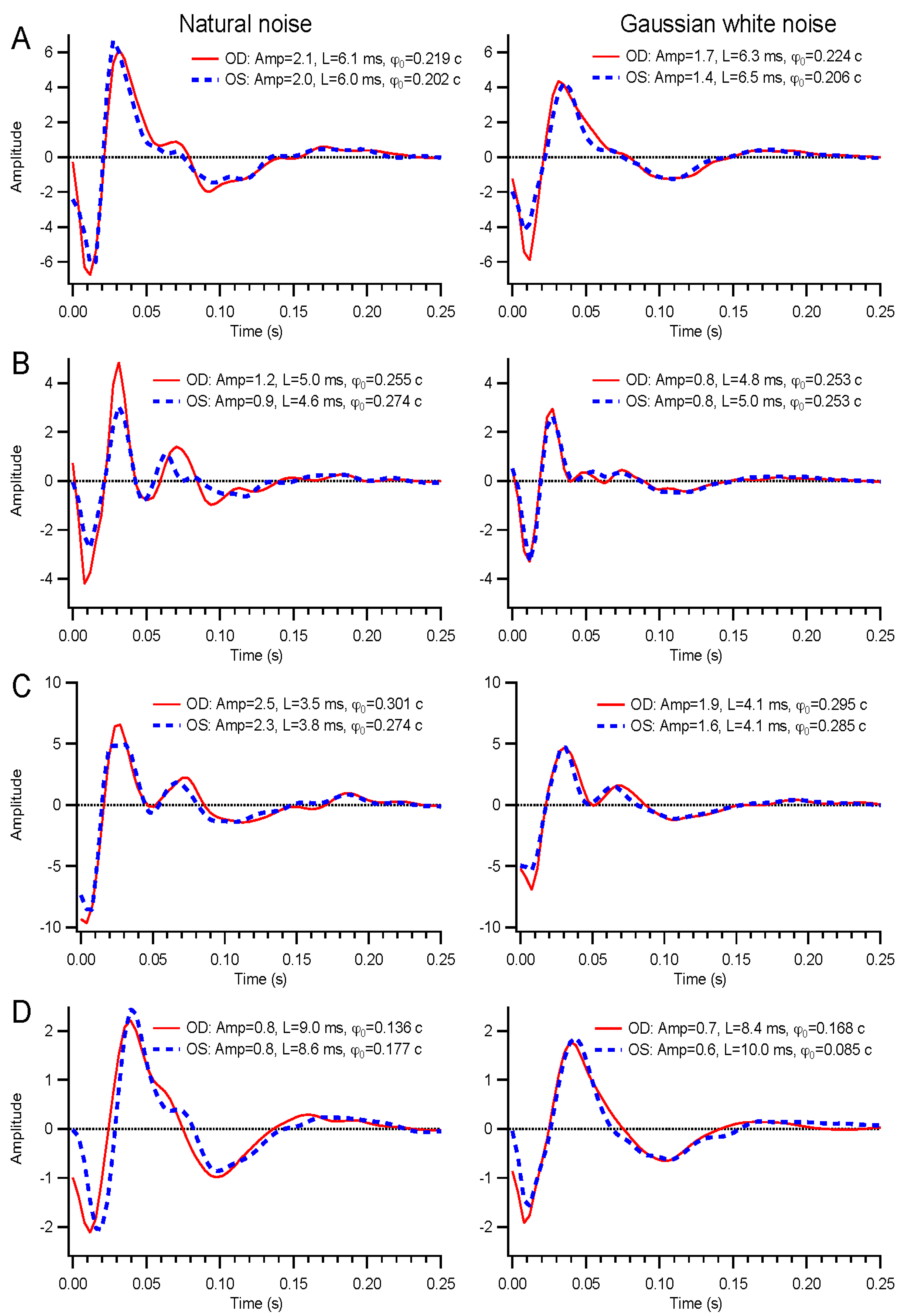
A wide range of temporal modulations could be applied to the stimuli. For this report, we describe results from binary white, Gaussian white, and natural noise modulations. Binary white stimuli had the luminance of each frame chosen from the minimum and maximum luminance levels based on a pseudorandom number. Gaussian white stimuli contain a continuous, normally-distributed set of luminance values chosen independently on each frame. Natural noise is also continuously distributed, but the luminance on each frame depends on the previous frame’s value, Ln = f(0.9Ln-1 + 0.1γ), where γ is a normally-distributed random variable with zero mean and standard deviation of 0.37, and the function f is a sigmoid that enhances contrast and bounds the luminance values between −1 and 1, to be subsequently rescaled to the range 0 to 200 cd/m2. The temporal contrast of the binary noise was 1, but the continuously distributed stimuli each had contrasts of about 0.29.
4.4. Experimental Protocols
We present results in this report from ERG testing with either full-screen, dartboard, or hexagonal patterns. Eye position was monitored in all cases with the Arrington pupil tracker. For some experiments, subjects were instructed to fixate throughout the run. Other experiments were designed to examine the effects of releasing the subject from the fixation task. For direct comparison, randomly interleaved trials were presented under the fixation and non-fixation conditions. Subjects were instructed to maintain fixation when the fixation target was present, but to move their eyes on trials where the target disappeared after 500 ms. Short lines of text (excerpts from Laozi, Lewis Carroll, Langston Hughes, Sean Singer, Maya Angelou, and Tagore) positioned randomly on the screen were provided on non-fixation trials so that subjects had something to look at and move their eyes across.
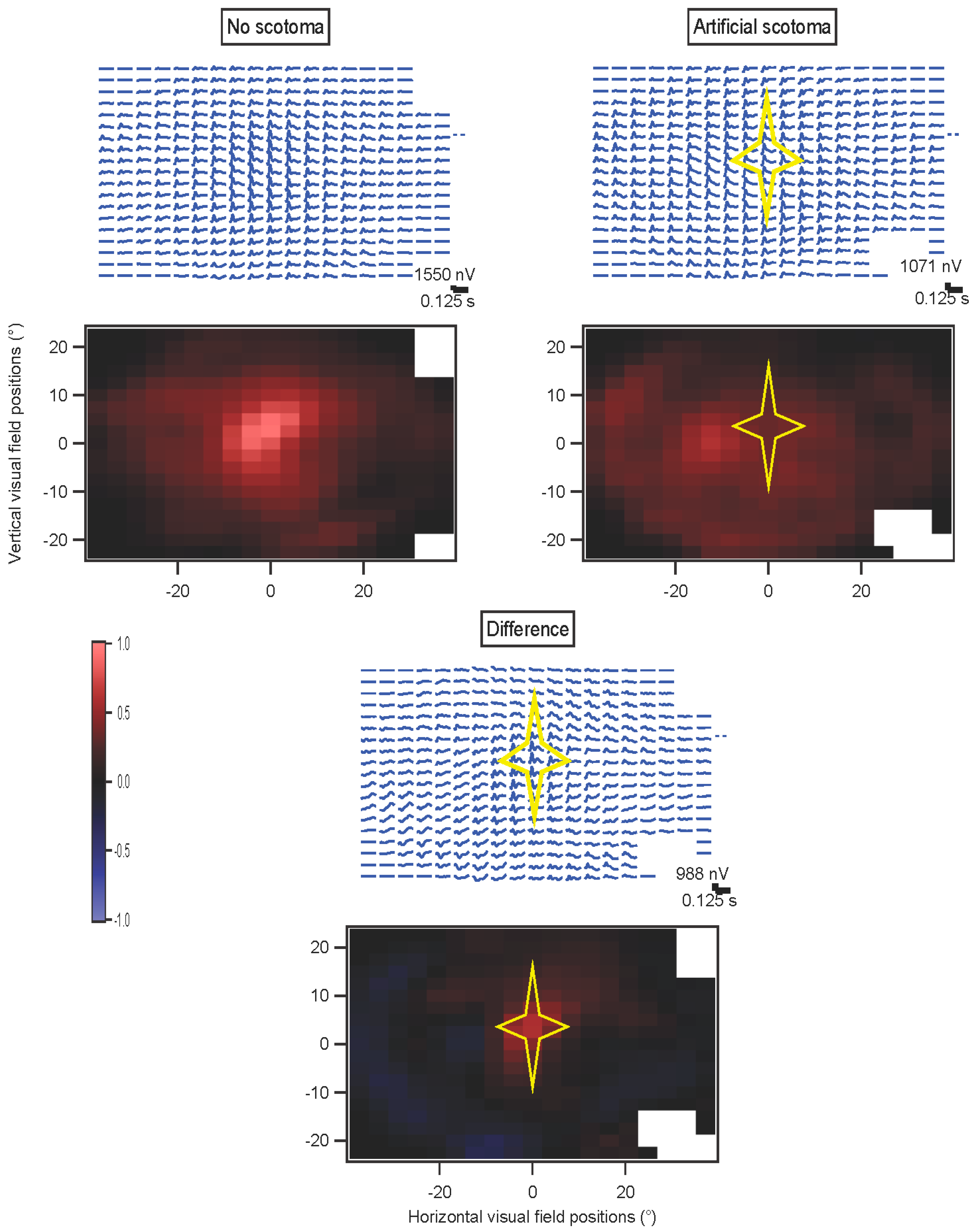
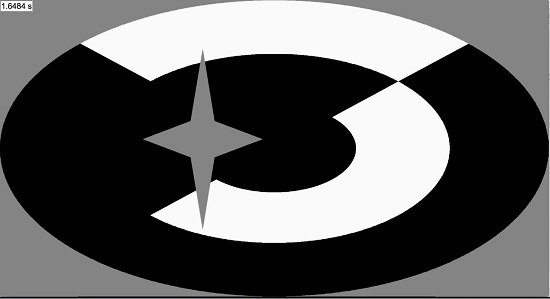
In some experiments, a star-shaped portion of the screen was drawn in gray over the multifocal stimulus. This artificial scotoma was shifted with the eyes, to maintain its retinal position
(Movie S2, Supplementary Materials). These experiments were performed using four randomly interleaved conditions: fixation trials with no scotoma; fixation trials with scotoma; non-fixation trials without scotoma; and non-fixation trials with scotoma. Results for each of the four conditions were extracted separately. The kernels for the scotoma conditions were then subtracted from the kernels for the non-scotoma conditions. A comparison was computed for the non-fixation conditions, where an index (difference divided by sum) comparing the non-scotoma and scotoma amplitudes was plotted to provide a statistical measure of the effects of the scotoma.
Because of hardware and software limitations, presentation rates above 60 Hz could only be achieved for multifocal stimuli with a limited number of elements. This was especially true when artificial scotoma position was updated and redrawn in real time, which slowed processing.
Horizontal positions were corrected for the offsets of the two eyes. However, figures are shown with matching locations of the kernels, for clarity. Amplitudes have been scaled with these corrections.
For the experiments using natural temporal stimuli, only full-screen stimuli were used, to focus on the temporal issues, and inversely for the multifocal stimuli, only binary white temporal modulations were used, in order to focus on the spatial issues.
4.5. Wavelet Correlations
Responses were correlated with stimuli via the wavelet correlation method [
9]. The goal of the analysis is to estimate the kernels that relate stimuli to responses. The first-order kernel is simply the response divided by the stimulus, in the frequency domain. Transforming the frequency domain kernel to the time domain yields the more familiar version of the kernel, also known as the impulse response function.
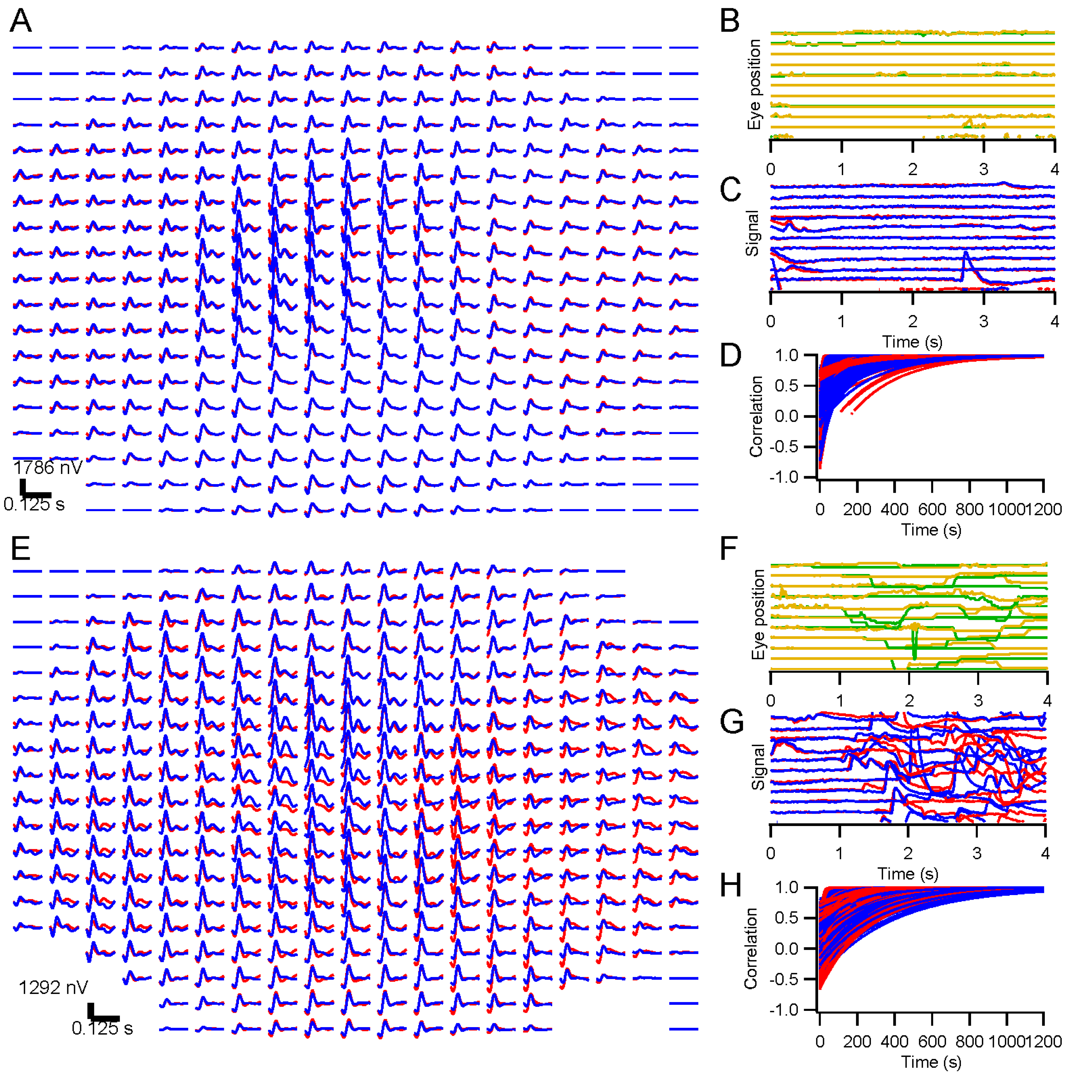
Each 4 s record of the stimulus luminance and electrode voltage was represented in the time-temporal frequency domain via a complex continuous Morlet wavelet transform. This representation provided a detailed view of amplitude and phase of the signals at 2048 time samples over 37 temporal frequencies ranging from 0.25 to 150 Hz.
The stimulus wavelet was filtered to remove low contrasts (below 1% of the average contrast across all frequencies and times). The response wavelet was then divided by the stimulus wavelet, to provide an estimate of the kernel at each time sample. A key step was then imposed: at each frequency, the amplitude of the kernel estimate was median filtered across time to remove artifacts. The median filter looked over ±1 s around each time point, and if the amplitude deviated from the median over those 2 s by more than the standard deviation of the amplitude over the whole 4 s trial, the amplitude was instead set to the median. This median filtering was iterated until its effect was less than 5% of the maximum amplitude. Artifacts, including those evoked by eye movements, were greatly discounted by this procedure. Note that this median filtering was only applied to the amplitudes. Crucially, phase was unaffected, other than reducing the effects of artifactual phase values. This is different from median filtering in the time domain.
The filtered amplitude was then recombined with the phase of the kernel estimate (kernel phase is response phase minus stimulus phase), and for each frequency the average over the time samples was computed in the complex plane. Only times within the “cone of influence” were considered, omitting times near the beginning and end of the trial for low frequencies. The cone of influence included points where the wavelet transform provided amplitudes to sinusoidal tests within two standard deviations of the maximum amplitude at that frequency.
The kernel estimate was then interpolated to a function of 513 frequencies ranging from 0 to 128 Hz, avoiding extrapolation. Kernel estimates were averaged across trials. The same process was applied to derive control kernels, using a stimulus rotated in time by a random amount between 1.5 and 2.5 s to disrupt real correlations.
Note that all of these calculations are performed in the frequency domain. Kernels were only transformed to the time domain for illustration purposes.
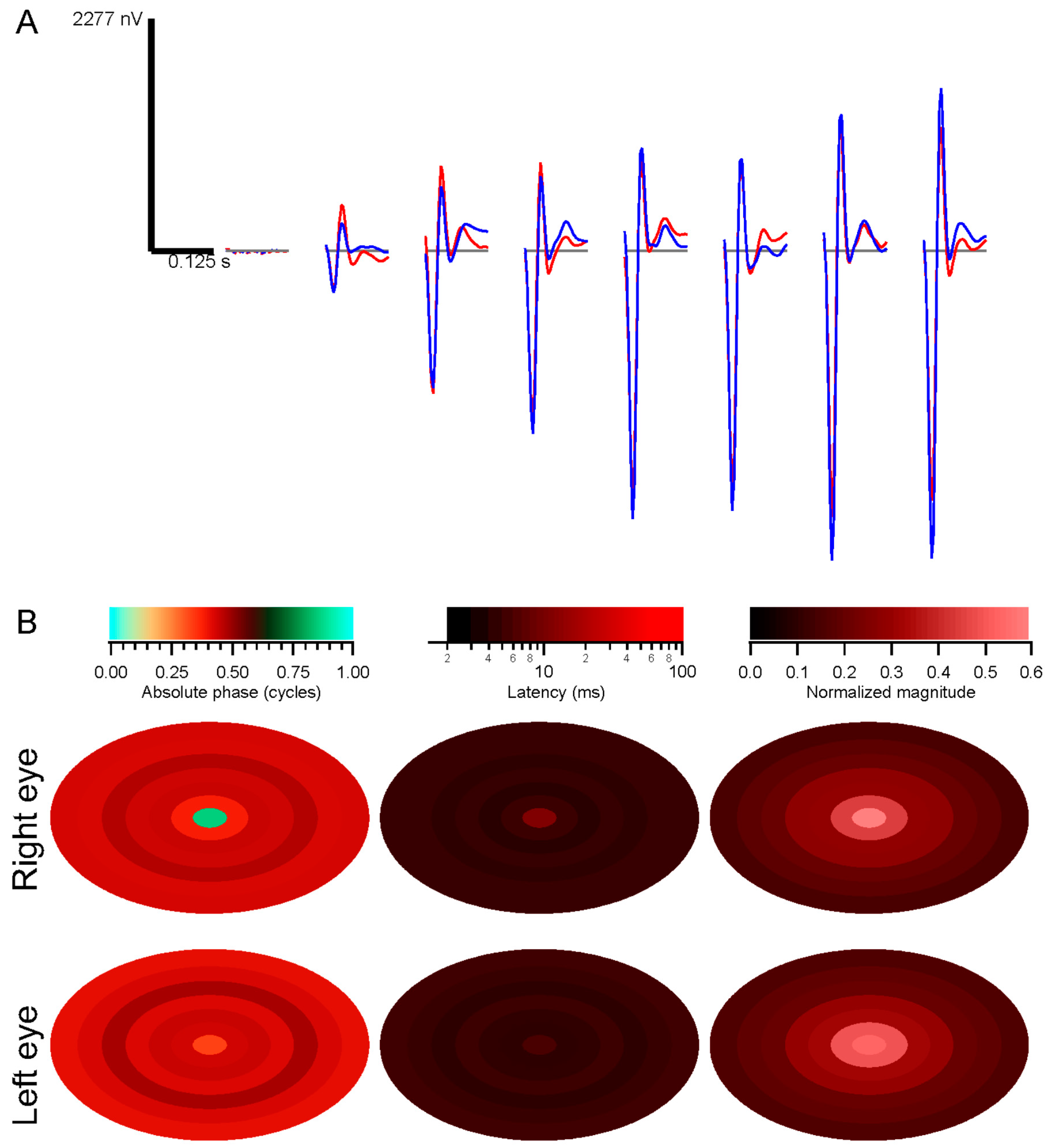
Kernel characteristics were quantified primarily with three parameters. Amplitude is taken as the root-mean-square value of the impulse response over the first 500 ms. This is equivalent to the total power in the frequency domain [
27]. Timing was measured with a linear regression of phase
vs. frequency [
28]. The slope is the latency, and the intercept is called absolute phase, measured in cycles. Absolute phase corresponds to the shape of the kernel. Absolute phase of 0 means a sustained response, with a unimodal shape. Absolute phase values just less than 0 arise from kernels with an initial positive mode followed by a smaller negative mode. A small initial negative mode followed by a larger positive mode produces a slightly positive absolute phase: this is the most common shape of photopic ERG kernels (
i.e., a-wave followed by b-wave).
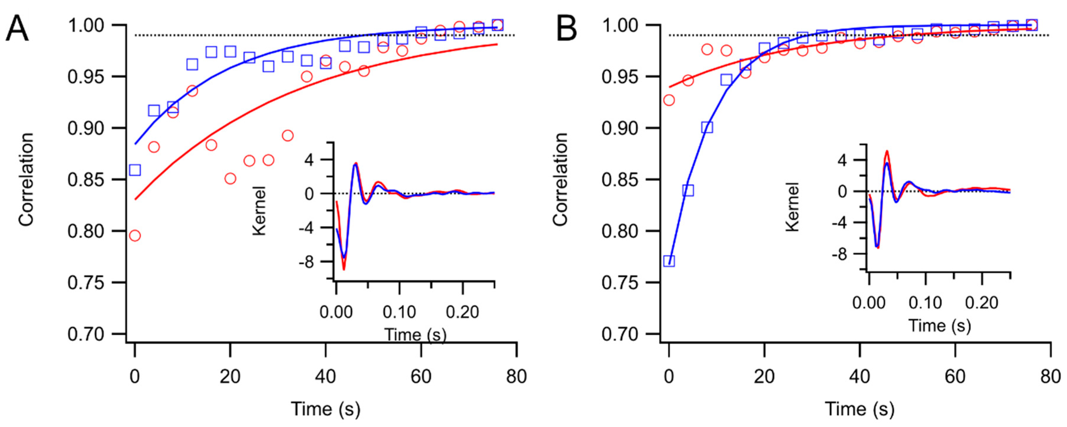
Kernels accumulated after each trial were stored. These were compared to the “final” kernel after the last trial by correlating the impulse response functions. The correlation coefficients approach 1 asymptotically by design. Two measures of convergence rate were obtained: the time constant for an exponential fit, and the first time at which the correlation coefficient exceeded 0.99 and did not later fall below that level.
4.6. Retinotopic Analyses and Spatial Decorrelation
For the multifocal experiments, stimuli were discretized in space across the retina by choosing a grid covering an area larger than the most strongly stimulated portion of the retina. For each stimulus frame, the screen stimulus was shifted based on the eye position record, and the mean luminance in each retinal grid element was taken as the luminance value for that frame. The sizes of the chosen grid elements were smaller than the sizes of the stimulus elements, with at least 4–5 grid elements for each stimulus element, typically; however, contrast tended to be lower for grid elements located along stimulus element borders at central gaze.
The grid-based retinotopic stimuli were correlated with the responses from each eye, via the wavelet correlation method (Subsection 4.5; [
9]). The kernels estimated in this way contain information not only about retinal function at the corresponding grid points, however, but are influenced by retinal function at other locations where the stimulus was correlated with the stimulus at the home position. These correlations need to be removed in order to isolate the contribution to each kernel only from its own retinal location. Decorrelation was performed as follows.
We make the assumption that the global ERG signal (
r) arises from a uniform linear combination of the local ERG signals:
where
ki are the kernels and
si the stimuli across locations
i, and
is the convolution operator. In the frequency domain this becomes
where the upper case indicates Fourier transforms of
r,
k, and
s (these are functions of time, so their Fourier transforms are functions of temporal frequency).
Correlating the response with the stimulus at a location
j, which is equivalent to multiplying both sides of Equation (2) by
, gives
where the
indicates complex conjugation. This can be written as
where
(superscripts are used to index over iterations below, so this is for the 0-th iteration) is the vector of kernel estimates prior to decorrelation,
K is the vector of decorrelated kernel estimates, and
C is an asymmetric correlation matrix
We can thus solve for the decorrelated kernels:
We compute the kernel estimates first as
, while compiling the stimulus correlation matrix
C. We could then invert the correlation matrix and compute the decorrelated kernels. In general, however, the correlation matrix is highly singular, and pseudoinverse methods we tried were not effective. We have used an iterative method to compute the solution for
K. Note that Equation (4) can be rewritten in a form that has intuitive appeal, as
because
One can see that the initial kernel estimate
K0 needs to be corrected by subtracting the unwanted contributions of other retinal locations. We compute these kernel estimates iteratively, so that for the n-th iteration.
until they converge,
, as α
n approaches 1 from below, for ε small. Convergence is not guaranteed. For example, a full-field stimulus would mean that all correlations were exactly 1, and obviously would not permit local kernels to be distinguished. The iterative computations tend to be unstable, and we implemented controls to reduce this instability. The detailed methods are available from the author.
These calculations are extremely slow, and for the purposes of most of the results in this report, we show simpler decorrelations. Instead of using Equation (6) with complex correlations, we divide
K0 by the real-valued instantaneous averaged stimulus correlations. Ignoring a phase like this only has minor effects in the current context, but becomes a problem when the stimulus contains coherent motion, as in natural movies, in addition to the coherent motion induced by smooth eye movements that are uncommon here [
29].

