1. Introduction
Achieving high dependability via replication of components and the reduction of design costs are typically conflicting goals [
1]. Traditional design strategies to improve a system’s fault tolerance use replication of hardware components that provide similar functions in redundancy configurations such as Triple Modular Redundancy [
2]. In general, replicated components mask component faults and provide recovery capabilities when faults compromise the delivery of function; accordingly, they are known as
homogeneous redundancies.
One possible way of improving dependability whilst reducing economic costs is the optimal use of hardware and software components that provide diverse functions [
3,
4]. In some scenarios, it is possible to use
heterogeneous redundancies consisting of components which, in addition to performing their primary intended design function, are also able to restore compatible functionalities of other components. This is often the case in highly networked scenarios,
i.e., systems where several replicas of system functions are distributed across the physical structure and connected through a network. For example, a train has replicated functions throughout its cars while a building has replicated functions throughout its floors and rooms.
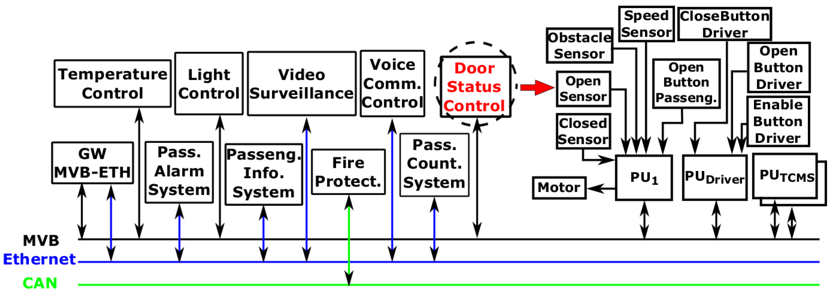
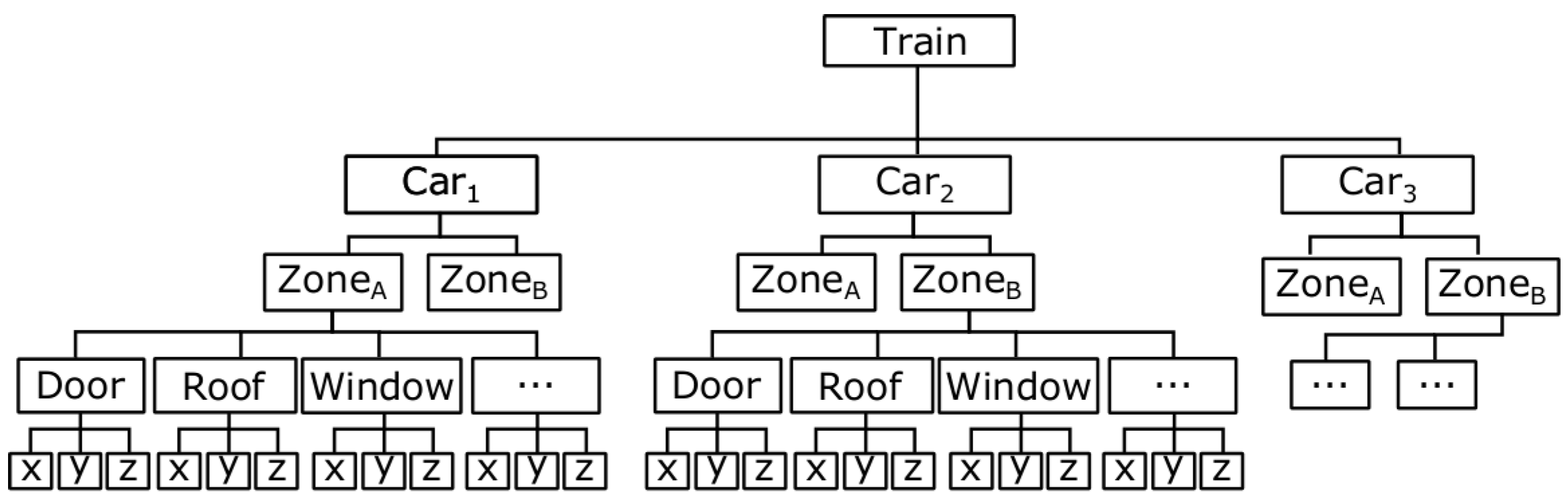
Figure 1 shows an example configuration of a single train car with its functions connected to different communication networks. Each function enclosed within a rectangle has its own components and this configuration is replicated for all the train cars.
For comfort functions, heterogeneous redundancies can be used freely, but for safety-critical systems, it is necessary to evaluate the effect of heterogeneous redundancies on dependability. In this paper, we focus precisely on this issue. System dependability is a term that encompasses a range of attributes which include safety, reliability, availability, maintainability, and security [
5]. We consider safety and reliability while maintainability and security aspects are outside of the scope of this paper. A common assumption made in dependability analysis is the ideal nature of health monitoring mechanisms ([
6,
7,
8,
9]). This assumption may lead the designer to adopt optimistic decisions which may prove to be inadequately safe. In this paper, we move away from this assumption to evaluate the influence of imperfections of fault detection, reconfiguration and communication implementations on system operation. We assume both hardware and software causes leading to omission, commission, timing and value faults [
5].
The analysis is facilitated by the recently proposed D3H2 (aDaptive Dependable Design for systems with Homogeneous and Heterogeneous redundancies) methodology [
3]. The aim of D3H2 is to identify heterogeneous redundancies; create architectures to use redundancies; and evaluate the influence of design decisions on dependability and cost. The approach provides the designer with decision support in the choice among different types of redundancy and reconfiguration strategies. For the dependability assessment, we use Component Dynamic Fault Trees (CDFTs)—a modular variation of Dynamic Fault Trees which improves the readability of complex models [
4]. In this paper, we extend CDFTs with capabilities for criticality and uncertainty assessment to enable the improved evaluation of the impact of components faults on the system and deal with non-exact failure data respectively.
In earlier work [
4], we applied the methodology to a simple case study. In this paper, we extend this work by: (a) applying the methodology to a safety-critical railway application; (b) moving beyond the assumption of ideal health monitoring configurations to address imperfections; and (c) extending the CDFT approach integrating uncertainty analysis and criticality assessment. In software controlled systems, it is not easy to determine a specific failure rate value of software components. This extension enables the specification of failure rate intervals instead of single values and can be used to evaluate their effect on the system failure probability distribution. Throughout the paper, we assume that components are non-repairable assets while diagnostics and maintenance strategies are beyond the scope of this paper.
The remainder of this paper is structured as follows.
Section 2 overviews related work.
Section 3 presents the D3H2 methodology, emphasizing dependability analysis and the new contributions of this paper.
Section 4 applies the D3H2 methodology to the door status control of a train car. Finally,
Section 5 draws conclusions and identifies further analyses.
2. Related Work
Heterogeneous redundancies can take many forms: design diversity [
10], analytical redundancies [
11], or redundancies arising from overlapped system functions [
3]. All these approaches share a common design goal: the reuse of system components to provide a compatible functionality. In our approach, we identify and exploit implicit diversity which may exist in an application to provide improved fault tolerance and reduce costs. Detailed knowledge and mathematical formulation of the system is needed to get analytical redundancy relations [
11]. However, the complexity of the mathematical formulation increases with the system size, and this has led us us to adopt a function-based viewpoint with qualitative attributes, instead of a formal mathematical specification approach (see also
SubSection 3.2).
The evaluation of the influence of design decisions on system dependability and cost is an ongoing research challenge. While many works have concentrated on addressing the influence of homogeneous redundancies on system dependability and cost (e.g., [
12,
13,
14,
15,
16]), approaches focusing on the evaluation of heterogeneous redundancies are scarce.
Shelton and Koopman used functional alternatives to compensate for component failures and assign utility values to system configurations evaluating their influence on the overall system utility [
6]. Wysocki and Debouk reused processing units to continue operating in the presence of software component failures [
7]. They perform availability and cost evaluations using Fault Trees and Monte Carlo simulations. Methodological support for characterizing an adaptation model while meeting availability-cost requirements was presented in [
8]. For each system component, its implicit redundancies and quality constraints are specified to determine compatible components. System configuration probabilities are analysed using Component Fault Trees and Markov chains.
From the reviewed approaches, the following conclusions are emphasized (the reader is referred to [
9] for an extended discussion): the identification of heterogeneous redundancies is performed as an
ad hoc task relying on the designer’s creativity; the failure behaviour of health monitoring implementations and heterogeneous redundancy concepts have not been addressed; and the dependability assessment of heterogeneous redundancies and health monitoring implementations requires an approach that accounts for time-dependent events.
Therefore, to exploit the potential of heterogeneous redundancies, we present a methodology which integrates: (a) systematic identification of heterogeneous redundancies; (b) construction of system architectures that include hardware, software and communication components and deploy redundancies by means of fault detection and reconfiguration implementations; and (c) systematic evaluation of the influence on dependability and cost of the designed system architectures.
3. D3H2 Methodology
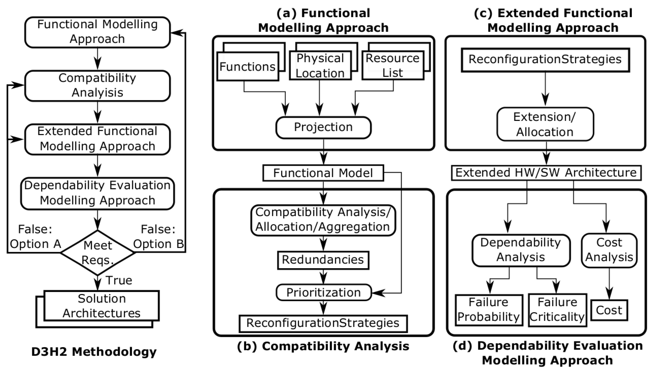
D3H2 integrates the modelling and analysis activities as shown in
Figure 2. Systems are specified as a set of interacting hardware, software, and communication resources, including their interfaces and provided functionality.
The main approaches integrated in the D3H2 methodology are listed below:
The
Functional Modelling Approach specifies the functional model including system functions, the physical location in which these functions are performed, and a necessary list of resources to develop these functions (see
SubSection 3.1).
The
Compatibility Analysis identifies compatible implementations (
i.e., redundancies) in the functional model. To use these compatibilities, it may be necessary to aggregate additional resources and perform the allocation activity for the new elements. Subsequently, reconfiguration strategies are defined including all implementations and their priorities (see
SubSection 3.2).
To use homogeneous and heterogeneous redundancies in highly networked scenarios, it is necessary to extend the functional model with fault detection and reconfiguration functions. To perform these functions, it also is necessary to allocate hardware/software (HW/SW) resources to the system functions. Accordingly, the extended HW/SW architecture is designed via an
Extended Functional Modelling Approach (see
SubSection 3.3).
Finally, the
Dependability Evaluation Modelling Approach predicts the dependability of the extended HW/SW architecture. The dependability and cost analyses allow designers to decide on design variants that achieve the best trade-offs between dependability and cost (see
SubSection 3.4).
Finally, the extended HW/SW architecture needs to be evaluated to verify if the initial requirements are met. If they are not satisfied there are two options: Option A takes the process to an earlier activity and iterates from there while Option B moves the design process back to its starting point so that design requirements are reconsidered. The reconsideration of design requirements from Option B results in the redesign of the functional model.
3.1. Functional Modelling Approach
The objective of the Functional Modelling Approach is the procedural consideration of system functions, resources, and the relations between them. The Functional Modelling Approach is inspired from the Structured Analysis and Design Technique [
17] and it has been designed to enable the systematic identification of heterogeneous redundancies and extraction of reconfiguration strategies.
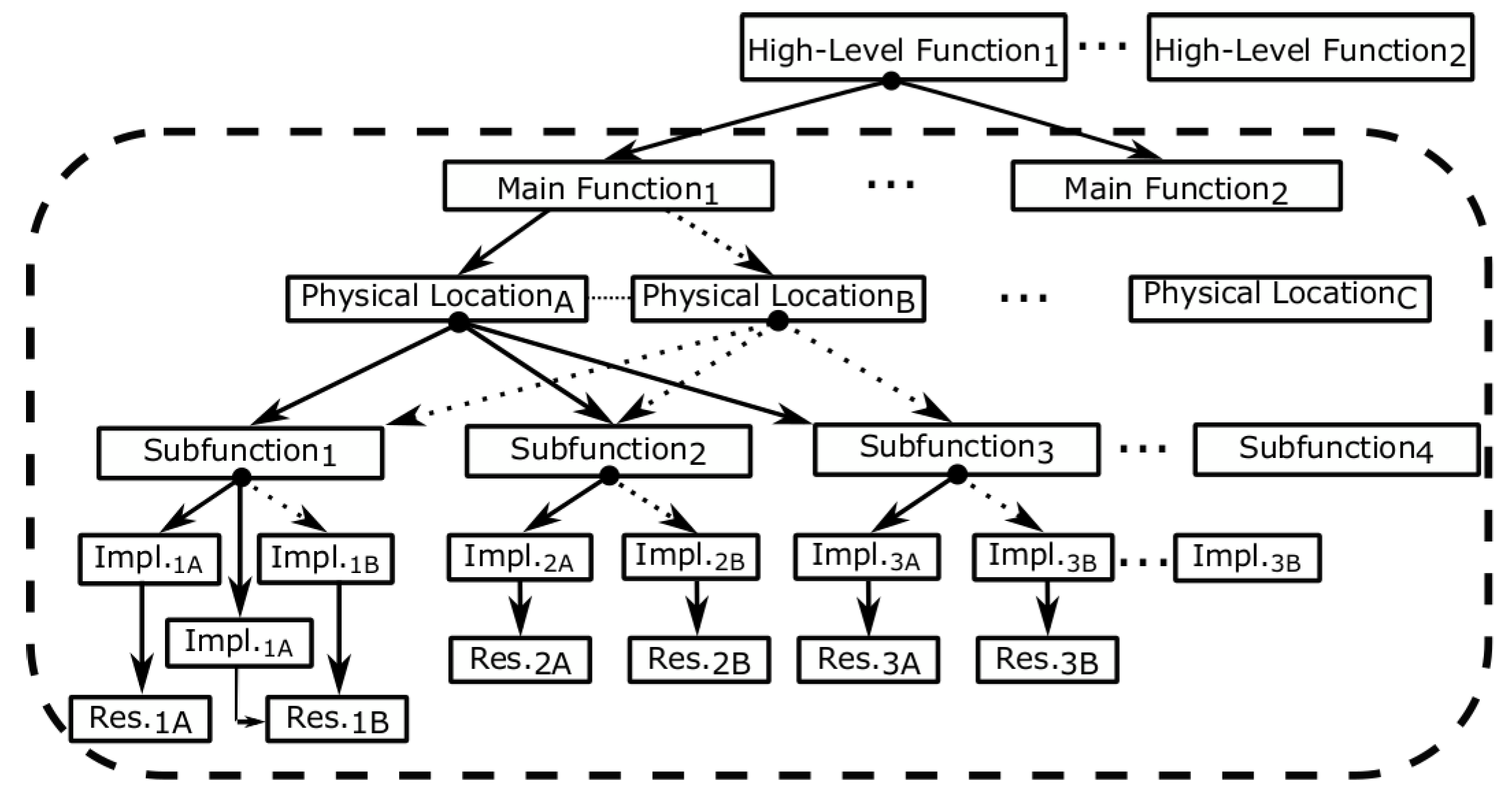
The Functional Modelling Approach specifies the functional operation of the system in a top-down manner based on tokens—starting from a set of high-level functions (e.g., different train operations: train operating properly, train stopped) tracing down to the necessary resources to perform these functions (
Figure 3).
A high level function consists of a set of Main Functions (MF), e.g., train operating properly = {traction system OK, signalling system OK, braking system OK,…}. These main functions are performed in possibly different Physical Locations (PLs), e.g., a single air conditioning control implementation may span a whole train car or each car compartment in a train car may have its own air conditioning control. Similarly, a main function consists of a set of subfunctions (SF), e.g., input, control and output subfunctions. A subfunction may have multiple implementations (#) to carry out the subfunction and these are ordered with respect to their priority. Each implementation requires a set of hardware, software and communication resources.
For simplicity, our token-based specification approach focuses on main functions and a first level of decomposition from main functions to subfunctions. However, note that the Functional Modelling Approach is extendible to
N functional levels. The full specification of a subfunction’s implementation of a generic main function is specified as follows:
To define consistently the physical location of system functions, a physical location map is defined for the physical structure.
Figure 4 shows the physical location map of an hypothetical train, where each car of the train is comprised of different compartments (Zone
A, Zone
B).
Based on the specification defined in Equation (
1),
Table 1 displays functional model examples of an existing railway train car, including typical main functions (
Figure 1), their physical location within the car (
Figure 4), and the necessary set of subfunctions and resources. For instance, the Fire Protection main function is performed in the compartment Zone
A of the Car
1 in the train. It is comprised of fire detection, fire protection control and alarm subfunctions, and the implementation of the fire detection subfunction is comprised of a fire detection sensor and a PU
FP processing unit (#1).
When designing a new system, the orientation of the Functional Modelling Approach focuses from system main functions toward resources (top-down). This design strategy requires planning and full understanding of the system so that an accurate overall picture of the system is obtained. Nonetheless, the drawback of this perspective is that it increases the development time and sometimes not everything is known at the beginning of a project (e.g., physical layout of the system). On the contrary, when addressing the redesign of an already existing system, a bottom-up first step is needed to obtain a functional model.
3.2. Compatibility Analysis
The Compatibility Analysis identifies heterogeneous redundancies based on tokens. Among system implementations defined in the functional model, there may exist two compatibility cases. Natural compatibility emerges automatically from compatible implementations carrying out the same subfunctions in compatible physical locations. Forced compatibility identifies available I/O implementations located at compatible physical locations automatically, and then evaluates whether they can fulfill additional subfunctions using engineering design knowledge.
We define
compatible physical locations according to the location of subfunctions (
Figure 4): (1) same physical location; (2) adjacent physical locations ([Train].[Car
1].Zone
A ↔ [Train].[Car
1].Zone
B); or (3) physical locations that span other PLs ([Train].[Car
1].[Zone
A] → [Train].[Car
1].[Zone
A].Door).
Therefore, we identify matching subfunctions and compatible physical locations in the functional model to determine if the analysed implementations are compatible or not. From
Table 1, the following heterogeneous redundancies are identified: alternative alarm signalling strategies #3↔#6 (
natural compatibility); contiguous compartment’s temperature sensor #10↔#12 (
natural compatibility); and an alternative alarm strategy using visual displays: #3→#9 and #6→#9 (
forced compatibilities).
Reconfiguration strategies integrate the functional model with redundancies. They define all possible realizations of the main function comprised of the necessary subfunctions and prioritized implementations. The prioritization is based on the weighted sum of [
3] functional degradation, failure probability and cost of the implementation. The functional degradation depends on the relative physical distance (applicable for heterogeneous redundancies arising from natural compatibilities). For heterogeneous redundancies arising from forced compatibilities, the designer’s knowledge is necessary.
As mentioned in
Section 2, analytical redundancies and heterogeneous redundancies have the same design objective. There are several approaches in the diagnostics and fault-tolerant control community focused on identifying analytic redundancies systematically (e.g., see [
11]). A number of approaches in this area evaluate if it is possible to provide the same service with a combination of remaining sensors,
i.e., if there exists an alternative analytic equation, which uses different set of variables (resources) to provide the same service. The identification of redundancies focuses on the relations among system equations and variables. That is, if there exists redundant information about the system structure (
i.e., if there are more equations than variables to be determined), there may also exist alternative ways to define a variable.
The exhaustive characterization and mathematical formulation of complex systems is not trivial, and, in some cases, it is infeasible. The identification of analytic redundancies is typically feasible at a subsystem level, but the complexity of the mathematical formulation increases dramatically at the system level. Additional complexity exists in highly networked scenarios where systems consist of many subsystems, which are all interconnected through a communication network. In general, the formal identification and categorisation of heterogeneous redundancies for complex systems is a challenging task. This is pronounced in the case of non-evident redundancies raised from forced compatibilities because there is no direct relationship between them.
3.3. Extended Functional Modelling Approach
The Extended Functional Modelling Approach augments the functional model by adding
health management functions and implementations;
fault detection to detect the incorrect operation of an implementation; and
reconfiguration to recover from implementation failures. We have defined the following mechanisms and protocols for fault detection and reconfiguration subfunctions:
Fault detection (FD): each subfunction has an associated fault detection subfunction (FD_SF). The FD_SF is located at the destination processing unit where the information of the source processing unit is used to detect communication omission failures directly.
Reconfiguration (R): each subfunction has its own reconfiguration subfunction (R_SF), which receives fault detection (FD_SF) signals and sends reconfiguration signals to subfunction implementations.
Fault detection of the reconfiguration (FD_R): each reconfiguration implementation (R_SF) has its own fault detection mechanism (FD_R_SF) implemented in keepalive configuration. Each R_SF implementation sends keepalive signals to all their FD_R_SF implementations to indicate that it is operating. In the absence of a keepalive signal during a time-slot, an R_SF implementation is assumed to be failed. When this happens, the FD_R_SF implementation sends an activation signal to the available R_SF implementation with the highest priority.
Communication is considered at resource level.
There does not exist a uniquely valid solution when allocating health management implementations (e.g., [
19]). The adopted decisions predefine the behaviour of health management mechanisms so that it is possible to design and evaluate extended HW/SW architectures systematically (see [
9] for further discussion).
Since fault detection and reconfiguration are subfunctions of a given main function, they are also modelled using
tokens (FD_SF, R_SF, FD_R_SF). Accordingly, it is possible to analyse alternative fault detection and reconfiguration strategies (see
Section 4,
Figure 8 for an example).
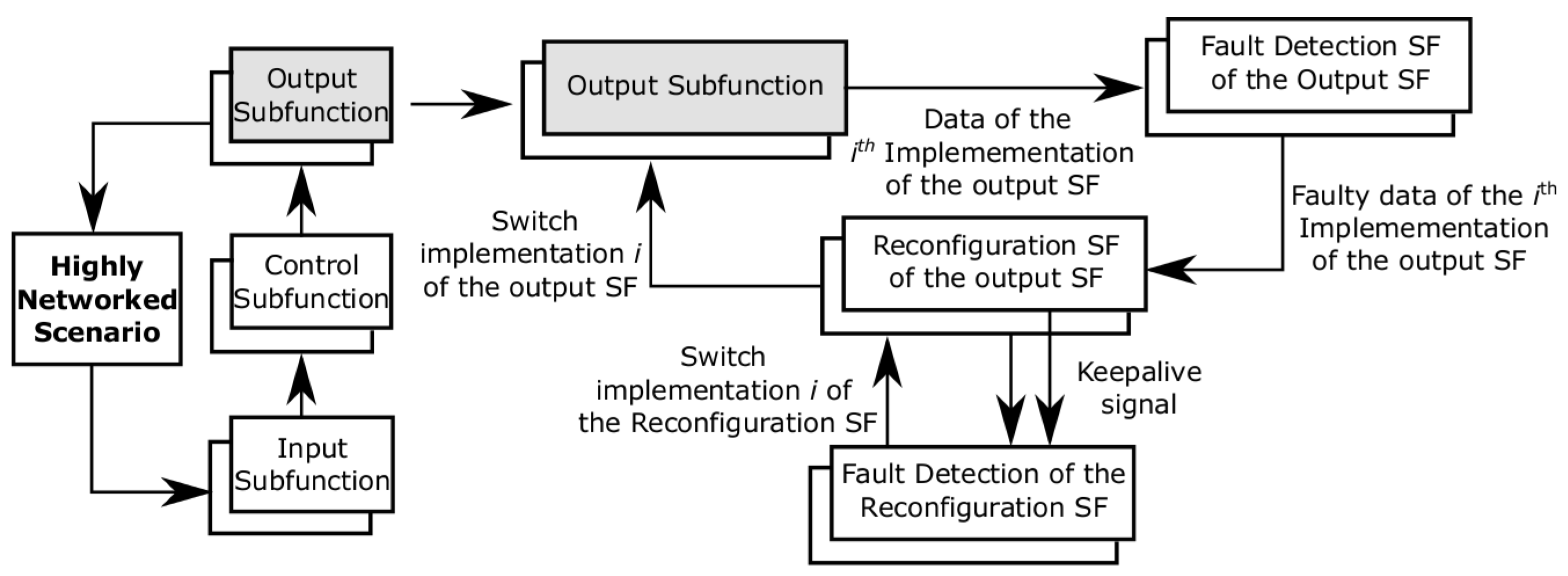
Figure 5 describes the closed-loop operation of a system deployed in a highly networked scenario including input, control and output subfunctions. The operation of the extended HW/SW architecture is described for the output subfunction with redundancies. Overlapped rectangles describe alternative implementations for the same subfunction.
Reconfiguration strategies are allocated at design-time in different processing units for the runtime reconfiguration of implementations. Each unit needs a wrapper that ensures the interchangeability between compatible implementations and a reconfiguration mechanism to redirect its information. Furthermore, the units with FD_R_SF implementations require monitoring
keepalive signals to control the correct operation of the active R_SF implementation (see [
4] for implementation details).
Depending on the allocation of each subfunction, the extended HW/SW architecture can deal with multiple simultaneous subfunction failures. For instance, if the reconfiguration implementations of subfunctions are distributed in different units, the independent and simultaneous reconfiguration of system functions is possible—so long as the communication does not fail. However, if they are allocated in the same processing unit, this would add bottlenecks to the design and could limit the number of subfunctions that can be reconfigured simultaneously. All these design decisions are evaluated with the Dependability Evaluation Modelling Approach in
SubSection 3.4.
The adopted design decisions are dependent on the assumed failure model. However, it is possible to include other fault-tolerance implementations such as roll-back strategies to recover from reconfiguration failures instead of using
keepalive implementations [
5]. The adoption of this strategy would require redesigning the extended HW/SW architecture and then analysing its effect on the Dependability Evaluation Modelling Approach.
3.4. Dependability Evaluation Modelling Approach
The Dependability Evaluation Modelling Approach evaluates the dependability of extended architectures through the systematic failure modelling of the system including all the possible failure scenarios [
4].
3.4.1. Preliminaries on Component Dynamic Fault Trees
In order to model the failure behaviour of the extended architectures, we need a dependability analysis approach that integrates the following characteristics:
Modular specification to improve clarity, maintainability, and traceability to the design architecture. Embed the failure logic of a set of events or components and (re)use it where needed.
Temporal logic to capture the system failure logic accounting for time-ordered events.
Specification of any cumulative distribution function of failure events.
Specification of repeated basic events, subsystems, or components.
Specification of NOT gates to address the influence of functional events.
The integration of classical Fault Trees with a compositional specification has been addressed in Component Fault Trees (CFT) [
20]. HiP-HOPS (Hierarchically Performed Hazard Origin and Propagation Studies) has a similar concept of compositional specification using annotations on the design architecture that can be used not only for safety analysis but also for design optimisation and requirements allocation [
21].
Dynamic Fault Tree (DFT) approaches extended classical Fault Trees with temporal gates [
22]. DFT implementations focus on simulation techniques to model failure events with any distribution function (e.g., Radyban [
23], RAATSS [
24]) or transformations into other stochastic formalisms (e.g, transformation into Generalised Stochastic Petri Nets [
25]). Boolean Driven Markov Processes (BDMP) combine mathematical properties of Markov processes with Fault Tree logic which result in a flexible dynamic specification logic [
26]. However, the Markovian assumption may be limiting for some systems.
There are also models that are both dynamic and compositional. Existing approaches such as State-Event Fault Trees (SEFT) [
27] and Generalized Fault Trees (GFT) [
28] define a high-level modular failure specification logic which must be transformed into a more fundamental dependability analysis formalism. The transformation results in a flat state-based system model. For instance, SEFTs are transformed into Deterministic and Stochastic Petri Nets [
27] and GFTs are transformed into Stochastic Well-Formed Nets [
28].
The Component Dynamic Fault Tree (CDFT) is suitable for modelling extended HW/SW architectures [
4].
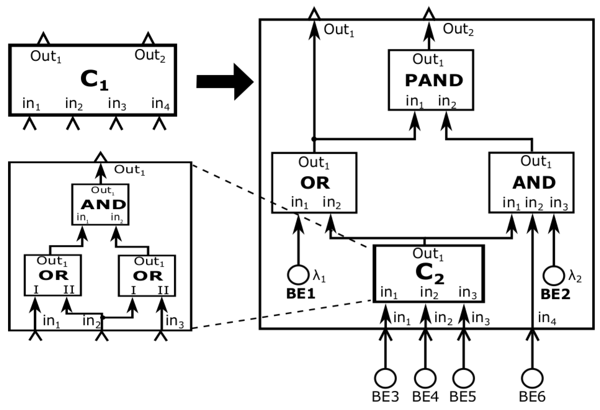
Figure 6 shows a CDFT example with repeated components (C
2) and CDFT gates. Each component (C
1, C
2) may have gates, basic events and/or other components as inputs. Each basic event (BE
1, …, BE
6) is specified according to its cumulative distribution function and its failure rates.
Inspired from the definition of Component Fault Trees [
20], a CDFT is defined as follows [
18]:
Definition 1. Component Dynamic Fault Tree: the Component Dynamic Fault Tree model, CDFT, is a 4-tuple
where:
N is the set of
Nodes, which are partitioned into a set of: internal events
, input ports
and output ports
;
. For instance, for the CDFT model depicted in
Figure 6, considering C
1:
,
,
.
G is the set of
Gates, where each gate
is described by: one output port
; one or more input ports
; a dynamic function which links inputs with outputs according to static (AND, OR, KooN) and/or dynamic (PAND) Fault Tree gates. As displayed in
Table 2, the behaviour of the CDFT gates are defined according to its input events (A, B), which can be extended to an arbitrary number of input events.
is a set of
Sub-Components, where each subcomponent
is described by: one or more output ports
; one or more input ports
; and a mapping to another CDFT component’s failure logic. For instance, for the CDFT model depicted in
Figure 6, SC=C
2:
,
mapping:
.
E is a set of directed Edges ((Nintern ∪ Nin ∪ G.OUT ∪ SC.OUT) × (Nout ∪ G.IN ∪ SC.IN)), where G.OUT is the set of all outputs of all gates; G.IN is the set of all inputs of all gates; SC.OUT is the set of all outputs of all sub-components; and SC.IN is the set of all inputs of all sub-components.
For the quantitative evaluation of CDFTs, Monte Carlo simulations are performed on the system’s failure evaluation algorithm in order to estimate the failure probability. Namely, for each execution, first the random time to failure of basic events is calculated according to their cumulative distribution function via the inverse transform sampling method [
29]. Let
F be a cumulative distribution function,
r be a random variable drawn from the uniform distribution
, and
the time to failure of the event. Then, the inverse sampling method applies the relation
to draw the time to failure according to the cumulative distribution function. Accordingly, a basic event has occurred (
i.e., signifies fault) when the
is smaller than the mission time. Connected gates and components use this information to determine their outcome (see failure logic in
Table 2). When a failure at the output of a gate or component occurs, the failure time information is passed to the next gate/component so that the system’s dynamic failure logic is tracked from basic events to system-level top-event. The failure algorithm is executed a large number of times, and, from the law of big numbers, in the long run, the failure probabilities of the system are calculated [
29].
Equations in (2) define the failure evaluation algorithm for the model in
Figure 6:
where the function
BE(parameters, distribution) generates the corresponding failure data of basic events. Note:
is simplified to
in the previous equations because
has a single output. For clarity and conciseness, in the remainder of the paper we will use the CDFT equations to express the failure logic of systems, instead of the graphical representation of CDFTs.
For the analysis of this paper the CDFT gates displayed in
Figure 2 are sufficient. However, if necessary, it is possible to implement other DFT gates [
24], or parametrized variants of the CDFT gates [
30]. For instance, if we need to specify events occurring within a specific time interval in a specific order, we can parametrize the PAND gate defining a time distance between events. The parametrized PAND gate would be specified as: Y =
pPAND(d, A, B), where
d is the time distance between events A and B. Y is true only if A fails before B and B fails within d time units after A.
While a basic event characterizes self-contained failure logic, a component encloses any-complexity failure logic (with possibly multiple I/O dependencies) specified using basic events, gates, and further subcomponents. CDFT makes it possible to embed in a component the dynamic failure logic of a system and reuse it where needed addressing repeated components and basic events.
The implementation of CDFTs requires Monte Carlo simulations, which are time consuming for complex applications that require high accuracy. In addition, basic events are assumed to be non-repairable basic events. The extension of CDFT gates and basic events to address repairable systems is straightforward. However, repairable CDFTs in particular, and repairable DFT in general [
24] are not able to evaluate repairable extended HW/SW architectures because logic gates and basic events embed predefined repair logic within the gates. This logic makes it impossible to include alternative reconfiguration strategies that arise in repairable systems (see
Section 5).
CDFTs enable the specification of a specific failure rate which is valid if the exact failure specifications are available. However, the determination of the failure rate of software components is not evident. Accordingly, we have extended CDFTs with the possibility to specify an interval of possible failure rate values, thus allowing analysts and engineers to explore and understand their influence on system failure behaviour (see
SubSection 3.4.4).
3.4.2. Dependability Evaluation Modelling Approach: Concepts and Notation
The failure model of the extended HW/SW architecture includes the possible failure modes of its implementations. A Fault detection implementation (FD_SF, FD_R_SF) fails in Omission (O) when it does not detect a failure when it occurs and False Positive (FP) when it falsely detects a failure that has not occurred. A Reconfiguration implementation (R_SF) fails in omission when it fails to reconfigure a faulty implementation. Failure of subfunction implementations (SF) cover value and timing failures.
The failures of all system subfunction implementations (SF, FD_SF, R_SF, FD_R_SF) are defined at the implementation level ([MF].[PL].[SF].[Impl]
Failure) with respect to the failures of the implementation’s resources. Accordingly, subfunction level failures are defined at the subfunction level ([MF].[PL].[SF]
Failure) with respect to the combinations of implementation level failures. For brevity, we will omit the generic common part ([MF].[PL]).
Table 3 defines notations of failure and working events according to their SF and failure modes.
The failure specification of each resource is defined by sampling randomly the failure time according to their cumulative distribution functions along the system lifetime. The methodology supports any distribution function, but for the sake of simplicity and without losing the generality of the approach, exponential failure distributions are assumed in this paper. The failure specification of resources (
) is defined according to their failure rates (
). The failure of a SF’s
ith implementation ([SF].[Imp
i]
Failure) comprised of
N resources is defined as:
The same equation holds for FD_SF, R_SF, and FD_R_SF implementations.
3.4.3. Dependability Evaluation Modelling Approach: Analysis Algorithm
Dependability Evaluation Modelling Approach equations define compositionally combinations of subfunction implementation failures that prevent the extended HW/SW architecture from performing its intended subfunction (the failure of any subfunction necessary for a main function provokes the immediate failure of a main function—hence, from this point onwards, we will only consider the failure of a subfunction). Accordingly, the failure logic is kept clear for complex systems.
The SF fails (
) when all implementations fail (
), an implementation fails and reconfiguration does not happen (failure unresolved,
), or input dependencies fail (
):
Assuming that we have
NSF implementations of the subfunction, the
event happens when each implementation fails or is detected as failed:
The failure unresolved (
) occurs when the working implementation fails and either the fault is not detected or the reconfiguration itself fails. For each implementation, there are different failure unresolved events (
) because each implementation may have different failure probabilities. Note that the failure of the last implementation cannot be solved:
To define
, let us introduce two new events. The first event occurs when the
ith implementation of the subfunction fails and the reconfiguration has failed but after successfully reconfiguring the previous
i-1 implementations (reconfiguration sequence failure,
). Assuming
indicates the failure or false positive from 1 to
i-1 implementations:
The second event occurs when the
ith implementation of the subfunction fails and the fault detection of the subfunction has failed but after detecting correctly previous
i-1 implementation failures (fault detection sequence failure,
). Note that fault detection’s false positive and omission failures are mutually exclusive:
Due to the characterization of time-ordered failures, Equations (
7) and (
8) can not be further simplified. Accordingly, the
ith implementation’s failure unresolved event (
) occurs when either the fault detection sequence (
) fails or the reconfiguration sequence (
) fails:
Dependencies address Input (I) and Control (C) subfunctions influence control and Output (O) subfunctions, respectively. Control subfunction failure directly impacts the output subfunction failure (C→O); and the effect of input subfunction on control subfunction depends if the system is in Closed Loop (C_CL) or Open Loop (C_OL) configuration:
Assuming that
means that all
implementations of the C_X subfunction are working, Equations in (11) describe the different input subfunctions that affect each control configuration (I_CL→C_CL, I_OL→C_OL).
may not happen because the OL control generally does not have input dependencies:
The reconfiguration failure is a special subfunction and therefore
is developed like Equation (
4), except that there are no additional dependencies:
indicates the failure of all reconfiguration implementations and
designates the failure unresolved condition of the reconfiguration. Assuming
M reconfiguration implementations:
happens when
M-1 FD_R_SF implementations fail:
The false positive of the reconfiguration’s fault detection occurs when all FD_R_SF implementations raise the false positive condition simultaneously. Although the system may operate correctly when a false positive occurs, it has to assume that the information provided by the fault detection is correct, since there is no mechanism to detect the incorrect operation of fault detection. The fault detection failure depends on the operation of the destination subfunction (SF_Dest), because the FD implementation is located at the same PU. Hence, influences directly .
When the fault detection implementation fails, the change of SF
Dest’s implementation determines its reconfiguration. We assume that the change of destination subfunction’s implementation activates the corresponding fault detection implementation and the previous one is deactivated. Equation (
15) describes the FD_SF failure case when FD_SF has
K implementations:
As for the failure of the
ith fault detection implementation (
), it expresses the following event: from 1 to
i-1 implementations of the destination SF fail and reconfigure correctly (
), and then either the
ith fault detection occurs or the implementation of the destination subfunction fails:
As a result of the designed extended HW/SW architecture, there are dependencies in the system that can cause cascading failures [
5]. For instance, the failure of an input subfunction causes the failure of the control subfunction, which, in turn, causes the failure of the output subfunction and therefore main function (
cf. Equation (
10)). The same happens with health monitoring mechanisms (e.g., the failure of the FD_R_SF causes the reconfiguration subfunction failure in Equation (12)). To deal with these scenarios, the designer should include adequate levels of redundancies to improve the reliability of dependent functions and reduce the probability of cascading failures.
3.4.4. Dependability Evaluation Modelling Approach: Uncertainty Analysis
Implementations operating in highly networked scenarios are typically software controlled systems. For software components it is difficult to specify a specific failure rate value (e.g., see [
31,
32,
33]). Accordingly, we have extended the CDFT approach to integrate failure rate intervals and propagate its inherent uncertainty based on second order failure probability concepts [
34]. For simplicity and due to the lack of knowledge of real failure data values, the stochastic distribution of variable probability intervals is chosen to be uniform. Depending on the engineering knowledge of the failure specification, it is possible to use more informative probabilistic laws.
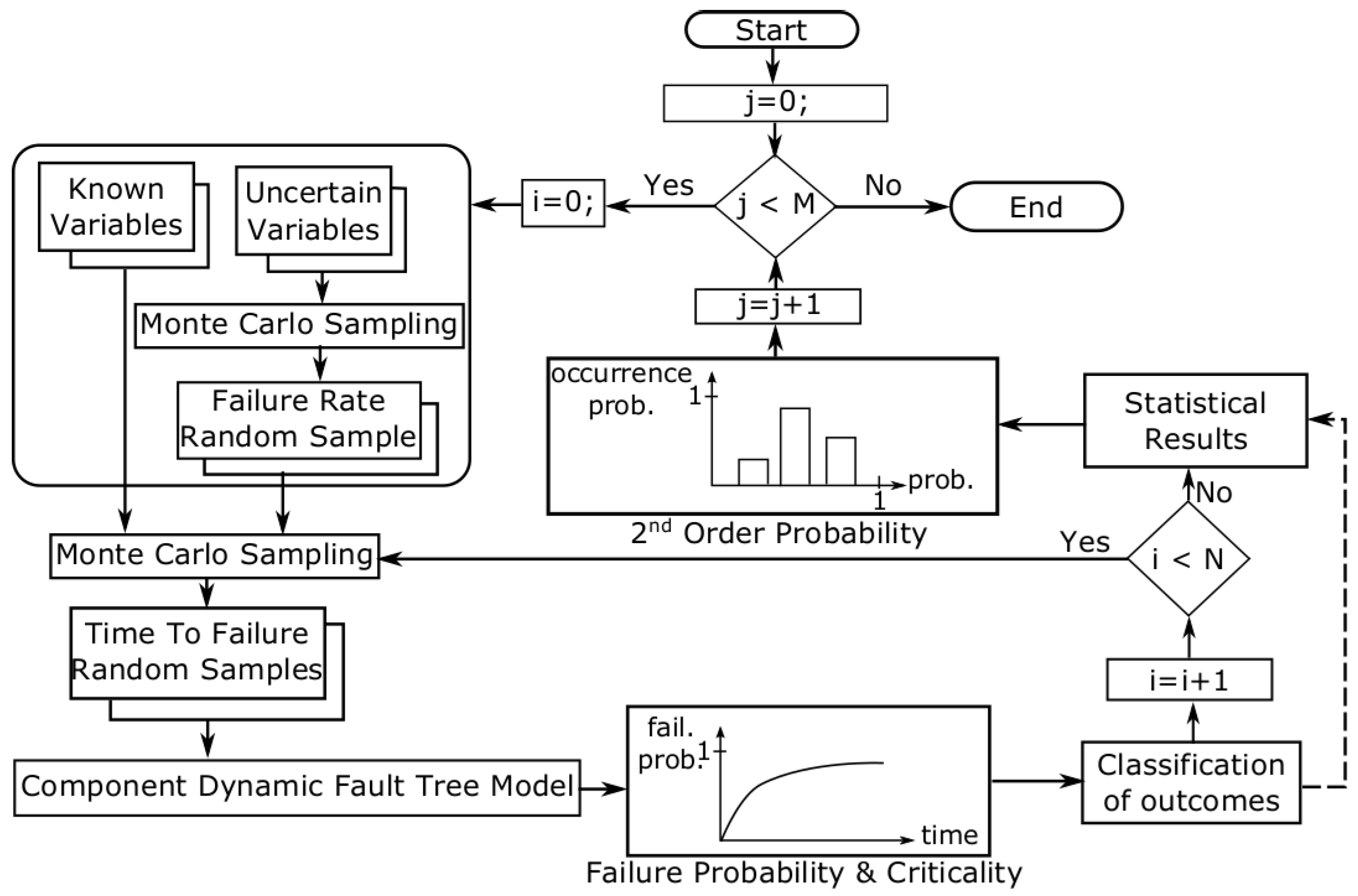
Figure 7 shows the overall evaluation process.
The following activities are involved in the analysis process:
Monte Carlo sampling of the uncertain variables: from the failure rates of the uncertain variables, a single failure rate value is chosen randomly within the specified failure rate interval according to the uniform distribution. A randomly sampled failure rate is the outcome of this activity.
Monte Carlo sampling of the time to failure of uncertain variables and known variables from their cumulative distribution function. A set of randomly sampled time to failure instants are the outcome of this process.
With the updated values, the CDFT model is solved extracting counters of top-event failure occurrences and critical event failure occurrences.
After N Monte Carlo trials, the CDFT model’s statistical results are gathered in a histogram which illustrates and classifies the frequency of occurrence of the top event.
After M Monte Carlo trials, the process ends and the histogram is normalized.
To analyse CDFTs, the MatCarloRe tool has been extended [
35]. The main drawback of this approach is the time needed for the computation of Monte Carlo simulations (
M×
N iterations in
Figure 7). While there are other techniques that reduce this time (e.g., dynamic stopping criterion [
36]), for the purposes of this study, we opted for using Matlab’s parallel toolbox in order to perform parallel tasks in several computers at a time.
4. D3H2 Application: Train Car Door Status Control
The Door Status Control is a safety-critical function that determines the safe operation of door open/close actions without endangering passengers’ safety [
18]. It has dependencies with other systems of the train and the doors open/closure operations are controlled by the driver depending on the status of the train, e.g., the doors must remain closed while the train is running.
Each door in the train has different sensors and control buttons for the passengers and the driver.
Figure 1 shows the Door Status Control configuration. There is one opening and one closing button for the driver connected to the driver’s PU (PU
Driver) and each door throughout the train has: one opening button for passengers, one door speed sensor, one door open detection sensor, one door closed detection sensor and one obstacle detection sensor. All these sensors, their controllers, and the door control algorithm are located in the PU
1.
In the train, there is a component called TCMS (Train Control and Monitoring System), which controls and monitors different critical systems of the train such as traction and doors. This component is homogeneously duplicated in two reliable PUs (PUTCMS) for safety purposes. The TCMS receives information about the speed of the train and it will not allow the driver to open the doors while the train is running. To this end, the TCMS sends an enable signal to the driver to inform the driver about the safe operation of door opening or closing (Enable Door Driver—EDD). Using the information of the Enable Door Driver signal, the driver sends an enable signal to the controller of each door (Enable Door Passenger—EDP) to act safely on opening/closing the doors, while taking into account if the train is moving and whether there is an obstacle in the door.
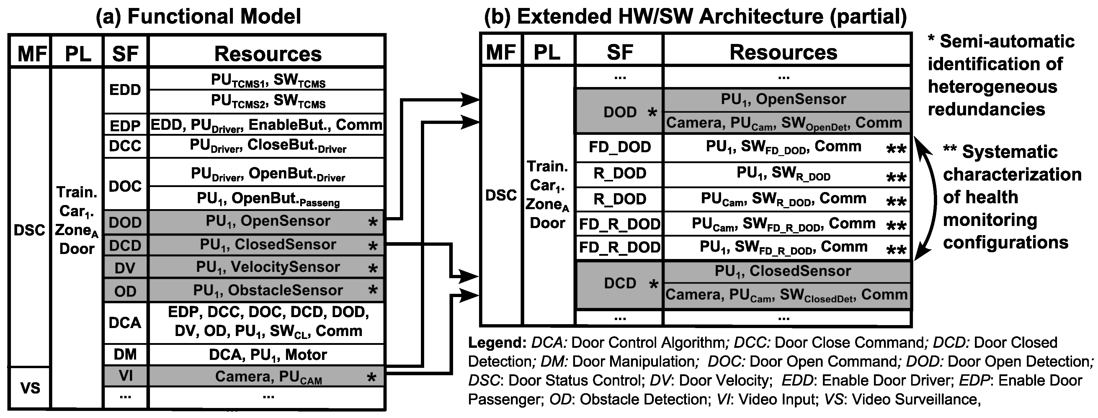
Figure 8a describes the functional model of the Door Status Control (DSC) main function, and the partial functional model of the Video Surveillance (VS) main function, which are both located at the same physical location: Train.Car
1.Zone
A.Door (
Figure 4).
The Door Status Control main function requires different input subfunctions to assure the safe operation of door opening/closing: enable subfunctions (Enable Door Driver—EDD, Enable Door Passenger—EDP), command subfunctions (Door Open Command—DOC and Door Close Command—DCC), and monitoring subfunctions (Door Open Detection—DOD, Door Closed Detection—DCD, Door Velocity—DV, Obstacle Detection—OD). Door open commands are generated by passengers and the driver, but the door close command is controlled only by the driver. These input subfunctions are directed toward the Door Control Algorithm (DCA) subfunction which determines when and how to close the doors through the Door Manipulation (DM) subfunction. Note that the final decision on opening/closing the door relies on the Enable Door Passenger (EDP) signal, which is determined by the driver.
The Video Surveillance function receives video images via the Video Input (VI) subfunction, processes them through the process image control subfunction and finally, if it is the case, it raises an alarm using the lamps and sirens connected to the PU
Cam. For clarity, only relevant information of the Video Surveillance main function is shown in
Figure 8a.
The extended HW/SW architecture of the Door Status Control main function includes all the nominal design decisions in the functional model (
i.e., EDD, EDP, DCC, DOC, DOD, DCD, DV, OD, DCA, and DM subfunction implementations (
Figure 8a)), design decisions with respect to possible redundancies for these subfunctions, and corresponding health management mechanisms to detect implementation failures and reconfigure between redundancies.
To identify possible redundancies, we apply the compatibility analysis focusing on
forced compatibilities because there are no matching subfunctions to consider heterogeneous redundancies arising from natural redundancies (
SubSection 3.2). After analysing all the I/O functions in the functional model located in compatible physical locations, we can observe that both Door Status Control and Video Surveillance are performed in the same (compatible) physical location. From this initial analysis, we can identify that there is a camera in each train car focusing towards the door. Based on engineering knowledge, we can come up with the heterogeneous redundancy implementations reusing the camera and its PU
Cam of the Video Surveillance main function.
Shaded cells in
Figure 8 identify heterogeneous redundancies. For clarity, we show heterogeneous redundancies only for DOD and DCD subfunctions, but note that the extended HW/SW architecture may include heterogeneous redundancies of OD and DV subfunctions as displayed in
Table 4.
To use these redundancies, the extended functional model must include fault detection and reconfiguration mechanisms.
Figure 8b shows the partial extended HW/SW architecture describing some heterogeneous redundancies (DOD, DCD) and design decisions for fault detection (FD_SF, FD_R_SF) and reconfiguration (R_SF) implementations and required resources. In
Figure 8b, we show a possible realization of the health monitoring mechanisms of the DOD subfunction using a single fault detection implementation (FD_DOD), duplicated reconfiguration implementations (R_DOD), and duplicated fault detection of the reconfiguration implementations (FD_R_DOD). The decision on the number and distribution of fault detection, reconfiguration, and fault detection of the reconfiguration is left to the designer. Note also that, for simplicity, we have omitted repeating subfunctions without redundancies in
Figure 8b (
i.e., EDD, EDP, DCC, DOC, DCA, DM—white cells in
Figure 8a), but these also are part of the complete extended HW/SW architecture.
The cost assessment is performed by adding up the cost of hardware and software resources. The cost of software components is quantified by considering their development cost assuming that it will be paid off in X years (let us assume X = 4 years for calculation purposes). We classify four types of software components: fault detection (SW_FD), reconfiguration (SW_R), fault detection of the reconfiguration (SW_FD_R) and Control/Detector (SW_Det). The development costs for each of these four software components is considered once for different subfunction implementations: once developed, they are adapted for the related subfunction implementations.
This assumption is adopted because the grouped subfunction implementations are closely related and costs therefore do not multiply (the cost of
N variants is not
N times the cost of a single software variant [
37]).
Fault detection implementations adapt to different subfunctions modifying subfunction-specific time/value thresholds. The development cost of
reconfiguration implementations does not differ for different subfunctions because reactivation logic holds the same.
Reconfiguration’s fault detection implementations differ only in the
keepalive timeout, and the development is independent of any subfunction. All the
control/detector software implementations have a similar logic.
Hardware cost: sensors, controllers and actuator costs are obtained from suppliers. The human cost related to mounting/testing is considered for sensors and actuators assuming ten minutes per sensor (actuator) at a rate of 60 €/hour.
Regarding failure rate values, resources with the same characteristics have been grouped. Pressure sensor covers open, closed and obstacle detection sensors. A processing unit carries all its different parameters; and communications (Comm.) include Multifunction Vehicle Bus (MVB) and Ethernet communication protocols and their gateway. Plausible values have been assumed for software components (
Table 5).
4.1. Redundancy Strategies
In order to analyse the effect of redundancy strategies, the reliability of the Door Status Control main function is analysed according to equations in
SubSection 3.4 for different Door Status Control configurations including homogeneous and heterogeneous redundancies.
Among the four input subfunctions with possible heterogeneous redundancies (DOD, DCD, OD, DV), alternative extended HW/SW architectures are analysed (
Table 6) adding one additional heterogeneous redundancy and/or homogeneous redundancy to each subfunction. The configuration of heterogeneous redundancies reuses the camera and requires a specific software component and communication resources, and the configuration of homogeneous redundancies includes a duplicated sensor for the specific subfunction (see
Figure 8b and
Table 4).
For each subfunction with redundancies, the fault detection and reconfiguration strategy shown in
Figure 8b for DOD subfunction is repeated. Denoting the set of subfunctions with redundancies as SF={DOD, DCD, OD, DV},
Table 7 displays the implementations of the health monitoring mechanisms with their corresponding resources used for the set of subfunctions with redundancies.
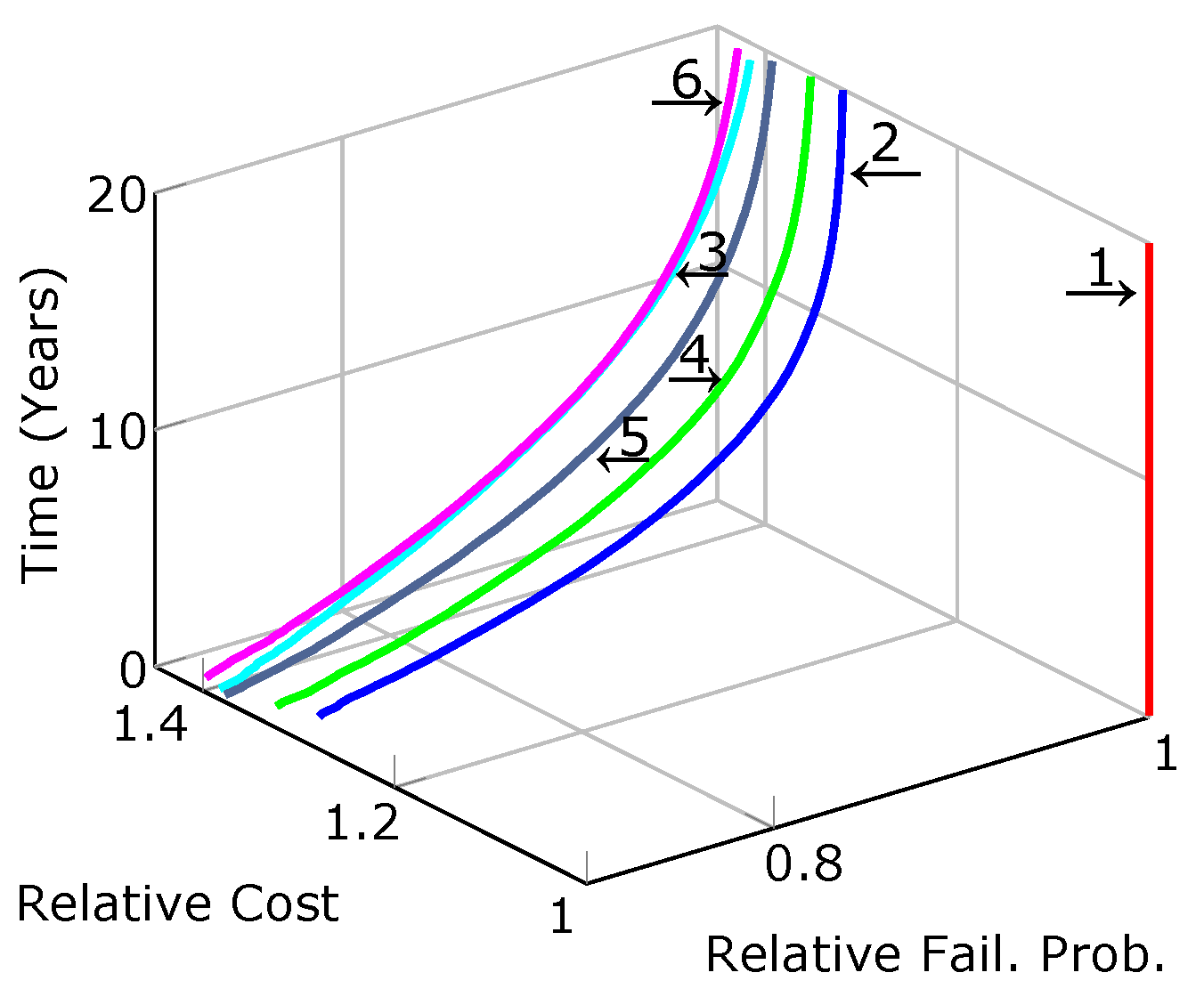
Figure 9 shows the DSC configurations’ relative cost and failure probability with respect to the DSC configuration without redundancies described in the functional model in
Figure 8a.
Figure 9 shows the relative improvement on the design of the Door Status Control main function for the studied train car, when including different types of redundancies. Results confirm that heterogeneous redundancies are more economical than homogeneous redundancies (see also
Table 8). However, the need of additional mechanisms (software) to make implementations compatible leads to having slightly worse reliability than homogeneous redundancies.
To analyse further differences between redundancy strategies, Failure Criticality Index (FCI) evaluations have been performed calculating for each component
i [
41]: the ratio between the number of system failures caused by the component
i to the total number of system failures. To deal with the lack of exact knowledge of the failure data of the software components, we have integrated the uncertainty analysis of SW_Det component’s failure data with the FCI assessment (see
SubSection 3.4.4).
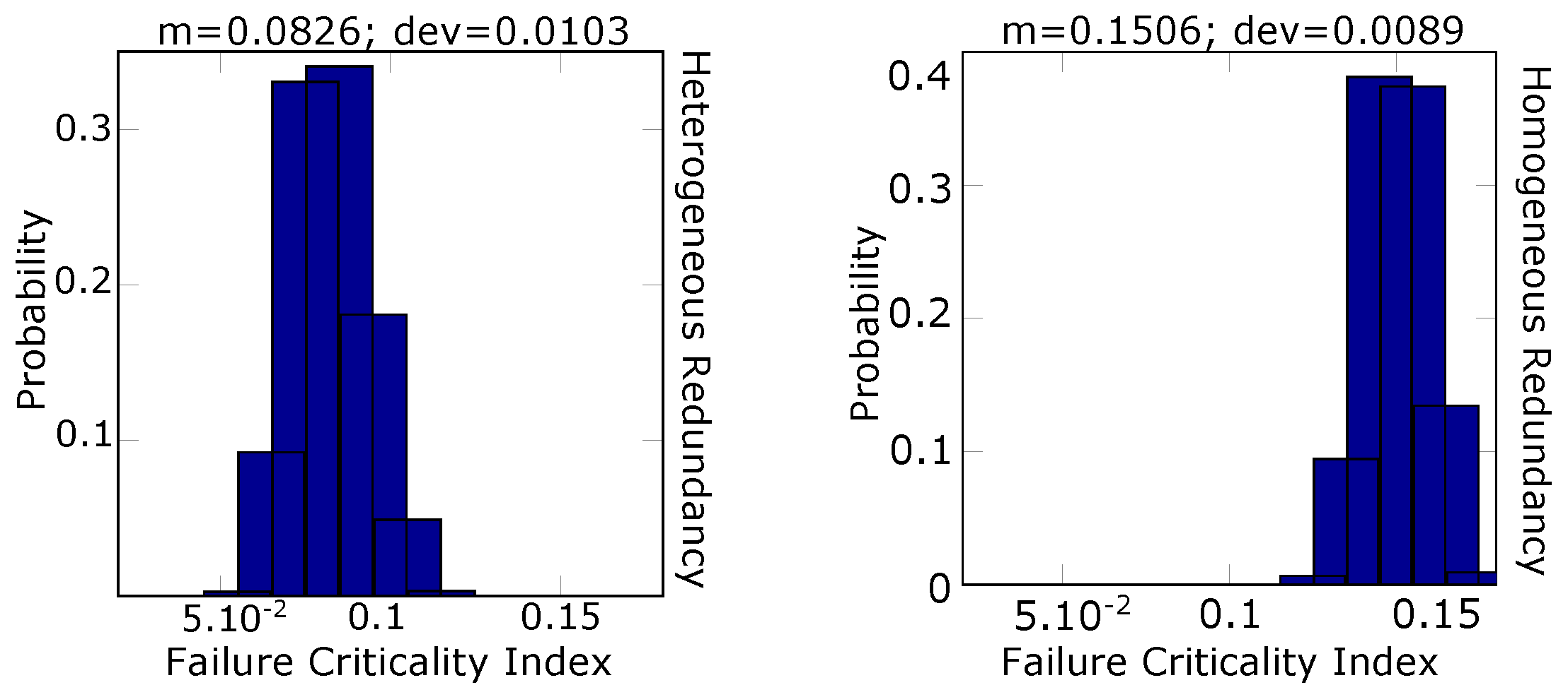
Figure 10 shows the distribution of the FCI values of Door Open Detection subfunction’s redundancy components with
= [0.001–0.1].
In a homogeneous redundancy configuration, duplicated sensors are connected to the same processing unit, while in the heterogeneous configuration, the camera is connected to one unit and the original sensor is in another unit (see
Table 4). From
Figure 10, we can see that the reuse of the unit adds bottlenecks to the system design resulting in a worse FCI than distributing tasks among different units.
4.2. Reconfiguration Strategies
To analyse the influence of the number and distribution of reconfiguration implementations on system dependability, this nomenclature is adopted in
Table 9: SF
i refers to the
ith implementation of the subfunction; 1R, 2R and 3R identify the number of reconfiguration implementations; and
C and
D letters designate centralised and distributed configurations, respectively.
Based on configuration #2 (
Table 6), alternative reconfiguration strategies have been tested with different failure rate values of health monitoring software components (
λSW_HM): SW_FD, SW_R and SW_FD_R. The failure rates of these components have been modified altogether to highlight the influence of reconfiguration implementations on system failure probability.
Table 9 displays failure probability values of the DSC main function for alternative reconfiguration strategies with different failure rate values of health monitoring software components. For instance, the configuration 2R C is the same as the architecture described in
Figure 8b (including heterogeneous redundancies for OD and DV in
Table 4 and repeating the health monitoring configuration of the DOD subfunction for DCD, OD, and DV according to
Table 7) and the configuration 2 of
Figure 9 (PU
Cam = PU
2).
From
Table 9, two main patterns are identified: the greater the
λSW_HM and number of reconfiguration redundancies, the better the failure probability of distributed reconfigurations. The failure probability of centralised reconfigurations confirms that the introduction of additional components increase system failure sources. However, with the increase of the failure rate values and reconfiguration’s redundancies, the system’s common cause failures gain importance, and distributed implementations perform better than configurations with system bottlenecks. Interestingly, there is a “threshold” failure rate, beyond which the distribution of reconfiguration strategies has no impact on the failure probability of the system. The “threshold” failure rate decreases as the number of reconfiguration’s redundancy implementations increases (see grey cells in
Table 9). This should be studied further, but it seems reasonable that the higher the failure probability of the reconfiguration implementations, the impact of the reconfiguration strategies becomes less important.
4.3. Health Management Mechanisms and Communication Influences
Taking configuration #2 of
Table 6 as the
reference configuration (with redundancies in
Table 4 and health monitoring mechanisms in
Table 7),
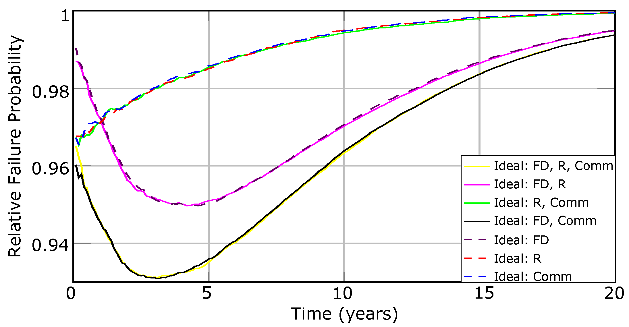
Figure 11 depicts the results of different architectures to test the influence of ideal fault detection, reconfiguration, and communication implementations. The outcome failure probability of different configurations has been normalized with respect to the
reference configuration, in which the behaviour of the fault detection, reconfiguration and communication implementations have been considered with their respective failure characterization.
As
Figure 11 shows, there is a 7% maximum difference between the ideal and the reference configurations in which the fault detection, reconfiguration and communication implementations are assumed perfectly reliable (
cf. yellow line). The influence of the failure behaviour of the fault detection is also noticeable (dashed purple line) caused by the lack of redundancy implementations.
To further evaluate the influence of the fault detection and reconfiguration subfunction failures on system failure occurrence, FCI evaluations have been performed for configurations #2 and #3 in
Table 6 (with redundancies in
Table 4 and health monitoring mechanisms in
Table 7). Two arrangements have been tested for configuration #3: connect explicit homogeneous sensors to the same PU or connect explicit homogeneous sensors to different PU
s.
Table 10 displays FCI values of fault detection (
) and reconfiguration subfunctions (
) for different Redundancy Strategies (RS).
In agreement with
Figure 11,
Table 10 displays that the FCI values of fault detection subfunction failures have higher criticality than reconfiguration subfunction failures.
Table 10 also confirms that concentrating redundancies in the same unit increases the influence on the system failure occurrence of fault detection and reconfiguration subfunctions (
Figure 10).
To check the consistency of the data depicted in
Figure 11,
Table 11 displays the FCI values of alternative subfunction failures under different assumptions: Door Control Algorithm (
) and Door Open Detection (
) as an example of input subfunction’s failure influence. The failure influences of the reconfiguration sequence of the Door Open Detection (
) and fault detection sequence of the Door Open Detection (
) on the system failure occurrence have also been analysed (see Equations (
7) and (
8), respectively).
Figure 11 and
Table 11 are in agreement: the ideal architecture is the least critical architecture and the real reference model is the most critical. Furthermore, we see that the fault detection has greater influence than reconfiguration and communication. For example, let us focus on the column
: while assuming ideal reconfiguration and communication implementations creates a difference of 0.14% and 0.129% from the FCI of the
reference configuration respectively, assuming ideal fault detection implementation makes a 0.584% difference with respect to the
reference configuration.
Focusing on the column , we can see that the configuration which assumes ideal fault detection (and combinations thereof with ideal reconfiguration and/or ideal communication) implementation has the biggest difference with respect to the reference configuration. Note that the Door Open Detection subfunction is one of the contributors to the system failure occurrence, but not the only one; the remainder of input subfunctions, the door control algorithm subfunction and the door manipulation implementation’s resources also has an influence.
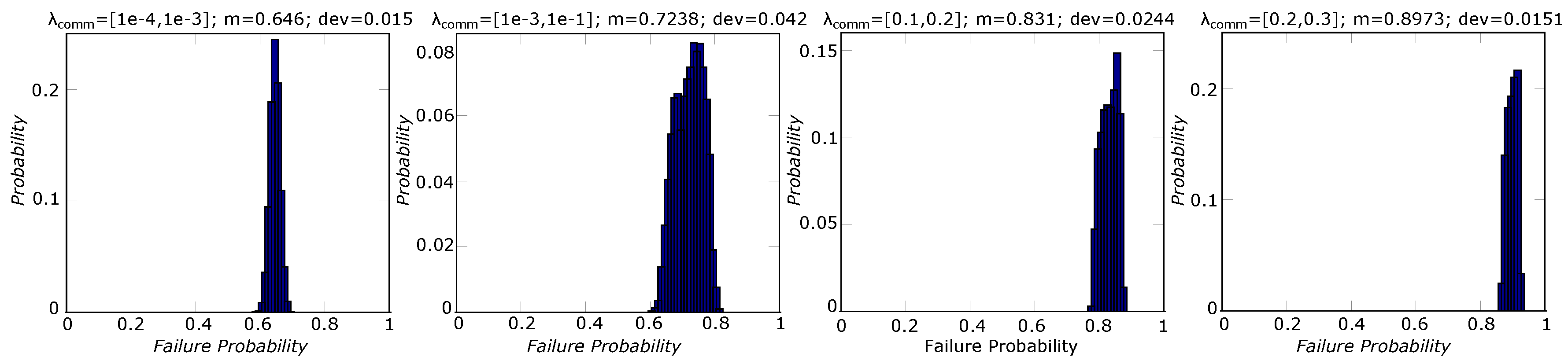
Finally, to analyse the influence of the communication on system failure probability, we have implemented uncertainty analyses assigning different interval values to the communication’s failure rate (
). Accordingly, we have analysed its influence on the distribution of the system failure frequency at the time instant T = 5 years for the configuration #2 in
Table 6 with health monitoring mechanisms shown in
Table 7 (
Figure 12).
As
Figure 12 confirms, an increase in
results in deterioration of the system’s failure probability. The mean and deviation of the system’s failure probability distribution depend on the failure rate interval.
5. Conclusions
In this paper, we have demonstrated how D3H2—a recently proposed analysis methodology—assists in the systematic assessment of the influence on dependability and cost of the location, type, and level of redundancy and reconfiguration implementations. The dependability evaluation model used by D3H2 is capable of analysing a range of sophisticated general failure patterns that may cause system failure. These include the potential failure of fault detection and communication implementations. The analysis capabilities include dealing with dynamic scenarios and uncertainty in failure characteristics data which is typical in the case of software components.
The influence of heterogeneous redundancies on system dependability and cost largely depends on the analysed system. In the case study presented in this paper, influencing factors included additional homogeneous sensors, software components for heterogeneous redundancies, and the impact of communication failure rates on heterogeneous redundancies. Heterogeneous redundancies show slightly lower reliability than homogeneous redundancies due to the added resources needed to make implementations compatible. However, as a result of the presence of common cause failures in homogeneous configurations, their failure criticality is higher than heterogeneous redundancies. Regarding the incurred cost, sensors need to be paid for for each introduced additional redundancy while software components are developed once and can be replicated across different implementations. Replication of software must be done with care to avoid the use of identical software in cases where common cause failure is relevant. Hence, the greater the number of redundancies, the cheaper becomes a solution that uses heterogeneous redundancies.
The influence of reconfiguration distribution strategies have been analysed emphasizing the following conclusions: as the number of reconfiguration redundancies or failure rates of reconfiguration software components increase, distributed reconfiguration strategies perform better than centralised reconfiguration strategies and the higher the unreliability of the reconfiguration implementations, the less important the impact of the distribution strategies becomes. The failure contribution of health management mechanisms and communication implementations needs to be evaluated for each architecture. As confirmed by the results, the influence of these implementations is defined by their criticality with respect to the system design.
Overall, D3H2 enabled a sophisticated and detailed assessment of the example system and enabled us to develop insights into the possible use of redundancy for achieving an improved trade-off between reliability and cost in this case. The study has also shown limitations of D3H2 and points towards further work:
- (a)
The formal identification and categorisation of heterogeneous redundancies for complex systems is a challenging task. The lack of deterministic relations between some of the variables hampers the formalisation process. Possible solutions to address these issues can include formalisation of engineering design knowledge through meta-modelling techniques (e.g., [
42]) or formal analysis of highly networked scenarios through equation-based modelling formalisms (e.g., [
43]).
- (b)
We have not included downtime costs arising from repair activities, which leads to high financial penalties due to the immobilization of trains on stations or tracks. For our future goals, we plan to perform the following activities: (1) introduce repair concepts to evaluate availability and downtime costs; (2) automate the architecture optimisation extracting the combination of homogeneous and heterogeneous redundancies, which maximizes dependability and minimizes cost, e.g., by extending work on metaheuristics in [
14]; and (3) weigh the degradation of the functionality considering other factors than component failure rates.
- (c)
While for non-repairable systems only the order of failure is important, for repairable systems, both the order of failure and repair must be respected. In D3H2, the reconfiguration process is governed by the reconfiguration priority of implementations. This means that the reconfiguration process is not necessarily a sequential process, but it can follow a random process. Therefore, the predefined sequential logic of repairable Dynamic Fault Tree gates [
24] is invalid for repairable systems. More powerful and flexible stochastic formalisms are needed to address these properties (e.g., [
44]).
- (d)
Finally, with the dependability evaluation model presented in this paper, there is potential for automation and optimization via use of metaheuristics. Fitness functions can include dependability and cost while parameters to be altered may include the location, type, and level of redundancies and health monitoring mechanisms. Metaheuristics can focus on choosing solutions for these variables that could optimize the trade-off between dependability and cost.


 ,
, 


