Preliminary Results of Clover and Grass Coverage and Total Dry Matter Estimation in Clover-Grass Crops Using Image Analysis

Abstract

The clover-grass ratio is an important factor in composing feed ratios for livestock. Cameras in the field allow the user to estimate the clover-grass ratio using image analysis; however, current methods assume the total dry matter is known. This paper presents the preliminary results of an image analysis method for non-destructively estimating the total dry matter of clover-grass. The presented method includes three steps: (1) classification of image illumination using a histogram of the difference in excess green and excess red; (2) segmentation of clover and grass using edge detection and morphology; and (3) estimation of total dry matter using grass coverage derived from the segmentation and climate parameters. The method was developed and evaluated on images captured in a clover-grass plot experiment during the spring growing season. The preliminary results are promising and show a high correlation between the image-based total dry matter estimate and the harvested dry matter $(R^2=0.93)$ with an RMSE of 210 kg ha${}^{-1}$.

1. Introduction

The clover content has a great influence on growth and herbage quality in a clover-grass crop and on the effect of different cultivation management strategies. The rate of nitrogen (N) fertilization is normally the same for all clover-grass fields on the farm. However, the N-response is shown to decrease with increasing clover content, sward age and N-strategy through the growing season [1]. The N-utilization could therefore be improved for the individual field and for the whole farm, if the N-rate and -strategy are adjusted to the spatial distribution of clover content and sward age.

Knowledge about the clover content is also advantageous when composing feed ratios for livestock. A high clover content can increase the dairy cow forage intake and increase milk production [2]. However, clover must be seen as part of the optimum forage plan and has to be balanced towards other forage sources. Information of crop biomass and clover-grass ratio is therefore important when planning the management in the field and evaluating the forage plan. A common approach to determining the clover content in a field is through a destructive analysis. However, this method is very cumbersome and costly and therefore not used in practice. Hence, a simple non-destructive tool to quantify the clover and grass content would be an important tool in a Farm Management Information Systems (FMIS) and in the farmer’s decisions to optimize forage plans in order to increase milk production and thereby net revenue.

A simple non-destructive solution is to use a camera to capture images of the field and, based on the clover and grass coverage in the images, estimate their respective dry matter (DM) contribution. The images could be captured by a smartphone, a camera mounted on a tractor or an implement, or perhaps a drone mapping the entire field. Common and essential for these three cases is that they use a camera and require image analysis to extract the clover and grass coverage from the images.

1.1. Related Work

In the wider context of dry matter estimation, several non-destructive approaches have been explored in the literature. Closely related to legume-grass mixtures, these methods include growth models [3], spectrometry [4], remote sensing [5] and computer image analysis [6,7,8].

Crop growth models seek to predict the crop yield by modeling the growth of the crop through its internal processes, the surrounding temperature and the availability of nutrients, water and light. These growth models may consider a single species such as perennial ryegrass in the LINGRA (LINTUL-GRASS: Light Interception and Utilization simulator - Grass) model [9], timothy [10] and meadow bromegrass [11] in CATIMO (Canadian Timothy Model) or the interaction between species such as ryegrass and white clover in the GrazeGro model [3]. The growth models are designed for regional yield forecasting and are therefore not suitable for describing the local spatial variability.

Remote sensing using satellite or aerial systems has been widely studied for vegetation classification [12] and mapping [13], as well as yield estimation [14]. Remote sensing systems typically rely on multi- or hyper-spectral imaging systems, but may also employ radar [15] or LiDAR [16]. However, satellite-based remote sensing is sensitive to the cloud cover in a region, which makes it hard to reliably get repeated measurements in a given area [17]. Commonly, the spatial resolution of remote sensing systems is very low compared to ground-based systems, but with the recent emergence of Unmanned Aerial Vehicles (UAVs), the gap in spatial resolution between remote sensing and ground-based systems is beginning to close.

Biewer et al. [4] explored using four different vegetation indices derived from a field spectrometer to predict the total biomass and species proportions in legume-grass mixtures. Despite a strong correlation between the vegetation indices and the total biomass, the indices were unreliable for large biomasses, where the indices start to saturate as the canopy closes. Furthermore, they found variations in biomass to have a much larger effect on the vegetation indices than the legume-grass ratio, thereby making it difficult to determine the species proportions without a fixed biomass. To mitigate this, they suggested in future work combining field spectrometry with image analysis.

Using computer vision to detect and recognize plants in fields has been widely studied [18,19,20]. However, common for most of these cases is that they have challenges with overlapping leaves and shadowing, and they primarily regard weed as isolated from other plants [21]. Gebhardt et al. [22] developed an algorithm for the detection of broadleaved dock (Rumex obtusifolius L.) in grassland, which was later expanded upon by Gebhardt and Kühbauch [23]. They achieved a 90–95% detection rate by using a set of shape, color and texture features to distinguish this weed species from other species. Bonesmo et al. [6] have developed a method for estimating the coverage of white clover (Trifolium repens L.) and smooth stalked meadow grass (Poa pratensis L.) in digital images using image processing. They considered images that are covered with 0–22% clover and are able to estimate the coverage with a root mean square error of 2.5%-points. However, they did not relate the coverage to dry matter content. Himstedt et al. [7] have investigated the relationship between the coverage and the dry matter distribution of binary legume-grass mixtures for white clover (Trifolium repens L.), red clover (Trifolium pratense L.) and alfalfa (Medicago sativa L.). Based on a calibration model developed in a pot experiment, they were able in a field experiment to estimate the legume dry matter contribution by manually labeled images. Their dataset considered biomasses from 216–2819 kg ha${}^{-1}$ and coverage from 0–100%. The dry matter contribution RMSEs were 58.9 g kg${}^{-1}$ and 43.1 g kg${}^{-1}$ for red and white clover, respectively. However, they relied on knowing the total dry matter production for estimating the dry matter contributions. Recently, McRoberts et al. [8] have proposed a rotational invariant method for estimating the grass fraction in digital images of grass and alfalfa. Their proposed method used histograms of local binary patterns for estimating grass coverage and showed a strong correlation between the estimated grass coverage and actual grass fraction.

Recent developments within deep convolutional neural networks have shown impressive results on computer vision tasks such as image classification [24,25] and pixel-wise classification [26,27]. Recently, these deep neural networks have also been adopted in the agricultural domain [28,29]. Deep neural networks, however, require large amounts of data containing thousands of examples to be trained, which makes them hard to employ in tasks, where the ground truth data are very expensive to collect.

Although the clover contribution can be estimated accurately using the method proposed by Himstedt et al. [7], the total dry matter is required to estimate the individual species contributions. In this paper, we propose a system to automatically estimate the total dry matter of clover (red and white) and grass (perennial ryegrass (Lolium perenne L.) and festulolium) in the sward from digital images using image analysis and present the preliminary results of this system. The method for segmenting the clover and grass used in this paper is based on the method proposed by Bonesmo et al. [6]; however, the method is expanded upon, and several improvements are proposed and implemented.

Our contribution is three-fold: (1) we present a method for distinguishing between RGB images captured under different illuminations; (2) we expand on the image analysis method proposed by Bonesmo et al. [6] for estimating clover and grass coverages; (3) we present a model for estimating the total and individual dry matter content of clover and grass using only the coverage and climate parameters.

2. Materials and Methods

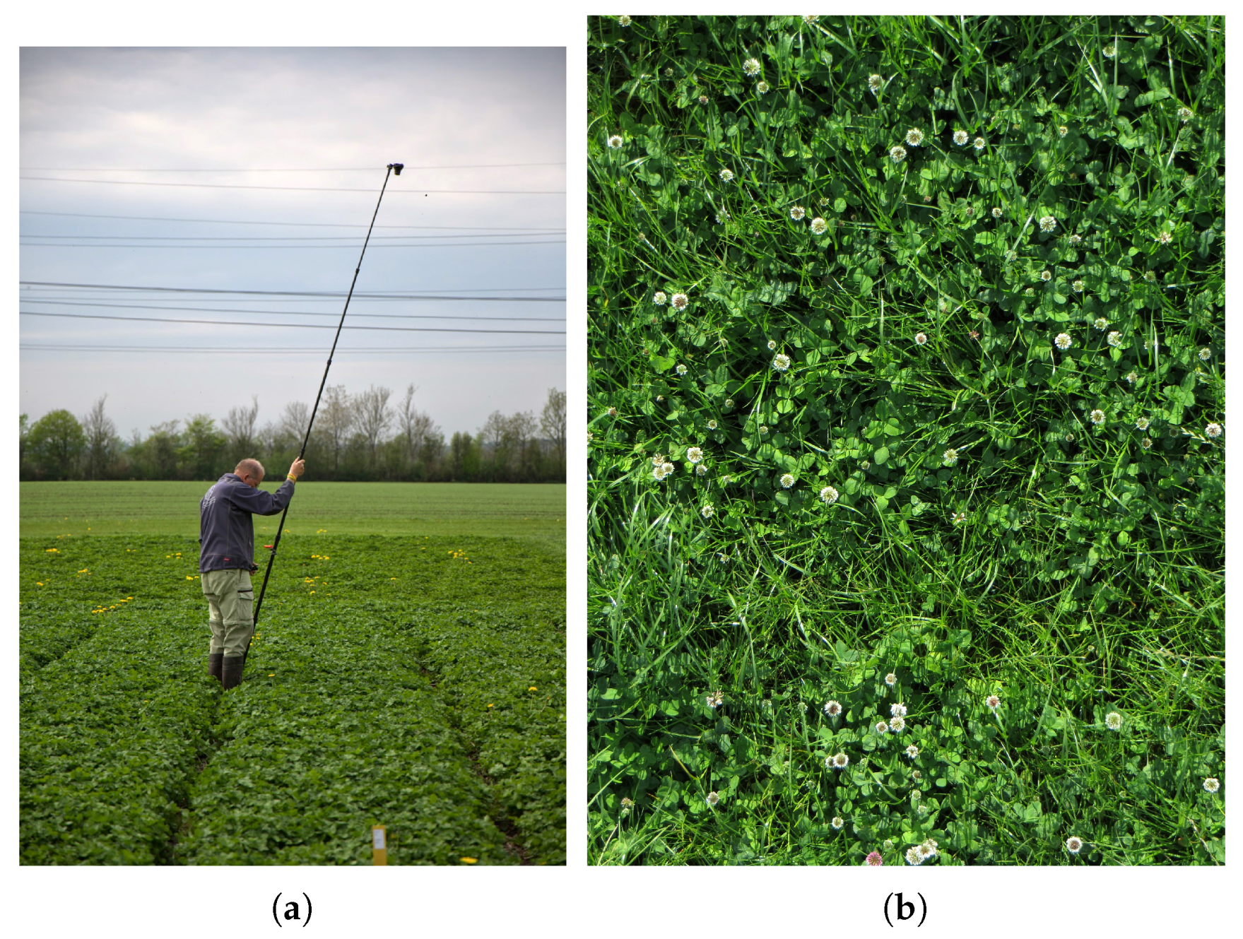
2.1. Testbed and Data Acquisition

The present study was part of a larger experiment, where the purpose was to evaluate different cutting strategies in two clover-grass mixtures and one pure red clover crop. The plot experiment was carried out in 2013 at Research Center Foulum, Denmark (56.495749° N, 9.566237° E). All plots were established in spring 2012 by undersowing clover and grass in spring barley. In the 2013 growing season, image capturing in the present study and plant sampling from the larger experiment coincided on three occasions during the summer and fall (

Table 1. Photograph and cutting dates, number of samples, cut number and solar azimuth and altitude on the photo date for each occasion.

	1st Occasion	2nd Occasion	3rd Occasion
Photo Date	25 June	10 September	11 October
Cutting Date	25 June	11 September	14 October
Samples	10	5	30
Cut Number	2	4	4, 5
Solar Azimuth	29–33°	36–37°	24–25°
Solar Altitude	90–97°	199–203°	155–164°

). The number of samples at each occasion varied due to the experimental plan in the larger experiment. Data used in the present study came from a selected subset of plots with clover-grass mixtures from the larger experiment. In total, 45 images coincided with plant samples from 14 plots (2 clover-grass mixtures with 7 plots each) across the three occasions.

Each plot had a size of 1.5 m × 10 m. Two different seed mixtures were used, which consisted of (1) 87% perennial ryegrass and 13% white clover (“Mixture 35”) and (2) 37% perennial ryegrass, 45% festulolium, 11% red clover and 7% white clover (“Mixture 45”). All plots were fertilized with 150 kg K ha${}^{-1}$ at initiation of spring growth and with 160 kg N ha${}^{-1}$; 100 kg N ha${}^{-1}$ at initiation of spring growth and 60 kg N ha${}^{-1}$ after first cut.

After cutting, a subsample of the biomass was dried and separated into white clover, red clover, grass and weed. Each group was dried to constant weight, and the dry matter content in each group was recorded. The total amount of herbage dry matter ranged from 195–3084 kg ha${}^{-1}$. The content of white clover, red clover, grass and weed ranged from 4–46%, 13–52%, 26–90% and 0–3% DM, respectively. The combined clover (white + red clover) content ranges from 10–72% DM.

Up to three days prior to cutting the plots, the plots were photographed with a Canon Powershot 260 HS digital camera mounted on a pole (Figure 1a). The capture time during the day varied from 9 a.m.–2 p.m. The images were captured and stored in JPEG-format with a resolution of 3000 × 4000 pixels. The photos were taken from directly above the plot and covered approximately 0.80 m × 1.00 m (Figure 1b) giving approximately 4 pixels mm${}^{-2}$. Within each plot, two photos at two different locations were taken. The capturing was performed on three different dates from June–October (Table 1). During capturing, two different illuminations were experienced, direct sunlight and indirect sunlight, causing different levels of shadowing. The average hourly solar irradiance was 98 W m${}^{-2}$ in indirect sunlight and 382 W m${}^{-2}$ in direct sunlight. The solar azimuth and altitude varied between dates and time of date and are summarized in Table 1. For each of the 45 images in the dataset, the dry matter content of the species in the sward is known, but the true coverage of clover and grass is unknown. From the image dataset, 28 patches (150 × 250 pixels) were randomly extracted, and soil, grass, clover, clover seed heads, weed and unknown were manually annotated pixel-wise in each patch. The manual annotation was performed by manually tracing the contour of each class. When the contour was closed, all pixels within it were labeled as the same class, which was specified by the user. Examples can be seen in Figure 2. The 28 patches were divided into a training and test set with a 60/40% split.

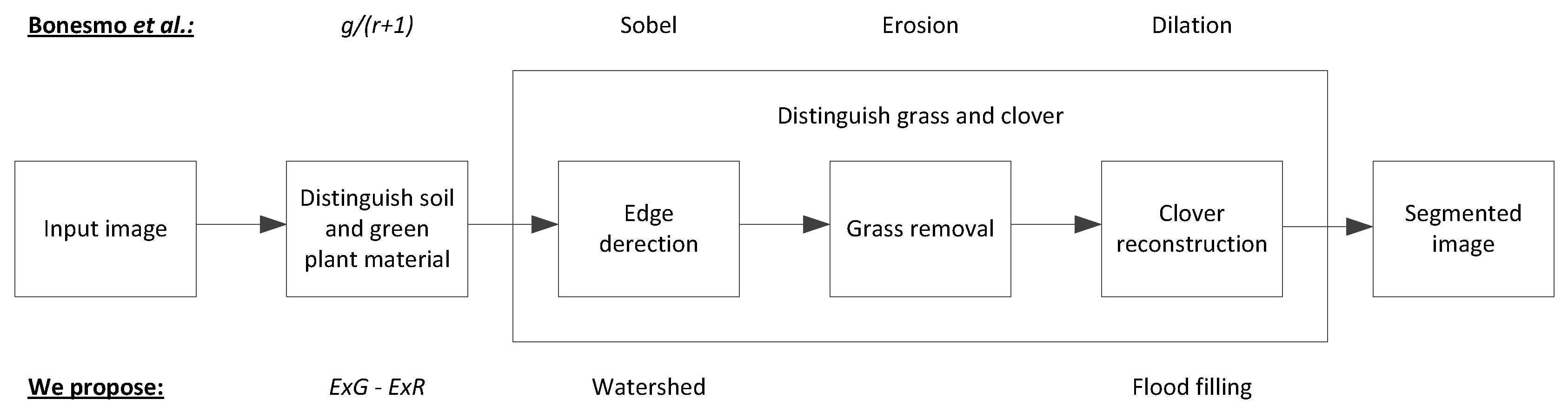
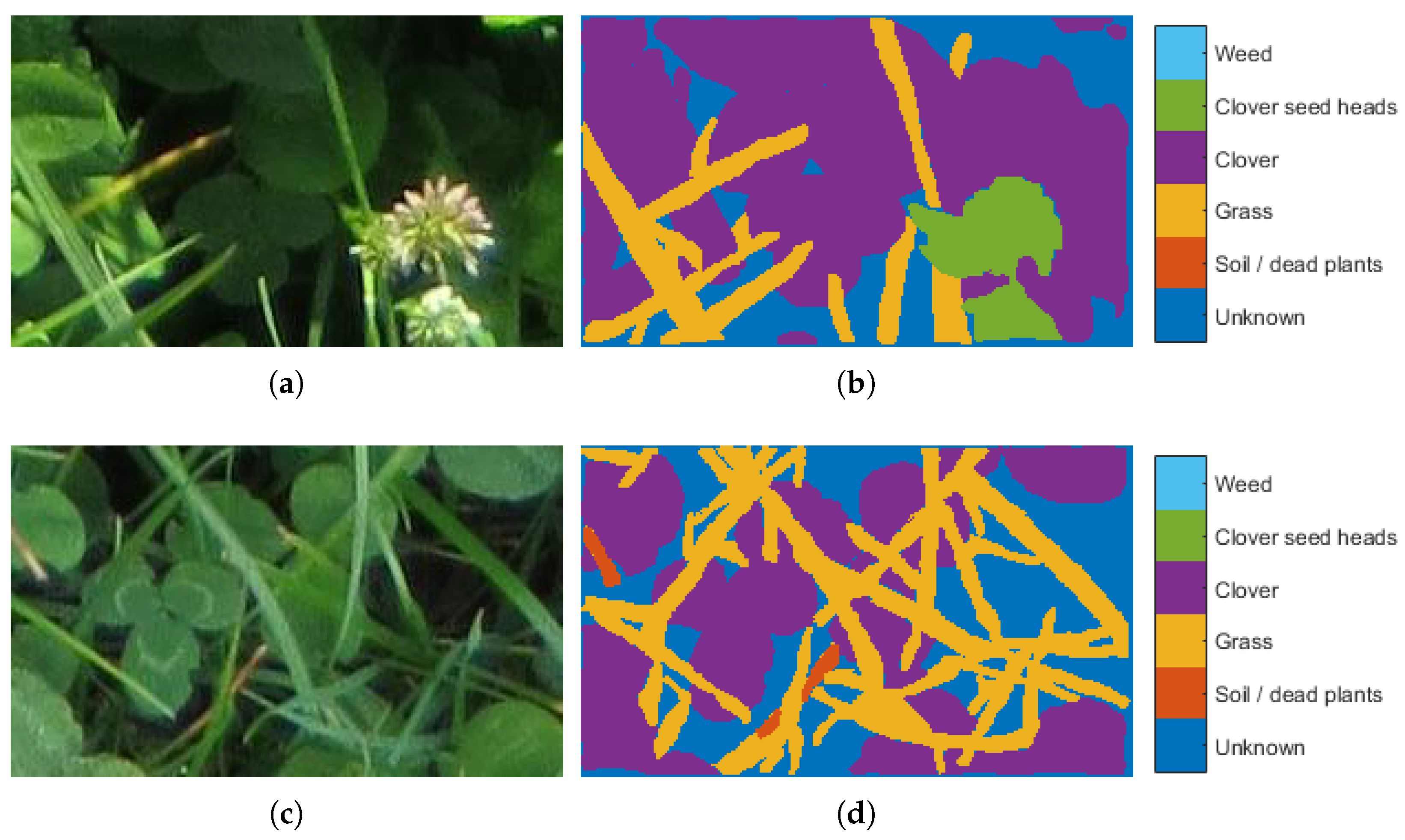
2.2. Clover-Grass Segmentation

To segment the images into soil, clover and grass, we explored the method proposed by Bonesmo et al. [6]. As seen in Figure 3, the estimation of the coverage of clover and grass is done in two steps. In the first step, the background segment is found. It consists of regions with soil, dead plants and deep shadows, where deep shadows are formed by holes in the canopy. The foreground segment consists of a mixture of clover and grass. In the second step, the foreground is segmented into clover and grass regions. This is done by finding the edges between the leaves followed by a series of erosions on the inverted edge image to remove the grass. Finally, the clover is reconstructed from the remaining pixels after the erosion. The non-reconstructed foreground pixels are regarded as grass. We propose three alternatives for distinguishing soil and green plant material, edge detection and clover reconstruction, which are described in the following sections. Finally, we also propose a method for distinguishing between direct and indirect illuminations and classify an input image accordingly. Classifying the illumination allows for training of the segmentation algorithm on each type of illumination separately.

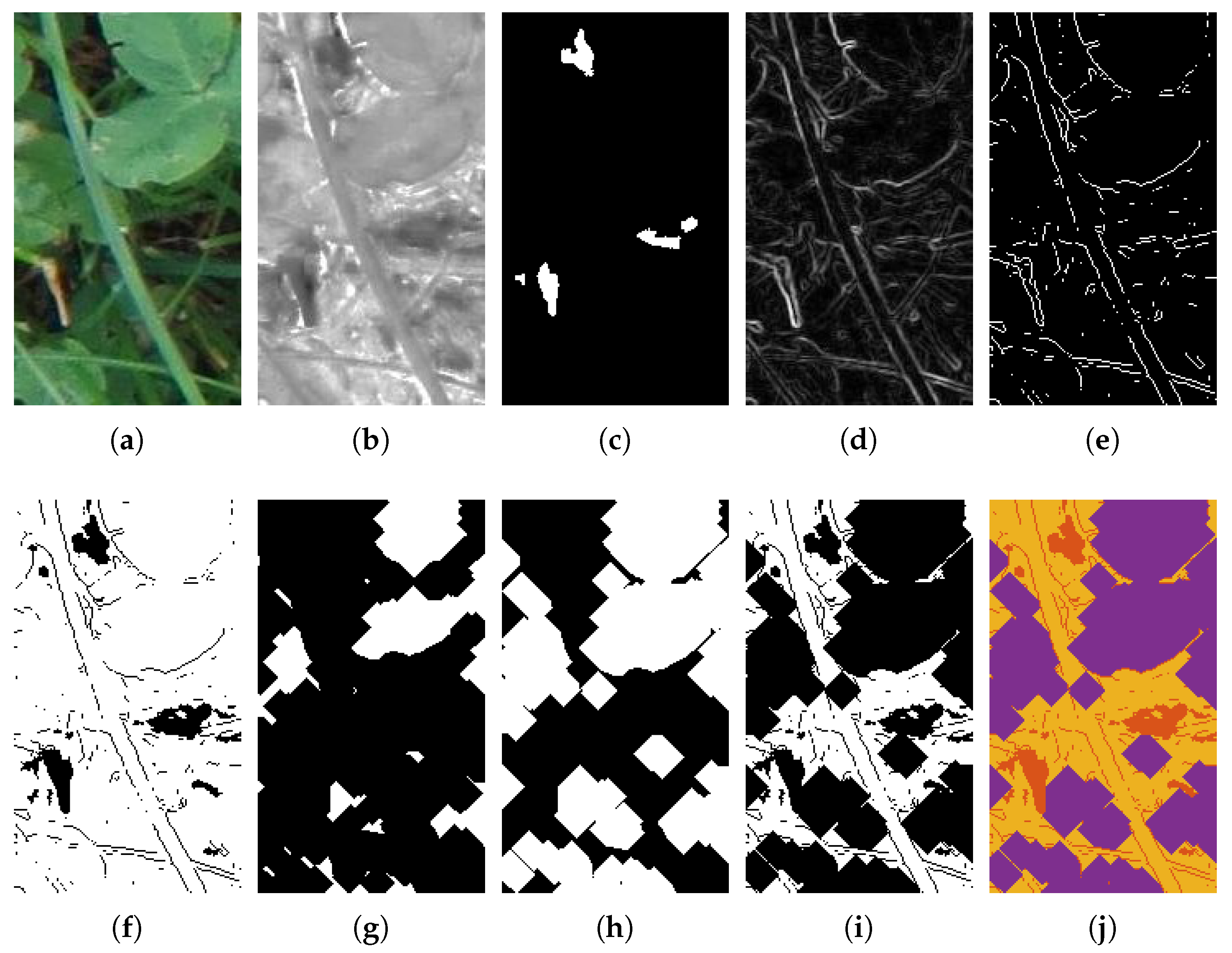
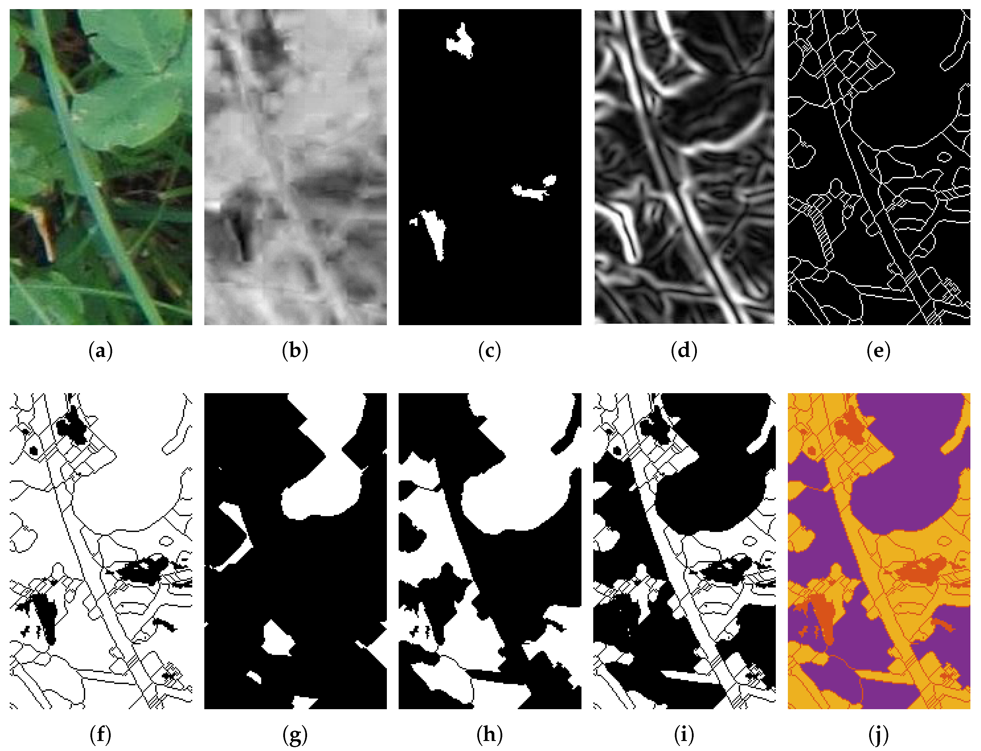
2.2.1. Distinguishing Soil and Green Plant Material

To distinguish between soil and green plant material, it is common practice to compare the red and green intensities pixel wise. More green indicates green plant material. More red indicates soil or dead plant material. Bonesmo et al. [6] uses the the ratio image, $I_{RG}(x,y)$, given by:

$$I_{RG}(x,y)=\frac{g(x,y)}{r(x,y)+1}$$

(1)

where $g(x,y)$ and $r(x,y)$ are the normalized green and red color components, respectively, at the image position $(x,y)$. The ratio image is thresholded to segment the background pixels (soil, dead plant material and shadows) from the foreground pixels (green plant material such as clover and grass) (Figure 4a–c). However, the effectiveness of the ratio image is not compared to any other similar method.

More recent work by Meyer and Neto [30] has shown that the difference ($ExGR$) in excess green ($ExG$) and excess red ($ExR$) is a good color vegetation index for distinguishing soil and dead plant material from green plant material. Therefore, the difference in excess green and excess red is evaluated as an alternative method in this context. Excess green, excess red and the difference are given by:

$$ExG(x,y)=2G(x,y)-R(x,y)-B(x,y)$$

(2)

$$ExR(x,y)=1.4R(x,y)-G(x,y)$$

(3)

$$ExGR(x,y)=3G(x,y)-2.4R(x,y)-B(x,y)$$

(4)

where R, G and B are the red, green and blue chromaticity of the image pixel, respectively. The green plant regions consist of pixels where $ExG$ exceeds $ExR$ by a certain amount. This amount is a tunable parameter, which must be learned during training (see Section 2.2.5). The complementary region consists of soil and dead plant material (Figure 5a–c). During development, preliminary results showed similar performance when using the normalized R, G and B values rather than chromaticity. Therefore, both color indices were evaluated. $ExG{R}_C$ and $ExG{R}_N$ are used to distinguish between using chromaticity and normalized color values, respectively.

2.2.2. Edge Detection

In the edge detection step, the edges between leaves are detected, and a binary edge image is created. The edges are used to segment the foreground into segments, where the larger segments correspond to clover leaves and the smaller and thinner ones correspond to grass leaves. To detect the edges, Bonesmo et al. [6] used the Sobel operator to generate a gradient image, which is subsequently thresholded to form the binary edge image (Figure 4d,e). Sobel is an excellent operator for determining the gradient of each pixel, but simply thresholding this gives a poor edge detection in our case. In the present case, it is not necessarily the edges with the strongest gradient that are of interest. Edges between leaves (both between clover and grass and between each species) tend to be lower than edges between the white marks on the clover leaves and the green part of the clover leaves. Secondly, the detected edges are not guaranteed to be closed.

To overcome these deficiencies, we used the watershed algorithm [31] on the gradient image to detect the edges. The watershed algorithm works by growing segments from the local minimums of the image. When two segments meet, an edge is formed between them. This process is continued until all pixels are either a segment or an edge. The watershed algorithm ensures that both weak edges can be detected and that all edges are closed.

Prior to estimating the gradient, the image was blurred using a zero mean Gaussian kernel with a standard deviation $\sigma$. Using a larger standard deviation will reduce the amount of false edges; however, it will also reduce the amount of true edges. Likewise, reducing the standard deviation will increase the number true edges, but also increase the amount of false edges. Before applying the watershed algorithm to the gradient image, the gradient image was thresholded to remove very small and noisy gradients (Figure 5d,e).

2.2.3. Clover Reconstruction

When the foreground has been segmented by the edge detection, each segment is morphologically eroded $N_E$ times by a $3\times 3$ circular structuring element [6]. After the sequence of erosions, any remaining segments are considered clover, and all segments, which were removed by the erosion, are considered grass (Figure 4f–i). To reconstruct the clover leaves, Bonesmo et al. [6] morphologically dilated the remaining segments using the same structuring element the same number of times as when they were eroded. However, dilating a remaining segment does not guarantee reconstruction of the original segment, as small features of the segments can be lost in the erosion process.

Instead, we used flood filling to reconstruct the remaining segments to preserve the shape of these segments. Flood filling iteratively grows an object from a seeding point using dilation. When the perimeter of the growing objects reaches a background pixel, it stops growing in that direction. We used a random pixel from each remaining segment after the erosion process as seed points for flood filling of the inverted edge image. In the inverted edge image, the edges are the background pixels, which stop objects from growing, when reconstructing the segments (Figure 5f–i). The downside of this method is that it requires a completely segmented image. Otherwise, it could recreate grass leaves, which prior to the erosion were connected to clover, but were removed during the erosion process.

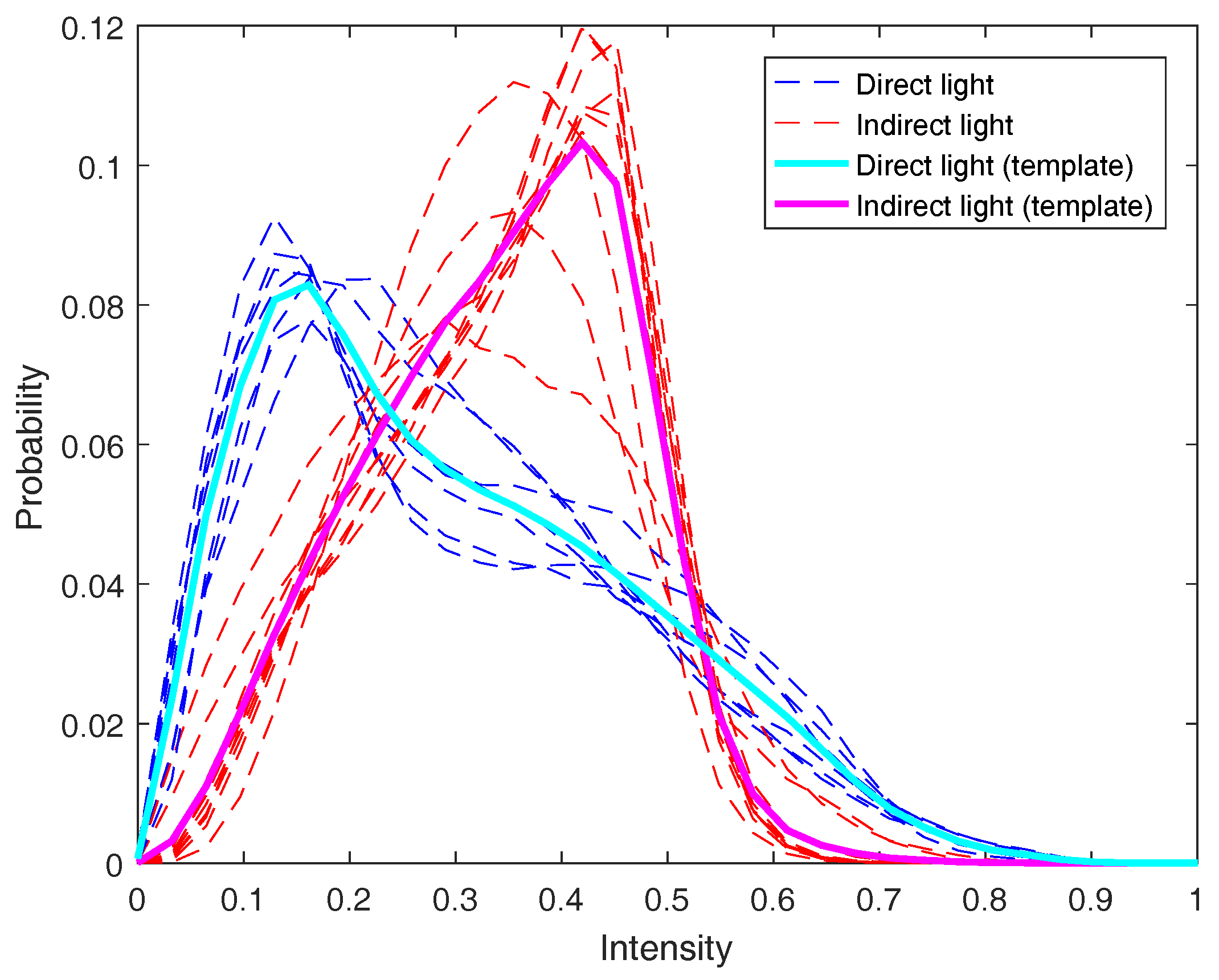
2.2.4. Illumination Classification

The illuminations vary due to different weather conditions. This causes different levels of shadowing in the recorded images to be dealt with during image analysis. The illumination was classified into two classes: direct light and indirect light. Direct light occurs when the Sun shines directly onto the field causing heavy shadowing from one leaf onto another leaf. Indirect light occurs in cloudy weather, where the clouds cause a more ambient and diffuse lighting, reducing the amount of shadows cast from one leaf onto another leaf (Figure 2a). The shadows cast from one leaf onto another greatly influence the edge detection and thus the size of the segments extracted. Therefore, a natural extension to the algorithm is to classify an input image based on its illumination and select a set of pretrained parameters based on the classified illumination.

The illumination for an image was classified by generating a histogram from the gray-scale version of the image where $ExG$ exceeded $ExR$. As seen in Figure 6, there is a clear difference in the histograms of the two classes. A mean histogram for each class was calculated, and they were used as the templates for the classes. Each new image was classified according to its correlation distance to each template histogram.

A coarse logarithmic grid search was used to determine the optimal image size and optimal number of bins in the image histogram. The mean histogram for both direct and indirect light was calculated for each combination of image scale and numbers of histogram bins based on the image training set. For each combination, the image validation set was classified based on the corresponding mean histograms from the image training set. The accuracy, which is the ratio of true classifications with respect to all classifications, was used as a metric to determine the best image scale and number of bins.

2.2.5. Training Clover-Grass Segmentation

The original algorithm of Bonesmo et al. [6], as well as the proposed improvements were implemented in MATLAB [32] and trained and evaluated on our dataset. To evaluate the performance of each proposed improvement, the original algorithm was trained without any improvements and with each of the improvements, as well as all combinations of the improvements. The training included finding the optimal set of parameters for both illuminations combined, as well as for each illumination individually.

The training was performed using a coarse grid search. The coarse grid search was followed by a fine grid search centered on the best performing set of parameters found in the coarse grid search.

The frequency-weighted Intersection over Union (fwIoU) was used as the training metric. The frequency-weighted intersection over union is given by:

$$\mathrm{fwIoU}=\frac{1}{{\sum }_K^{k=1}{t}_k}\sum _K^{i=1}\frac{n_{i,i}{t}_i}{t_i+{\sum }_K^{j=1}{n}_{j,i}-n_{i,i}}$$

(5)

where $n_{i,j}$ is the number of pixels from class i predicted to belong to class j, $t_i={\sum }_K^{j=1}{n}_{i,j}$ is the total number of pixels belonging to class i, ${\sum }_K^{j=1}{n}_{j,i}$ is the total number of pixels predicted to belong to class i and K is the total number of classes [26].

2.3. Dry Matter Estimation

The total dry matter was estimated using a linear model. The clover and grass coverages, temperature sum (>0 °C), accumulated sunshine hours and a factor variable showing which clover-grass mixture were in the individual plots were used as predictor variables. The model was found using stepwise linear regression (stepwiselm in MATLAB [32]), where terms and interactions were added or removed based on their significance ($p<0.05$ and $p>0.10$, respectively). The initial model to which terms were added and from which were removed was a strictly linear model:

$$DM={\beta }_0+{\beta }_1{C}_G+{\beta }_2{C}_C+{\beta }_{3}S+{\beta }_{4}T+{\beta }_{5}M$$

(6)

where $DM$ was the total dry matter, $C_C$ and $C_G$ are the clover and grass coverage, respectively, S is the accumulated sunshine hours since last harvest, T is the temperature sum since last harvest, M is a categorical variable describing the mixture (“Mixture 35” or “Mixture 45”) and ${\beta }_{0–5}$ are the weights of each term. The clover and grass coverages ranged from 0–1 and were calculated based on the results of the image segmentation.

3. Results

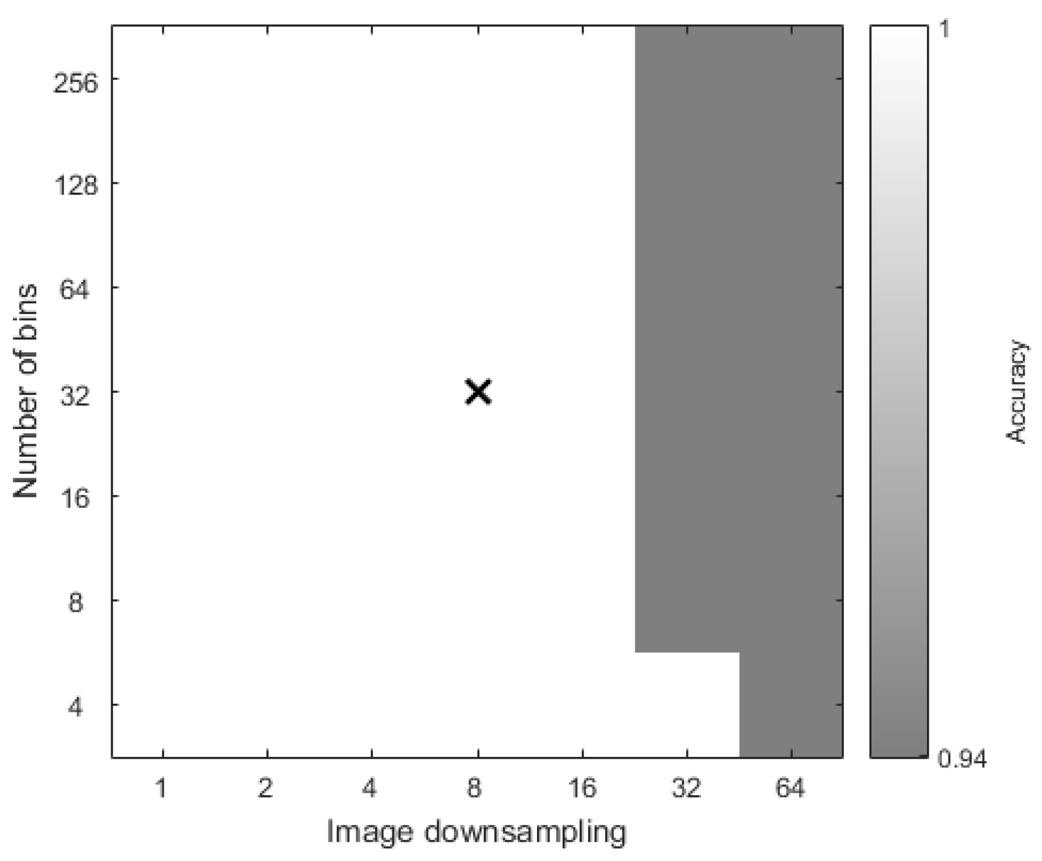
3.1. Illumination Classification

The proposed illumination classification showed a high accuracy (0.94–1.0) on the training set across a large range of image scales and a number of histogram bins, as seen in Figure 7. The accuracy of the classification is independent of the number of bins, but at large downsampling factors (32 and 64), the accuracy is affected and drops to 0.94. A factor of eight for downsampling and 32 bins for the histograms were chosen, as this had an accuracy of one on the training set. Using the template histograms for each class generated from the training set to classify the illumination of the images in the test set resulted in an accuracy of one for the chosen values.

3.2. Image Segmentation

The training of the algorithm was performed as described in Section 2.2.5.

Table 2. Training results for the image segmentation. All the results shown are the percentage frequency-weighted intersection over union. The first three columns (“global”) show the results for each method, when they are trained independently of the illumination. Indirect and direct show the results for the images of the two illuminations, respectively. Both show the combination of the results from the two illuminations. The last three columns (“individual”) show the results for each method, where the two illuminations are treated separately. The highest frequency weighted intersection over union is bolded in each column.

	Global			Individual
Method	Both	Indirect	Direct	Both	Indirect	Direct
Bonesmo	40.4%	48.2%	27.5%	40.3%	48.7%	29.0%
Bonesmo + $ExG{R}_C$	40.3%	48.1%	27.4%	40.2%	48.7%	29.1%
Bonesmo + $ExG{R}_N$	42.2%	48.5%	31.4%	42.1%	49.4%	33.6%
Bonesmo + Flood-fill	38.1%	40.7%	34.1%	40.9%	46.1%	34.5%
Bonesmo + Watershed	40.8%	47.1%	30.0%	42.1%	48.6%	33.3%
Bonesmo + Watershed + Flood-fill	39.1%	46.4%	27.0%	39.6%	46.9%	31.1%
Bonesmo + $ExG{R}_C$ + Watershed	41.2%	46.8%	32.7%	42.6%	48.6%	34.8%
Bonesmo + $ExG{R}_N$ + Watershed	43.2%	47.8%	35.5%	43.7%	49.2%	37.7%
Bonesmo + $ExG{R}_C$ + Watershed + Flood-fill	39.1%	46.4%	27.0%	41.9%	46.9%	36.8%
Bonesmo + $ExG{R}_N$ + Watershed + Flood-fill	40.3%	45.0%	32.7%	41.5%	47.6%	37.7%

shows the fwIoU results of the training. As expected, training the images with indirect and direct illumination separately generally outperformed training the two illumination cases together. In all cases, the images with indirect illumination were segmented better than those with direct illumination. The largest improvements with respect to fwIoU were seen on the images with direct illumination. Most improvements resulted in an increased fwIoU with the exception of the methods with flood-filling, when compared to the counterparts without flood-filling.

Using the normalized RGB values for calculating $ExGR$ performed better than using the chromaticity. Using the chromaticity often resulted in little to no improvement when compared to not using $ExGR$, whereas using the normalized RGB values gave higher fwIoU in all cases except one.

$ExG{R}_N$ had the biggest impact on performance, as it reduced the amount of soil classified as clover and grass. However, an increase in grass classified as soil was seen. Watershed also had a great impact on the performance; mainly when the images from the two illuminations were trained separately.

Using flood-fill to recreate the clover leaves rather than morphological dilation had a negative impact on the overall result in most cases when compared to using no improvements. The performance on the indirect illumination images decreased compared to simply using dilation; however, the performance on the direct illumination images increased. Combining Bonesmo with $ExG{R}_N$ and watershed was the best performing method on our training set with respect to both training the images from the two illuminations together and separately. The latter performed slightly better than the former, and it was therefore selected for segmenting the images and calculating the clover and grass coverage used in the dry matter estimation. Evaluating Bonesmo + $ExG{R}_N$ + watershed on the test set yielded a 39.0% fwIoU.

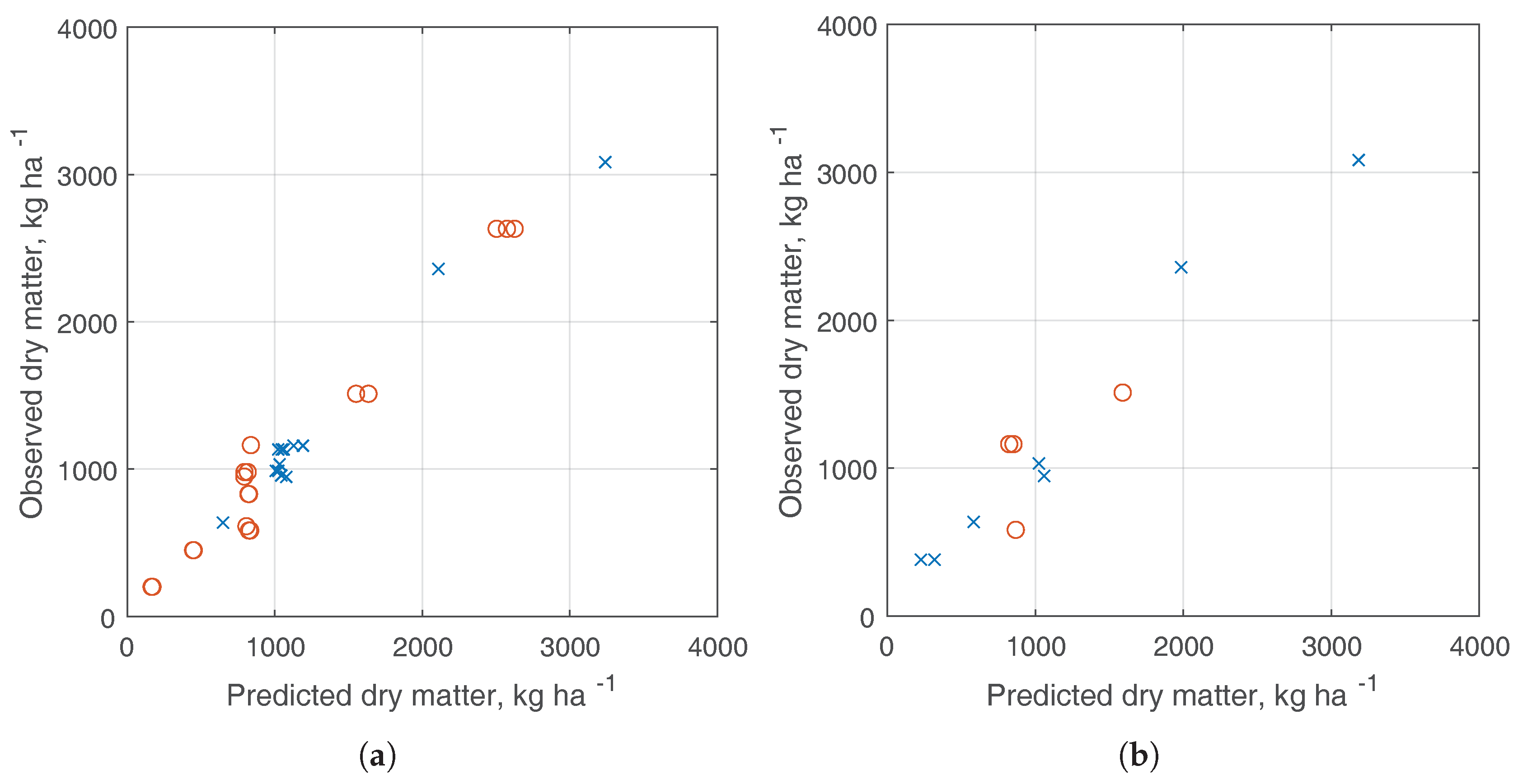
3.3. Dry Matter Estimation

The total dry matter model was trained using stepwise linear regression with a strictly linear model as the initial model. Terms were added and removed based on their significance. During training, significant interactions between the accumulated sunshine hours and temperature sum since last harvest and between the accumulated sunshine and mixture were found. After adding these terms, the clover coverage was no longer significant, and it was removed. The final model was:

$$DM={\beta }_0+{\beta }_1{C}_G+{\beta }_{3}S+{\beta }_{4}T+{\beta }_{5}M+{\beta }_{6}ST+{\beta }_{7}SM$$

(7)

where $DM$ was the total dry matter, $C_G$ is the grass coverage, respectively, S is the accumulated sunshine hours since last harvest, T is the temperature sum since last harvest, M is a categorical variable describing the mixture (“Mixture 35” or “Mixture 45”) and ${\beta }_{0–7}$ are the weights of each term. The values of the weights for each variable, as well as their significance are shown in

Table 3. Estimated variable weights for the final total dry matter model. $C_G$ is the Clover Coverage. S is the accumulated Sunshine hours since last harvest. T is the Temperature sum since last harvest. M is a factor variable describing the Mixture. SE is the Standard Error. t is the t-statistic for a test for which the coefficient is zero. p is the p-value for the t-statistic (stepwise linear regression (stepwiselm) in MATLAB [32]).

Variable	Estimate	SE	t	p
Intercept	−205	884	−0.242	0.810
$C_G$	845	389	2.17	0.0390
S	−0.585	6.40	−0.0915	0.928
T	−0.147	0.0790	−1.86	0.0739
M	409	233	1.76	0.0901
S:T	0.00181	0.000611	2.96	0.00636
S:M	−3.98	1.4	−2.84	0.000848

. As seen, all terms were significant with the exception of the intercept and the accumulated sunshine hours. However, the accumulated sunshine hours had significant interactions with both the temperature sum since last harvest and the mixture. The total dry matter was dependent on the mixture. In particular, “Mixture 45” further added an additional 409 kg ha${}^{-1}$ of dry matter compared to “Mixture 35”. Correlation plots between the predicted and observed dry matter of the training ($R^2=0.97$) and test set ($R^2=0.93$) show a high correlation and no clear outliers (Figure 8). The error measures of the final dry matter model are shown in

Table 4. Error measures for the total dry matter model. The error measures are the Root Mean Square Error (RMSE), Normalized RMSE (NRMSE), the Mean Absolute Error (MAE) and the Mean Absolute Relative Error (MARE) for the training and test sets.

Dataset	RMSE	NRMSE	MAE	MARE
Training set	125 kg ha${}^{-1}$	11%	90 kg ha${}^{-1}$	9.8%
Test set	210 kg ha${}^{-1}$	17.5%	171 kg ha${}^{-1}$	19%

.

4. Discussion

The proposed improvements to the image segmentation algorithm initially proposed by Bonesmo et al. [6] increased the frequency-weighted intersection over union. The only exception was the reconstruction of clover leaves by looking up the remaining segments in the segmented image prior to the erosions. This was likely due to it being very dependent on correct edge detection. If the edge between two adjacent clover and grass leaves were not detected, dilating the segment would reconstruct the clover leaf and part of the grass leaf, while looking up the original segment would reconstruct the entire clover and grass leaf, resulting in a lower intersection over union. In contrast to the general picture, the segmentation of the images captured under the direct illumination improved when using the flood-filling method. This is likely due to the large image gradients between parts of leaves in shadow and non-shadow. This created some easily detectable edges while still retaining relatively large clover segments compared to the grass segments. As seen in Figure 1b, the captured images contains several white clover seed heads. The clover seed heads were not handled explicitly, and due to their color, they were mainly misclassified as soil/dead plants.

The captured images were stored in JPG-format, which is a lossy file-format. The overall structure of the scene is still captured, but finer details such as edges may be lost during compression. This is particularly harmful in methods such as the proposed, which rely heavily on detecting edges between objects. Storing the captured images in a lossless format could mitigate this problem.

Overall, the image segmentation method has very few degrees of freedom for capturing the variability of the images. In the future, higher capacity methods such as texture analysis [23,33] or self-taught features in deep convolutional neural networks [28,29] might be a better option for achieving higher accuracy and intersection over union. However, these methods require large amounts of annotated data to be trained.

In the final dry matter model, the clover coverage was not significant and was therefore excluded. This is explained by the close relationship between the clover and grass coverages in the dataset, which can be expressed as:

$$C_C\approx 1-C_G$$

(8)

Inserting this into Equation (6), the clover coverage vanishes, and the model is reduced to Equation (7) excluding the interactions. Thus, the clover coverage is implicitly expressed in the intercept term and the grass coverage term.

The proposed illumination classification for model parameter selection was able to distinguish between the two classifications with a high accuracy. However, it is rather awkward to have an illumination model with only two classes, since illumination is generally a continuous function. Therefore, the algorithm should ideally be independent of illuminations, as well as image resolution and pixel density, to make it as generally applicable as possible. An alternative solution would be to control the illumination while capturing the images to ensure a more even illumination across the images [34,35].

The 210-kg ha${}^{-1}$ biomass RMSE on the test set on a biomass range from 195–3084 kg ha${}^{-1}$ biomass is highly acceptable for the farmers. However, the model should be tested in fields with higher biomass yields, as well as on a larger dataset. In contract, the GrazeGro growth model has an RMSE of 9.9–64.5 kg dry matter ha${}^{-1}$ day${}^{-1}$ depending on the dataset [3]. The NRMSE of 11–17.5% for the proposed model is comparable to that reported for the CATIMO model for both timothy-grass (NRMSE = 15–25%) [10] and meadow bromegrass (NRMSE = 16–39%) [11]. The proposed model covers two very distinct clover-grass mixtures widely used in Danish agriculture. We would therefore expect similar high correlations and low RMSE if more national clover-grass mixtures were included in the model, as they differ only slightly in their clover/grass composition. On the other hand, we would expect lower correlation and higher RMSE if foreign clover-grass mixtures were included in the model. We strongly believe in a future scenario where images are captured during field operations together with already collected climate parameters and field history, including current clover-grass mixture. This will give valuable information of biomass production and thereby forage production and important information to increase nutrient utilization. Especially, the ratio between clover and grass is important for N application due to competition between the two crop species for N. The combination of a high grass share and high N application will inevitably outcompete the clover crop and consequently lower the protein production in the field [36]. On the other hand, a high clover ration in combination with low N application will outcompete the grass crop and consequently the carbohydrate production in the field [36]. Being able to adjust the N application in a clover-grass field will undoubtedly have a large impact on the farmer’s net-revenue, but also on the environmental impact due to N application geared toward the clover-grass ratio.

The proposed method has been softly validated on a test set extracted from the same dataset as the training set. Therefore, some correlation between the two is expected despite only using the test set for validation. As with any proper method validation, the belief in the proposed method would benefit from a hard validation on a completely independent test set based on recordings from a different year at a different location.

5. Conclusions

The preliminary results presented in this paper strongly indicate that total clover-grass dry matter can be estimated using grass coverage derived from image analysis along with climate parameters. The estimated total dry matter could be used in conjunction with current state-of-the-art image analysis methods for estimating the dry matter contribution of clover [7].

The applied image analysis method was developed by Bonesmo et al. [6], but three improvements were proposed and evaluated along with the original method. Two of the three proposed improvements ($ExGR$ and watershed) increased performance with respect to the fwIoU. The third improvement (reconstruction using the original blob) did not increase the fwIoU due to imperfect edge detection between the leaves. Grouping the images based on their illumination (direct and indirect sunlight) and training each group independently further improved the fwIoU. The grouping was performed using a novel approach based on a histogram of $ExGR$ compared to two reference histograms.

References

1. Søegaard, K. Nitrogen fertilization of grass/clover swards under cutting or grazing by dairy cows. Acta Agric. Scand. Sect. B 2009, 59, 139–150. [Google Scholar]
2. Kuoppala, K. Influence of Harvesting Strategy on Nutrient Supply and Production of Dairy Cows Consuming Diets Based on Grass and Red Clover Silage. Ph.D. Thesis, Department of Agricultural Sciences, University Helsinki, Helsinki, Finland, 2010. [Google Scholar]
3. Barrett, P.; Laidlaw, A.; Mayne, C. GrazeGro: A European herbage growth model to predict pasture production in perennial ryegrass swards for decision support. Eur. J. Agron. 2005, 23, 37–56. [Google Scholar] [CrossRef]
4. Biewer, S.; Erasmi, S.; Fricke, T.; Wachendorf, M. Prediction of yield and the contribution of legumes in legume-grass mixtures using field spectrometry. Precis. Agric. 2009, 10, 128–144. [Google Scholar] [CrossRef]
5. Friedl, M.A.; Schimel, D.S.; Michaelsen, J.; Davis, F.W.; Walker, H. Estimating grassland biomass and leaf area index using ground and satellite data. Int. J. Remote Sens. 1994, 15, 1401–1420. [Google Scholar] [CrossRef]
6. Bonesmo, H.; Kaspersen, K.; Kjersti Bakken, A. Evaluating an image analysis system for mapping white clover pastures. Acta Agric. Scand. Sect. B 2004, 54, 76–82. [Google Scholar] [CrossRef]
7. Himstedt, M.; Fricke, T.; Wachendorf, M. The benefit of color information in digital image analysis for the estimation of legume contribution in legume-grass mixtures. Crop Sci. 2012, 52, 943–950. [Google Scholar] [CrossRef]
8. McRoberts, K.C.; Benson, B.M.; Mudrak, E.L.; Parsons, D.; Cherney, D.J. Application of local binary patterns in digital images to estimate botanical composition in mixed alfalfa–grass fields. Comput. Electron. Agric. 2016, 123, 95–103. [Google Scholar] [CrossRef]
9. Schapendonk, A.; Stol, W.; van Kraalingen, D.; Bouman, B. LINGRA, a sink/source model to simulate grassland productivity in Europe. Eur. J. Agron. 1998, 9, 87–100. [Google Scholar] [CrossRef]
10. Jing, Q.; Bélanger, G.; Baron, V.; Bonesmo, H.; Virkajärvi, P.; Young, D. Regrowth simulation of the perennial grass timothy. Ecol. Model. 2012, 232, 64–77. [Google Scholar] [CrossRef]
11. Bonesmo, H.; Baron, V.S.; Young, D.; Bélanger, G.; Jing, Q. Adapting the CATIMO grass model to meadow bromegrass grown in western Canada. Can. J. Plant Sci. 2014, 94, 61–71. [Google Scholar] [CrossRef]
12. Adam, E.; Mutanga, O.; Rugege, D. Multispectral and hyperspectral remote sensing for identification and mapping of wetland vegetation: A review. Wetl. Ecol. Manag. 2010, 18, 281–296. [Google Scholar] [CrossRef]
13. Xie, Y.; Sha, Z.; Yu, M. Remote sensing imagery in vegetation mapping: A review. J. Plant Ecol. 2008, 1, 9–23. [Google Scholar] [CrossRef]
14. Rembold, F.; Atzberger, C.; Savin, I.; Rojas, O. Using Low Resolution Satellite Imagery for Yield Prediction and Yield Anomaly Detection. Remote Sens. 2013, 5, 1704–1733. [Google Scholar] [CrossRef] [Green Version]
15. Joshi, N.; Baumann, M.; Ehammer, A.; Fensholt, R.; Grogan, K.; Hostert, P.; Jepsen, M.R.; Kuemmerle, T.; Meyfroidt, P.; Mitchard, E.T.A.; et al. A Review of the Application of Optical and Radar Remote Sensing Data Fusion to Land Use Mapping and Monitoring. Remote Sens. 2016, 8, 70. [Google Scholar] [CrossRef]
16. Lefsky, M.A.; Cohen, W.B.; Parker, G.G.; Harding, D.J. Lidar Remote Sensing for Ecosystem StudiesLidar, an emerging remote sensing technology that directly measures the three-dimensional distribution of plant canopies, can accurately estimate vegetation structural attributes and should be of particular interest to forest, landscape, and global ecologists. Bioscience 2002, 52, 19–30. [Google Scholar]
17. Ju, J.; Roy, D.P. The availability of cloud-free Landsat ETM+ data over the conterminous United States and globally. Remote Sens. Environ. 2008, 112, 1196–1211. [Google Scholar] [CrossRef]
18. Åstrand, B.; Baerveldt, A.J. An agricultural mobile robot with vision-based perception for mechanical weed control. Auton. Robot. 2002, 13, 21–35. [Google Scholar] [CrossRef]
19. Giselsson, T.M.; Midtiby, H.S.; Jørgensen, R.N. Seedling discrimination with shape features derived from a distance transform. Sensors 2013, 13, 5585–5602. [Google Scholar] [CrossRef] [PubMed] [Green Version]
20. Dyrmann, M.; Christiansen, P. Automated Classification of Seedlings Using Computer Vision; Aarhus University: Aarhus, Denmark, 2014. [Google Scholar]
21. McCarthy, C.L.; Hancock, N.H.; Raine, S.R. Applied machine vision of plants: A review with implications for field deployment in automated farming operations. Intell. Serv. Robot. 2010, 3, 209–217. [Google Scholar] [CrossRef] [Green Version]
22. Gebhardt, S.; Schellberg, J.; Lock, R.; Kühbauch, W. Identification of broad-leaved dock (Rumex obtusifolius L.) on grassland by means of digital image processing. Precis. Agric. 2006, 7, 165–178. [Google Scholar] [CrossRef]
23. Gebhardt, S.; Kühbauch, W. A new algorithm for automatic Rumex obtusifolius detection in digital images using colour and texture features and the influence of image resolution. Precis. Agric. 2007, 8, 1–13. [Google Scholar] [CrossRef]
24. Krizhevsky, A.; Sutskever, I.; Hinton, G.E. Imagenet classification with deep convolutional neural networks. In Proceedings of the Advances in Neural Information Processing Systems, Lake Tahoe, NV, USA, 3–6 December 2012; pp. 1097–1105. [Google Scholar]
25. Szegedy, C.; Liu, W.; Jia, Y.; Sermanet, P.; Reed, S.; Anguelov, D.; Erhan, D.; Vanhoucke, V.; Rabinovich, A. Going deeper with convolutions. In Proceedings of the IEEE Conference on Computer Vision and Pattern Recognition, Boston, MA, USA, 7–12 June 2015; pp. 1–9. [Google Scholar]
26. Long, J.; Shelhamer, E.; Darrell, T. Fully convolutional networks for semantic segmentation. In Proceedings of the IEEE Conference on Computer Vision and Pattern Recognition, Boston, MA, USA, 7–12 June 2015; pp. 3431–3440. [Google Scholar]
27. Ronneberger, O.; Fischer, P.; Brox, T. U-Net: Convolutional Networks for Biomedical Image Segmentation. Proceedings of Medical Image Computing and Computer-Assisted Intervention, Munich, Germany, 5–9 October 2015; Springer; pp. 234–241. [Google Scholar]
28. Mortensen, A.K.; Dyrmann, M.; Karstoft, H.; Jørgensen, R.N.; Gislum, R. Semantic Segmentation of Mixed Crops using Deep Convolutional Neural Network. In Proceedings of the International Conference on Agricultural Engineering 2016, Aarhus, Danmark, 26–29 June 2016. [Google Scholar]
29. Dyrmann, M.; Mortensen, A.K.; Midtiby, H.S.; Jørgensen, R.N. Pixel-wise classification of weeds and crop in images by using a Fully Convolutional neural network. In Proceedings of the International Conference on Agricultural Engineering 2016, Aarhus, Danmark, 26–29 June 2016. [Google Scholar]
30. Meyer, G.E.; Neto, J.C. Verification of color vegetation indices for automated crop imaging applications. Comput. Electron. Agric. 2008, 63, 282–293. [Google Scholar] [CrossRef]
31. Beucher, S.; Lantuéjoul, C. Use of Watersheds in Contour Detection. In Proceedings of the International Workshop on Image Processing: Real-Time Edge and Motion Detection/Estimation, Rennes, France, 17–21 September 1979. [Google Scholar]
32. MATLAB R2015a (8.5.0); The MathWorks Inc.: Natick, MA, USA, 2015.
33. Mortensen, A.K.; Gislum, R.; Larsen, R.; Nyholm Jørgensen, R. Estimation of above-ground dry matter and nitrogen uptake in catch crops using images acquired from an octocopter. In Proceedings of the 10th European Conference on Precision Agriculture, Volcani Center, Israel, 12–16 July 2015; pp. 127–134. [Google Scholar]
34. Jensen, K.; Laursen, M.S.; Midtiby, H.; Jørgensen, R.N. Autonomous Precision Spraying Trials Using a Novel Cell Spray Implement Mounted on an Armadillo Tool Carrier. In Proceedings of the XXXV CIOSTA & CIGR V Conference, Billund, Denmark, 3–5 July 2013. [Google Scholar]
35. Overskeid, O.; Hoeg, A.; Overeng, S.; Stavlund, H. System for Controlled Application of Herbicides. U.S. Patent 8,454,245, 4 June 2013. [Google Scholar]
36. Harris, S.L.; Thom, E.R.; Clark, D.A. Effect of high rates of nitrogen fertiliser on perennial ryegrass growth and morphology in grazed dairy pasture in northern New Zealand. N. Z. J. Agric. Res. 1996, 39, 159–169. [Google Scholar] [CrossRef]
Figure 1. (a) Photo of how the images were captured. The digital camera was mounted on the end of the pole and facing down. (b) Example of captured image covering approximately 80 × 100 cm 2 .
Jimaging 03 00059 g001
Figure 2. Patches extracted from the image captured in direct (a) and indirect (c) sunlight and the corresponding annotated image patches (b) and (d), respectively.
Jimaging 03 00059 g002
Figure 3. Overview of the image segmentation method and proposed improvements. The block diagram shows the steps involved in the soil-clover-grass segmentation of the image. Above each block, the method used by Bonesmo et al. [6] is shown. Below each block, our proposed alternatives are shown. To distinguishing between soil and green plant material, Bonesmo et al. [6] used the ratio between green and red ( g / ( r + 1 ) ), where we propose to use the difference between excess green and excess red ( E x G - E x R ). Next, grass and clover are distinguished in three steps. In the first step, edges are detected. Bonesmo et al. [6] thresholded a gradient image derived from the Sobel operator to detect edges. We propose using the watershed algorithm to derive the edges from the gradient image. In the second step, grass is removed by morphologically eroding the inverted edge image. In the third step, clover is reconstructed. Here, Bonesmo et al. [6] used morphological dilation. We propose using flood filling of the inverted edge image to reconstruct the clover leaves. All pixels not reconstructed are regarded as grass.
Jimaging 03 00059 g003
Figure 4. Example of clover and grass segmentation using the original method proposed by Bonesmo et al. [6]. (a) Original image captured in indirect sunlight; (b) soil green-red ratio image; (c) threshold soil image; (d) Sobel gradient image; (e) edge image; (f) segmented image prior to erosion; (g) segmented image after the erosions; (h) reconstructed clover image using dilation; (i) grass image; (j) classification image. Yellow = grass. Purple = clover. Red = soil/dead plants.
Jimaging 03 00059 g004
Figure 5. Example of clover and grass segmentation using the proposed improvements. (a) Original image captured in indirect sunlight; (b) soil E x G R N image; (c) threshold soil image; (d) gradient of blurred image; (e) edge image using watershed; (f) segmented image prior to erosion; (g) segmented image after the erosions; (h) reconstructed clover image using flood-filling; (i) grass image; (j) classification image. Yellow = grass. Purple = clover. Red = soil/dead plants.
Jimaging 03 00059 g005
Figure 6. Example of illumination histograms using 32 bins and a factor of 8 downscaling of the images. Example of histograms of images from the test set for the two illuminations using the selected settings (bin size of 32 and a factor of 8 downsampling of the images), as well as the corresponding templates generated from the training set.
Jimaging 03 00059 g006
Figure 7. Accuracy as a function of the number of bins in the histogram and the downsampling of the image based on the image training set. The bold × indicates the selected optimal settings.
Jimaging 03 00059 g007
Figure 8. Correlation plots of predicted and observed total dry matter for the training set (a) and test set (b). The cross and circles indicate the two different seed mixtures used.
Jimaging 03 00059 g008