Supervised Learning to Predict Sperm Sorting by Magnetophoresis

School of Mechanical and Aerospace Engineering, Nanyang Technological University, Singapore 639798, Singapore
*
Author to whom correspondence should be addressed.
Magnetochemistry 2018, 4(3), 31; https://doi.org/10.3390/magnetochemistry4030031
Submission received: 10 May 2018
/
Revised: 12 June 2018
/
Accepted: 25 June 2018
/
Published: 2 July 2018
(This article belongs to the Special Issue Magnetic Fields in Microfluidic Systems)
Abstract
:Machine learning is gaining popularity in the commercial world, but its benefits are yet to be well-utilised by many in the microfluidics community. There is immense potential in bridging the gap between applied engineering and artificial intelligence as well as statistics. We illustrate this by a case study investigating the sorting of sperm cells for assisted reproduction. Slender body theory (SBT) is applied to compute the behavior of sperm subjected to magnetophoresis, with due consideration given to statistical variations. By performing computations on a small subset of the generated data, we train an ensemble of four supervised learning algorithms and use it to make predictions on the velocity of each sperm. Our results suggest that magnetophoresis can magnify the difference between normal and abnormal cells, such that a sorted sample has over twice the proportion of desirable cells. In addition, we demonstrated that the predictions from machine learning gave comparable results with significantly lower computational costs.
1. Introduction
The World Health Organisation (2002) found that about one in ten couples worldwide experience difficulties conceiving. Today, assisted reproduction techniques account for over 1% of the infants born in developed countries [1].
The chances of successful conception significantly dependent on sperm morphology, both in natural fertilisation [2] as well as the various forms of assisted reproduction ([3,4,5]). Hence, it is beneficial to come up with sorting procedures which improve the proportion of such sperm in a sample. While desirable sperm cells can be manually selected for use in in-vitro fertilisation (IVF) or intracytoplasmic sperm injection (ICSI) [6], this is not feasible for intrauterine insemination (IUI) given the large number of sperm required. Therefore, the procedure should ideally be passive.
There are a variety of methods [7] to sort human sperm cells by their motility or morphology, as well as a multitude of microfluidic techniques yet to be used on sperm cells [8,9,10]. Dielectrophoresis [11] has been applied to separate mature spermatozoa from non-mature spermatogenic cells [12]. A separate group of researchers performed magnetic-activated cell sorting to obtain viable and morphologically normal spermatozoa that enjoy higher cryosurvival rates [13,14]. A magnetic particle in diamagnetic medium experiences a magnetic force towards the region of higher magnetic field density, while the opposite is true for a diamagnetic particle in paramagnetic medium [15]. Therefore, the sperm cells may be doped with paramagnetic nanoparticles [16] or sorted in their natural form via diamagnetophoresis [17]. Despite evidence that sperm cells subjected to a magnetic field remain viable with the potential for fertilisation [16,18], there is more to be studied before such sorted spermatozoa may be used to increase the success rates of assisted reproduction for the public.
Due to ethical concerns involved in carrying out experiments with human sperm, it is beneficial for researchers to first carry out theoretical studies to assess the feasibility of sorting using the various techniques under different experimental set-ups. Mathematical models of increasing complexity and accuracy have been developed to understand the kinematics of micro-swimmers such as sperm cells [19,20]. These theoretical computations are often taken from the deterministic approach. However, as sperm cells differ in their morphology, more insights can be gained by studying their behavior from a statistical approach.
In spite of technological advances, precise theoretical models are still computationally expensive, and running numerical simulations for a large number of samples to obtain statistically reliable results may be time-consuming. Moreover, in the process of testing for convergence, the scale of simulations that are carried out will exceed that which is required for statistical analysis. Notably, the use of machine learning [21] has been proven to provide accurate predictions and is gaining popularity, but its use in engineering research is still not widespread despite great potential. Common models include k-nearest neighbor regression [22], ridge regression [23], random forest regression [24], and artificial neural networks [25]. In k-nearest neighbor regression, the predictor and target variables of all known samples are stored. For all new data to be predicted, only the k samples having the least ‘distance’ will be considered, with the simple or weighted-average value taken. Ridge regression is linear regression with L2 regularization, where a penalty term is added to the sum of square errors to be minimized, thus avoiding overly-large coefficients in the linear model. In random forest regression, a large number of decision trees is built, each using a subset of predictor variables so as to avoid overfitting. For each decision tree, the population is split based on one variable at a time, where the chosen variable as well as threshold determining the split minimizes the sum of square errors (in the case of regression). In artificial neural networks, the first layer or nodes receives input from the predictor variables, adds a bias to the weighted sum and passes it through a non-linear function, and feeds the output to the subsequent layer of nodes. This continues until an output is obtained from the final single node after the hidden layer. The weights and bias are ‘learnt’ by minimizing the cost function via optimization. Each model has its own hyperparameters to be tuned, and there are also other well-established supervised learning algorithms, but the four mentioned above will suffice for the scope of this paper. There is no single best learning algorithm [26], and therefore ensembles often out-perform [27] their individual components. In this paper, we will apply supervised learning using an ensemble of the aforementioned algorithms.
Slender body theory (SBT) will be used to to compute the kinematic behavior of spermatozoa, with two goals in mind. Statistical analysis will be carried out with varying amounts of data, to find out the quantity of data which is sufficient without being excessive. This will be explored by studying the sorting of spermatozoa via magnetophoresis to enhance the proportion of morphologically normal cells. Secondly, we explore the feasibility of using machine learning on a smaller dataset to predict the results, so as to save computational or laboratory costs. Our findings can be generalised to other theoretical simulations utilising a different model to compute the hydrodynamics of some organism, as well as to experimenters obtaining actual data.
2. Model
A human sperm has a head of length lh = 4.81 ± 0.43 µm and width wh = 3.32 ± 0.38 µm [28], with a typical thickness gh of 1.1 µm [29]. Attached to the head is a flagellum of arc length Λ = 42 ± 4 µm [30] with a radius of 0.25 µm [31]. The flagellar beat frequency f and amplitude b also vary [32] according to the sperm head morphology. The swimming speed of a human sperm ranges from 36 to 51 µm s−1 [32]. Under such small length and velocity scales, the hydrodynamics of human sperms are governed by the Stokes equation. Therefore, we adopt the SBT to solve the velocity of the sperm subjected to an external magnetic field. The use of SBT significantly reduces the computational cost as compared to other numerical methods [33], at the same time providing accurate computation results which have been experimentally verified [34,35].
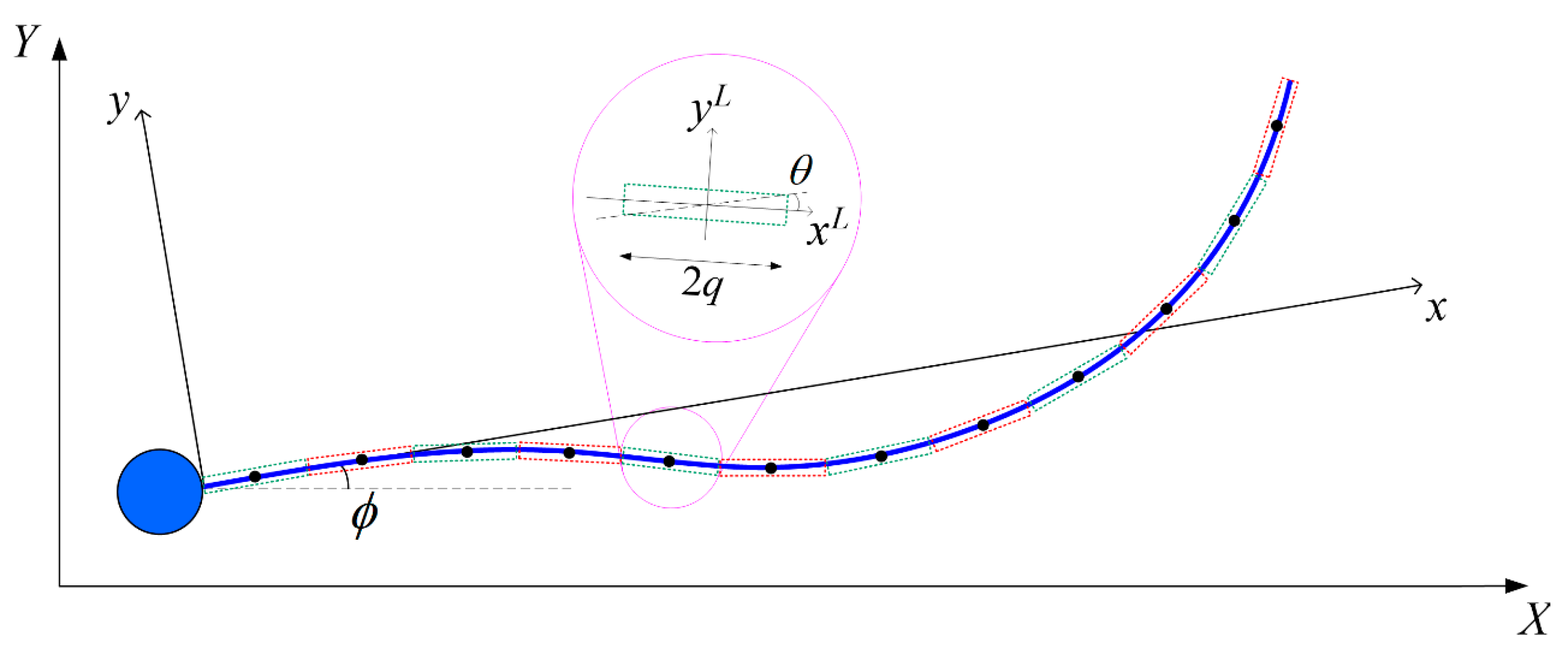
The sperm head is modelled as a sphere of radius with a volume equivalent to the ellipsoid. The origin of the body-fixed frame is located at the point where the flagellum is attached to the sperm head (Figure 1). Given that the motion of a human sperm is highly directional [36], we prescribe the flagellum beating pattern to be a modified sinusoidal waveform [37]. The centerline of the flagellum in the body-fixed frame xc = [x(t), y(x,t), z(x,t)]T has a spatial and time dependence of
where t is the time and x is the axial coordinate. The exponential term in Equation (1) ensures that the prescribed flagellum is attached to the sperm head with no deflection at the fixed end. kE controls the tapering [38] of the flagellum and is chosen to be 1/4 which gives a fair depiction of the actual sperm beating pattern [39]. At each time frame, the axial length xf(t) ends at a different value to satisfy the constraint .
SBT approximates the hydrodynamic force acting on the flagellum of arc length and radius p as that due to a series of Stokeslets and potential dipoles along its centreline [40,41]. The flagellum is discretized into N cylindrical segments, each of length 2q where p << q << Λ, with a constant force per unit length f exerted by each element on the fluid [42]. Following the conventions in Appendix A, we express the velocity at the centre of the α-th segment in the body-fixed frame uα due to the hydrodynamic force per unit length fβ exerted by the β-th segment (α, β = 1, 2, …, N) as:
The flagellum segment velocity uα can also be expressed in terms of the linear and rotational velocities, uh and ωh, of the head centre in the body-fixed frame together with the beating of the flagellum,
where εijk is the permutation symbol, rα is the displacement vector from the head centre to the centre of the α-th segment in the body-fixed frame, and vα = ∂xc/∂t is evaluated at the centre of the α-th segment. The driving force of the flagellum is provided by the relative fluid velocity it experiences due to its beating, according to the kinematics prescribed in Equation (1). This is related to the time-rate of change of the flagellum waveform, ∂y(x,t)/∂t, which is incorporated in Equation (3) under . Combining Equations (2) and (3) provides a relation between the sperm velocity and the hydrodynamic force.
We further neglect the interaction between the flagellum and head as this interaction is found to be insignificant [35,43], and hence the hydrodynamic force and moment exerted by the fluid on the head centre in the body-fixed frame are and , respectively, where μ is the fluid viscosity. To transform the force and moment from the body-fixed frame to the inertia frame, we adopt a transformation matrix H which depends on the relative orientation of the two frames. Therefore, the total hydrodynamic force and moment on the sperm in the inertia frame, based on the action and reaction, can be represented as,
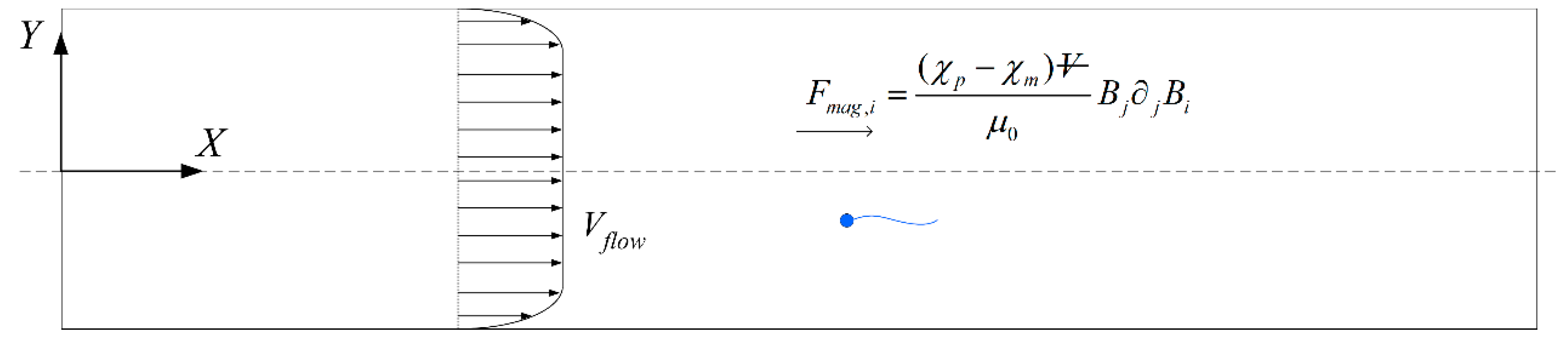
We then consider the effect of an external magnetic field to be applied for sperm sorting. A particle of volume Vp in a magnetic field B experiences the magnetic force in the inertia frame [15]:
where and are the particle and medium magnetic susceptibility, respectively, and is the magnetic permeability in vacuum. Building upon a previous work [44], we adopt the same general framework in which the magnetic field exerted on the sperm in the inertia frame satisfies the first order approximation due to the small dimension of the sperm, where C1 and C2 are constants. When O(C2X) ≪ O(C1), the magnetic force on the sperm head centre and β-th segment of the flagellum can further be simplified to and respectively, where . The total force acting on the sperm, and the total moment about the centre of the sperm head, due to the external fields can thus be represented as:
As sperm sorting is performed in the low Reynolds number regime, the total force and moment arising from the hydrodynamic propulsion and external field over the entire sperm are zero. Consider the Navier–Stokes equation in non-dimensionalised form, where Re is the Reynolds number, St the Strouhal number, p the pressure, fb the body force and the superscript tilde denotes the non-dimensionalised variable. The right side of the equation represents total force exerted on the control volume. As the Reynolds number of a swimming sperm is many orders of magnitude smaller than unity, the total force can be approximated as 0 [45], i.e., Fhydro + Fext = 0 and Mhydro + Mext = 0. Solving these equations, the instantaneous velocities of the sperm in the body-fixed frame, uh and ωh, can be obtained.
Simulations have been run on a multi-core Windows® 64bit PC (CPU E5–1650 v4, 64Gb RAM) installed with MATLAB® R2016b. An average time of 3.0 s is taken to prescribe the flagellum shape at each time frame, calculate the kernel , then to solve the instantaneous and subsequently time-averaged velocity of the sperm. This adds up to over 30 days on a single computer for every one million samples computed.
3. Results and Discussion
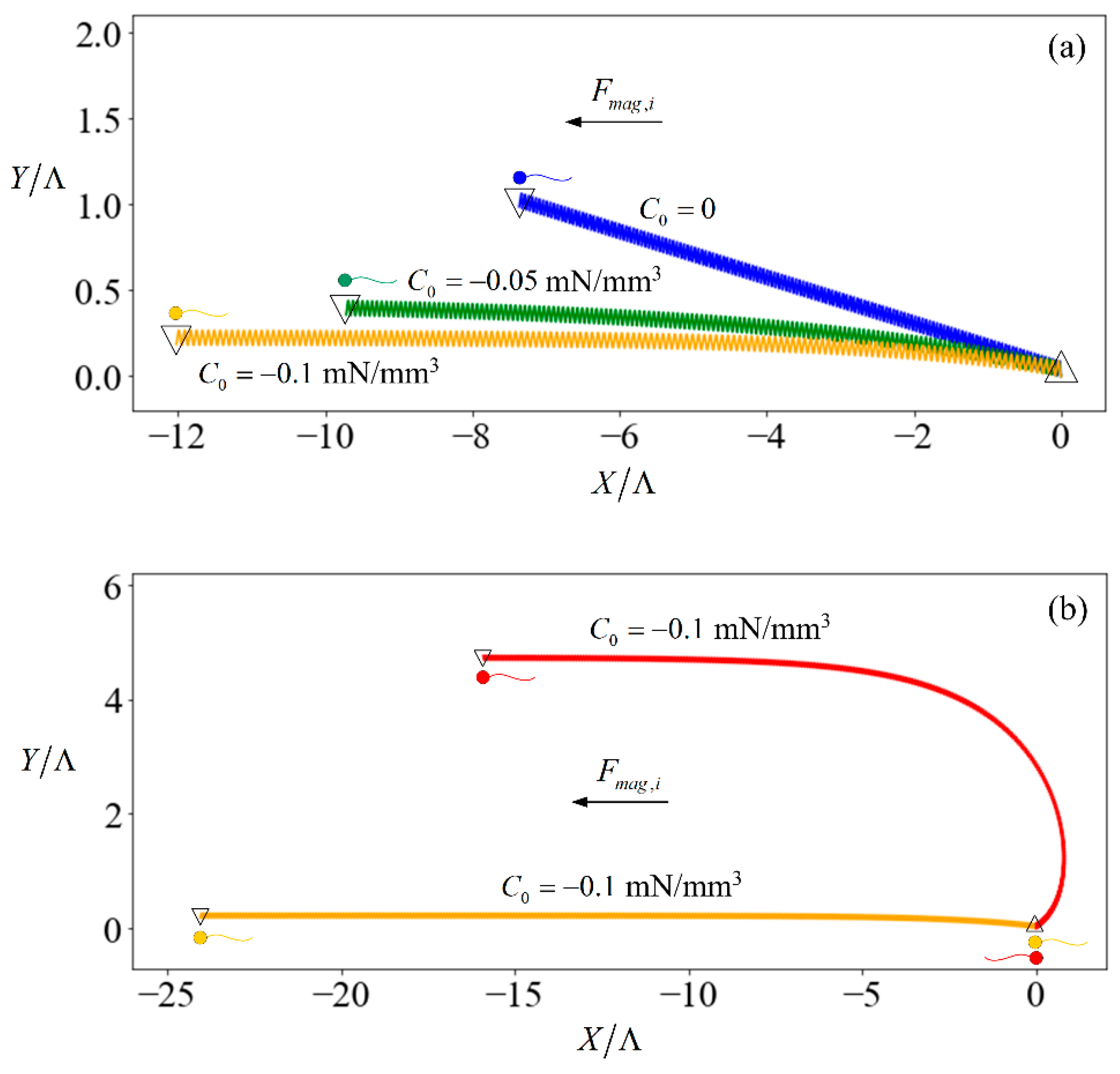
The introduction of an external force results in a stabilising effect. Figure 2a shows the trajectories of three identical sperms when subjected to no external field (trajectory denoted by blue line) versus relatively weak fields in which the induced force has the same direction as the initial heading of the sperm (trajectory denoted by yellow and green lines) for 20 s. The sperm starts off oriented along the X-axis of the inertial frame. However, the trajectory is not aligned to the X-axis due to the finite length of the flagellum. If the swimmer had been an infinite sheet [46], its motion would remain in the direction of its initial heading. The sperm flagellum motion is symmetrical over a beating cycle with respect to the x-axis in its body-frame, but asymmetrical with respect to the X-axis in the inertial frame. The instantaneous rotation of the sperm causes its orientation to change at each time instance, such that each unit of and leads to varying displacement along the X- or Y-axis of the inertial frame. The result is a net displacement in the Y-direction. A greater magnitude of C0 tends to align the sperm more strongly towards the direction where the external force is applied. This is because the larger magnetic force on the head leads to a higher time-averaged swimming velocity of the head which creates a larger hydrodynamic force to balance with the magnetic force. This difference in velocity between the head and flagellum causes the sperm to align with the external magnetic force. Therefore, our focus in the following discussion is the time-averaged velocity component of the sperm in the X-direction of the inertia frame:
For other cases that magnetic force is not in the same direction as the initial heading of the sperm; the difference in velocity between the head and flagellum tilts the sperm until it aligns with the magnetic force. To show this, we consider a scenario that the magnetic force and sperm heading are in the opposite direction (red line in Figure 2b). The magnetic force (with C0 = 0.1 mN/mm3) pulls the sperm head to the negative-X direction at a larger speed as compared to the flagellum. Consequently, the sperm aligns with the direction of the magnetic force in 20 s and continues swimming in that direction thereafter. As such, we only consider the case that the magnetic force is in the same direction as the initial heading of the sperm in the rest of the paper.
Assessment of sperm which satisfies the strict (Tygerberg) condition gives a good indication of the expected fertilisation rates [47]. Quantitatively, the sperm should have a head length of 3 to 5 µm and width of 2 to 3 µm, as well as a head width to length ratio of between three-fifths and two-thirds, with a tail measuring about 45 µm in length [48]. Without going into the biological aspects of individual sperm, a cell which fulfils these physical dimensions will be deemed conditionally satisfactory, while a cell which fails at least one condition will be considered abnormal.
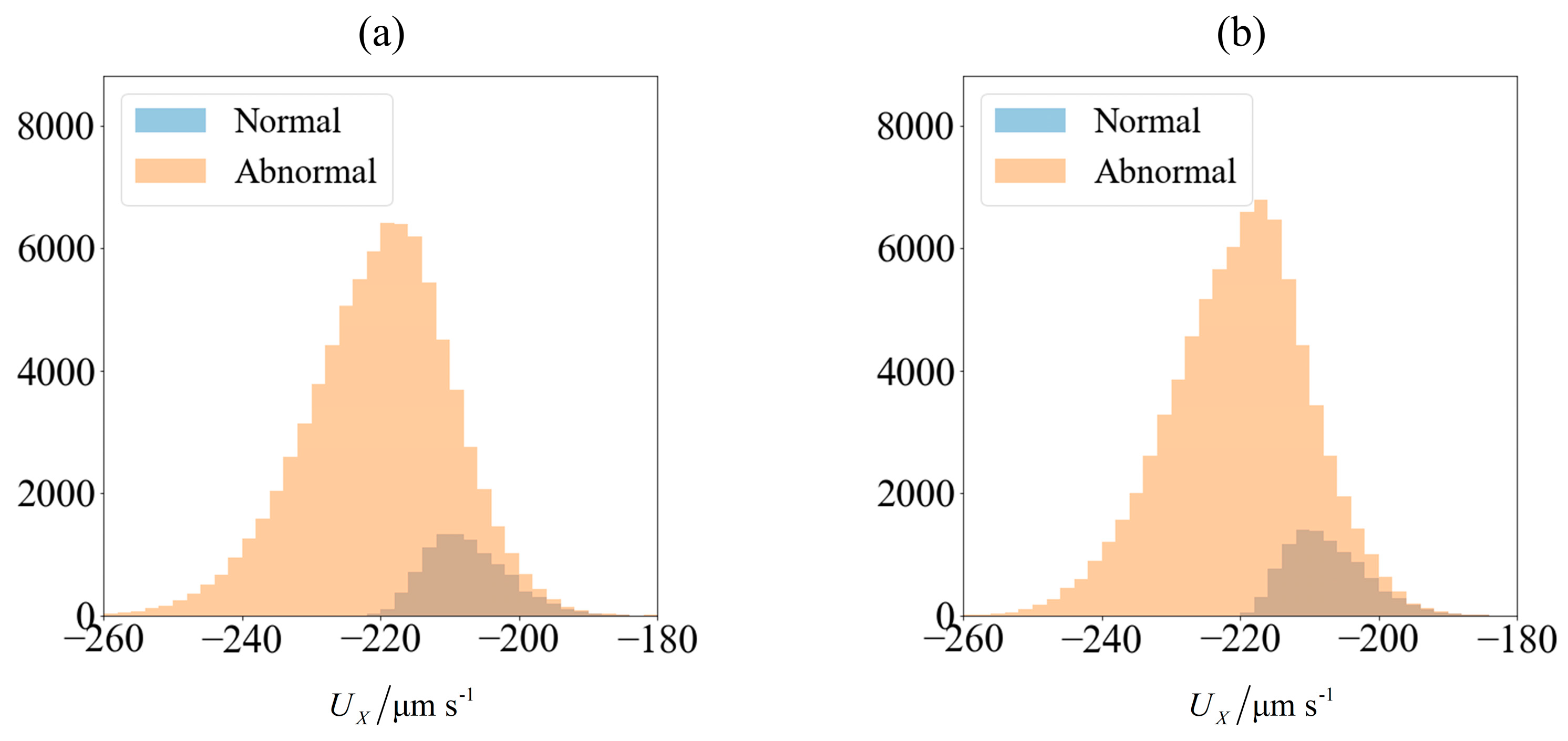
As an illustration of how the application of an external field enables sorting, we consider the velocity distribution of 100,000 sperm cells subjected to no external field (Figure 3a) and C0 = −1 mN/mm3 (Figure 4a). Using MATLAB® 2016b and setting the seed number as i for the ith sperm, a pseudo-random value is generated from Λ = 42 ± 4 μm, lh = 4.81 ± 0.43 μm and wh = 3.32 ± 0.38 μm. Each sperm is categorized based on their head morphology according to Table 1, and their flagellum beating frequency f and amplitude b are generated using the relevant mean and standard deviation. The distribution of computed velocity is presented as a histogram of normal cells super-imposed over the histogram of abnormal cells. The machine learning model is trained using 10,000 of those samples, and based on the parameters of the remaining 90,000 cells, their overall velocity distribution is predicted as shown in Figure 3b and Figure 4b. The choice of a sample size of 100,000 will be justified subsequently, as it is necessary to first introduce new parameters that will be involved in this decision.
Due to differences in the morphology as well as wriggling amplitude and frequency, the velocity distribution differs between normal and abnormal sperm. This is consistent with our previous work using resistive force theory [44]. The proportion of normal cells, as represented by the blue bars, is around 11%. This is reasonable, given that this value is reported to be 6.5 ± 3.9% [49]. One possibility of sorting cells is to introduce an opposing flow equal in magnitude to the chosen cut-off velocity. In low shear rates where the non-dimensionalised shear is in the order of , the effect of shear has insignificant influence on the flagellum waveform or sperm velocity [50]. Considering the channel width to be over an order of magnitude greater than the sperm characteristic length, the flow far from the walls acts as a bulk advection and boundary effects are negligible [44]. Cells with velocities less negative than the cut-off will acquire a net positive velocity due to advection in the positive x-direction and be eventually flushed out of the right end of the channel (Figure 5). Meanwhile, those which overcome the advection will have a net negative velocity and head towards the left end of the channel. The proportion of normal cells can be increased by modifying the cut-off velocity, but will have to come at the expense of discarding some normal cells as well. The effectiveness of sorting will be accessed according to the purity and yield as defined here:
The predicted velocities have a lower variance and tend to be distributed closer to the mean velocity, with outliers having less extreme values than what is computed (Figure 5). This is not surprising, due to the nature of the k-nearest neighbor regressor which averages out the prediction with other less extreme neighbors as well as the nature of regression trees in the random forest. Since the normal and abnormal cells are predicted to have velocities that are more tightly clustered about their respective mean values, the distinction between these two categories of sperm become magnified, leading to an optimistic estimate of the purity that can be achieved by sorting. This effect is more pronounced when a small training set is used to train the learning model, but prevails even when a large amount of data is used. Nonetheless, the qualitative conclusions from both the computed and predicted velocity distributions remain the same, that the normal sperm cells can be segregated. The extent of quantitative in the results will be explored in the following section.
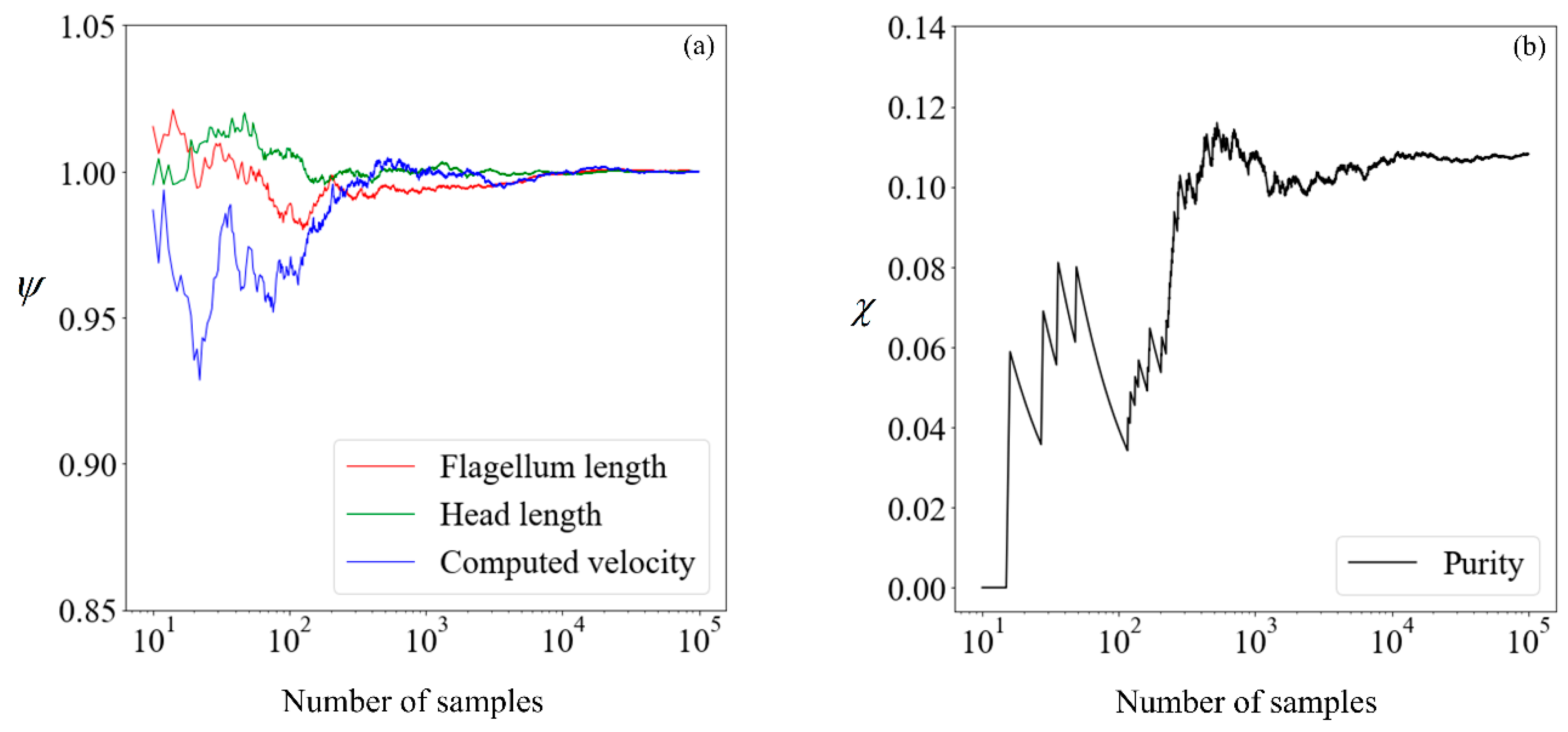
Before proceeding, it is necessary to determine the quantity of data required to obtain convergence in the results, so that a benchmark is available for subsequent comparisons. The cumulative mean flagellum length, head length, and computed velocity are presented in Figure 6, normalized with their respective mean values obtained from 100,000 samples. For the avoidance of doubt, we chose this number a posteriori, initially beginning with a small number and making increments until convergence is obtained. This normalized value is:
where n is the sample size considered, nfinal is 105, and is the sperm parameter of interest. The proportion of morphologically normal cells, which by our definition is the purity without sorting, is presented in its absolute percentage points as a function of the sample size.
Given that there are little fluctuations in all parameters when the sample size is increased from 104 to 105, we shall use the results computed using 100,000 samples as our benchmark. Moving forward, we explore the feasibility of running the simulation on a smaller number of samples and making use of supervised learning to predict the expected purity.
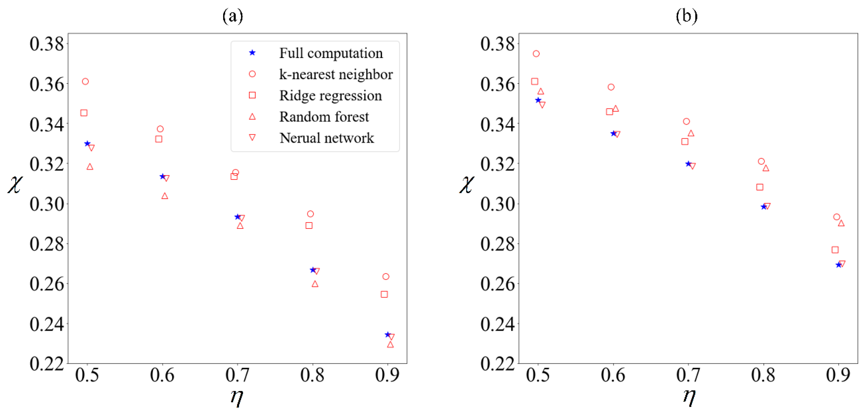
Using supervised learning algorithms from Python’s sklearn package [51], we build a supervised-learning ensemble comprising k-nearest neighbor, ridge regression, random forest regression, and artificial neural network with two hidden layers. The sperm velocity is predicted using only the following six variables as inputs; the flagellum length, the head length and width, the beating frequency and amplitude, and the applied field strength. Each cell will be classified as collected or excluded depending on its velocity distribution. The purity predicted by each algorithm trained on a tenth of the total samples is compared (Figure 7) with the purity obtained by computing the velocities of all 100,000 samples.
There are minor variations in the predictions of each algorithm, regardless of whether an external field was applied, but we have chosen not to exclude any of them from the ensemble given that none of them are outliers. Without the benefit of hindsight, it will not be known which algorithm gives a closer prediction to the ‘true’ result. Given that ensembles often out-perform [27] their individual components, we will use the mean of the predicted results henceforth.
A dataset comprising 2,100,000 rows will be obtained, where each row contains information about the sperm dimensions as well as the computed velocity under 21 different C0 values ranging from 0 to −1 mN/mm3 in intervals of 0.05 mN/mm3. This dataset will be split into training and test sets of different sizes. The test set is unused in the training process, so as to give a fair validation of the model and prevent overfitting [52].
The achievable purity corresponding to a target yield of 50% to 90% will be computed for varying magnitudes of C0. Each data point in Figure 8 is obtained by running the full computation on 105 samples, and a best-fit polynomial is added for the respective target yield. It can be observed that when the magnitude of C0 increases, the achievable purity initially decreases. This is because the normal cells generally have a higher speed than abnormal ones. Given that the abnormal sperm are generally larger than the normal ones, they are more strongly influenced when subjected to the external force. Since C0 is in the swimming direction of the sperm cells, it increases the speed of the abnormal cells to a greater extent than their normal counterparts, thereby causing the abnormal cells to catch-up. Under weak magnetophoresis, the relative shift in velocity distribution causes the two categories to become less distinct, because the abnormal sperm will be moving among the normal ones. However, increasing the strength of magnetophoresis further will increase the extent of the relative shift and eventually amplify the differences. When the magnitude of C0 increases beyond 0.9 mN/mm3, sorting can further improve the proportion of normal cells.
To assess the feasibility of sorting sperm with a magnetic force in the order of 1 mN/mm3, we consider the as described in the paragraph comprising Equation (6). Given that the magnetic susceptibility of sperm cells is similar to that of water [53], is in the order of 10−1 for sperm in non-magnetic medium, for which a very large magnetic field gradient is required to achieve mN/mm3. Hence, it may be more appropriate to dope the sperm with paramagnetic particles or use a magnetic fluid medium. For small values of and where demagnetization effects [54] can be neglected, the doping has to be limited such that has to be of order 10−1 or smaller. For mN/mm3, the minimum value of has to be 10, which can be attained using BX = 5 + 2X so that O(C2X) ≪ O(C1) in the scale of a microchannel. This corresponds to a magnetic field of 5 T, which is technically achievable [55] but its effects on the viability of sperm cells has not been reported to the best of the authors’ knowledge and remains to be verified in future experiments. To use a weaker magnetic field with a ceiling of 1.5 T [14], in which human sperm cells have been reported to remain viable in, the value of has to be of order unity. In this case, demagnetization effects will have to be considered and accounted for, and Equation (6) alone is insufficient. Here, we would like to focus on the analysis procedure using a simple model, where the objective is to introduce the framework of utilising supervised learning in microfluidic sorting. The use of magnetism for biological applications is an exciting field which warrants follow-up experimental work as well as detailed theoretical analysis, and we hope our work can provide insights and serve as a framework for future studies.
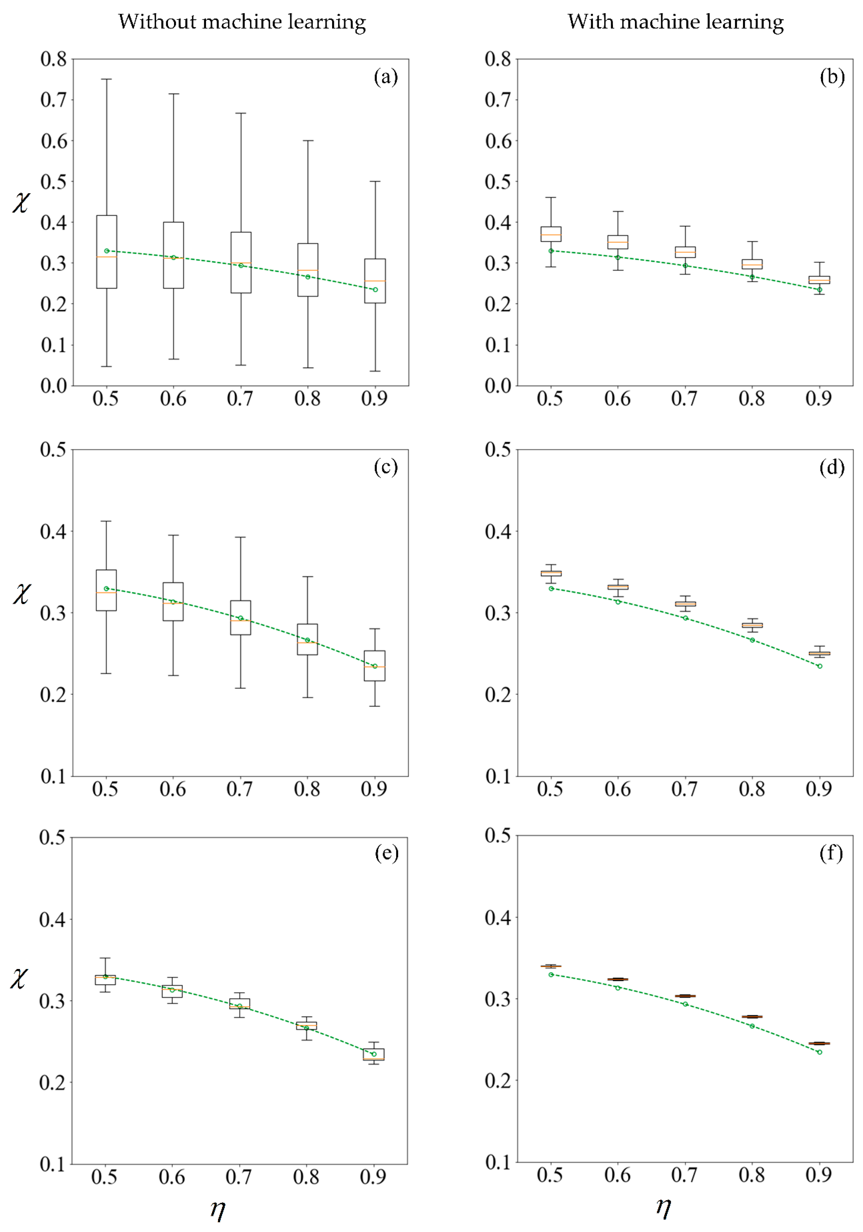
In studying non-deterministic processes such as sperm sorting, there are different approaches which may be taken (Figure 9). In this paper, we compare the results obtained by these approaches. Figure 9 compares the computed and predicted purity for a target yield of 50%, presented in box-plots, super-imposed over the best-fit polynomial for results computed using 105 samples when C0 = −1 mN/mm3. As a sample size of 105 has shown convergence, the results, as indicated by the circle markers, will be used as a benchmark. Subsets of size 100, 1000 and 10,000 are considered, by resampling with replacement [56] from the population of 100,000. Given that the variance of the results is inversely proportional to the sample size, we set the number of repetitions to be 105 divided by the size of each training set. Figure 11 shows the results under no applied field, in the same manner as described. Using the first row of Figure 10 as an illustration, a set of 100 samples is drawn to train the machine learning models. The purity using these training data are computed using the SBT model. This process is repeated 1000 times to obtain the boxplots in Figure 10a. Predictions are then made on the remaining 99,900 unseen samples, with a new machine learning model retrained for each repetition, and the results are presented in Figure 10b.
The left column of Figure 10 and Figure 11 reveals that the mean purity computed from the training data of as little as 100 samples is very close to best-fit polynomial obtained from the full computation of 105 samples. However, this is obtained from the mean of 1000 repetitions, and the large variance indicates that any individual result obtained from small sample sizes might come with a substantial error. The variance in computed purity from the training set is reduced significantly when a sample size of 10,000 is used.
In the right-hand column of Figure 10 and Figure 11, supervised learning is applied to predict the purity of all 105 samples for each C0, less those used for training, using only the six predictor variables for each sperm. Apart from the substantial reduction in variance as the number of samples in the training set increases, the error in the mean predicted purity also diminishes when the training size is increased from 100 to 10,000. Despite the consistent predictions when a training size of 10,000 is used, the mean predictions are larger for all cases considered. This is due to the phenomena where the predicted velocity distributions for each category of sperm tend to be more centered to their mean, as discussed earlier. However, there are significant savings in computational costs. After computing 10,000 samples, the time taken to train the machine learning ensemble and make predictions on the remaining 90,000 is in the order of minutes. If the velocity of those 90,000 sperm were to be computed using SBT, it would require over three days on a Windows® 64bit PC (CPU E5–1650 v4, 64Gb RAM).
Instead of running the full computation for 105 samples, one can draw the same conclusion on how sorting purity depends on yield as well as C0 by using the results predicted from one-tenth of the sample and using machine learning to make predictions on the rest. This is more reliable than solely making a conclusion from the purity of those one-tenth samples without machine learning, as evident from the shorter whiskers of each plot in the right-hand column of Figure 10 and Figure 11 as compared to their counterparts on the left. However, the improved precision obtained by machine learning comes at a cost of some reduction in accuracy, as the purity are consistently over-predicted.
We also consider the use of machine learning in investigating the sorting of sperm by dielectrophoresis, where the force is modelled as [57,58] and where is the shape factor [59] rather than volume. The conclusions drawn are similar to those above—consistent predictions with little variance are obtained when a training size of 10,000 is used—but the results are always a couple of percentage points higher than results obtained from the full computation for 105 samples.
Depending on the objectives of their study, researchers can substantially reduce computational costs by using an ensemble of a supervised machine learning model trained on a subset of the data. In cases where quantitative accuracy is important but it is not feasible to carry out experiments or the full computation on a larger scale, a number of actions may be taken. Apart from amending the predictor variables or increasing the sample size, a refined hyperparameter tuning can improve the machine learning performance, provided the training set is satisfactory. Other algorithms may also be included in the ensemble, with the weights from each constituent optimized to suit the problem at hand.
4. Conclusions
In this paper, we consider the use of magnetophoresis to sort sperm cells according to their morphology, applying SBT to compute the hydrodynamic force. Given the variations between individual sperm cells, a statistical approach is taken to study the feasibility of sorting. The mathematical procedure in SBT cannot be reduced to a straightforward analytical relation, and hence a large number of computations is required. We explore the benefit of applying machine learning to this field of microfluidics and applied engineering. An ensemble of k-nearest neighbor regression, ridge regression, random forest regression, and artificial neural network is deployed.
The results provide two key pieces of information. First, magnetophoresis influence normal and abnormal cells to different extents. Making use of the difference in their velocity distribution, the proportion of morphologically normal cells can be more than doubled through microfluidic sorting. Second, the machine learning carried out here has successfully established a reasonably accurate relation between the given sperm’s characteristics and its resulting velocity. The inference drawn from the predictions are valid qualitatively and give a good representation of the trend, using only a small fraction of the time required to run full numerical computations.
Our framework presented here will prove useful for researchers who wish to explore the feasibility of non-deterministic applications such as cell sorting. The use of machine learning enables a wider variety of possibilities to be considered, and should be embraced by fields outside computer science.
Author Contributions
J.B.Y.K. conceived the project; J.B.Y.K., X.S. and M. created the methodology; J.B.Y.K. and X.S. generated results and analyzed the data; J.B.Y.K., X.S. and M. wrote the original paper; M. supervised the team and oversaw project administration.
Funding
This research received no external funding.
Conflicts of Interest
The authors declare no conflict of interest.
Appendix A: Slender Body Theory (SBT)
Slender body theory is developed by Batchelor [41] and further applied by Lighthill [40] to solve the propulsion of microorganisms. Subsequently, Higdon [42] presented the indefinite integrals which may be applied directly without performing the integration.
The local coordinate system is set up such that the origin is located at the center of the segment of radius p and length 2q, and the xL axis coincides with the cylindrical axis (Figure 1). The velocity at any arbitrary point in the local coordinate system can be related to the hydrodynamic force per unit length fL on this segment in the local coordinate, using Equation (A1) in Higdon [42]:
When has the same component as , can be further simplified to
where .
To transfer the force and velocity from the local coordinate system to the body-fixed frame in our problem, one can use
where the transformation matrix is defined as
The velocity at any arbitrary point in the body-fixed frame can be expressed in terms of the hydrodynamic force per unit length f:
where
References
- Sutcliffe, A.G.; Ludwig, M. Outcome of assisted reproduction. Lancet 2007, 370, 351–359. [Google Scholar] [CrossRef]
- Bartoov, B.; Eltes, F.; Pansky, M.; Langzam, J.; Reichart, M.; Soffer, Y. Andrology: Improved diagnosis of male fertility potential via a combination of quantitative ultramorphology and routine semen analyses. Hum. Reprod. 1994, 9, 2069–2075. [Google Scholar] [CrossRef] [PubMed]
- Berkovitz, A.; Eltes, F.; Soffer, Y.; Zabludovsky, N.; Beyth, Y.; Farhi, J.; Levran, D.; Bartoov, B. Art success and in vivo sperm cell selection depend on the ultramorphological status of spermatozoa. Andrologia 1999, 31, 1–8. [Google Scholar] [CrossRef] [PubMed]
- De Vos, A.; Van De Velde, H.; Joris, H.; Verheyen, G.; Devroey, P.; Van Steirteghem, A. Influence of individual sperm morphology on fertilization, embryo morphology, and pregnancy outcome of intracytoplasmic sperm injection. Fertil. Steril. 2003, 79, 42–48. [Google Scholar] [CrossRef]
- Cassuto, N.G.; Bouret, D.; Plouchart, J.M.; Jellad, S.; Vanderzwalmen, P.; Balet, R.; Larue, L.; Barak, Y. A new real-time morphology classification for human spermatozoa: A link for fertilization and improved embryo quality. Fertil. Steril. 2009, 92, 1616–1625. [Google Scholar] [CrossRef] [PubMed]
- Berkovitz, A.; Eltes, F.; Lederman, H.; Peer, S.; Ellenbogen, A.; Feldberg, B.; Bartoov, B. How to improve ivf–icsi outcome by sperm selection. Reprod. BioMed. Online 2006, 12, 634–638. [Google Scholar] [CrossRef]
- Koh, J.B.Y.; Marcos. The study of spermatozoa and sorting in relation to human reproduction. Microfluid. Nanofluid. 2015, 18, 755–774. [Google Scholar] [CrossRef]
- Lam, R.H.; Sun, Y.; Chen, W.; Fu, J. Elastomeric microposts integrated into microfluidics for flow-mediated endothelial mechanotransduction analysis. Lab Chip 2012, 12, 1865–1873. [Google Scholar] [CrossRef] [PubMed]
- Yap, Y.F.; Tan, S.-H.; Nguyen, N.T.; Murshed, M.S.; Wong, T.N.; Yobas, L. Thermally mediated control of liquid microdroplets at a bifurcation. J. Phys. D Appl. Phys. 2009, 42, 065503. [Google Scholar] [CrossRef]
- Zhu, G.P.; Hejiazan, M.; Huang, X.; Nguyen, N.T. Magnetophoresis of diamagnetic microparticles in a weak magnetic field. Lab Chip 2014, 14, 4609–4615. [Google Scholar] [CrossRef] [PubMed]
- Lewpiriyawong, N.; Yang, C. Continuous separation of multiple particles by negative and positive dielectrophoresis in a modified h-filter. Electrophoresis 2014, 35, 714–720. [Google Scholar] [CrossRef] [PubMed]
- Rosales-Cruzaley, E.; Cota-Elizondo, P.A.; Sánchez, D.; Lapizco-Encinas, B.H. Sperm cells manipulation employing dielectrophoresis. Bioprocess Biosyst. Eng. 2013, 36, 1353–1362. [Google Scholar] [CrossRef] [PubMed]
- Said, T.M.; Agarwal, A.; Zborowski, M.; Grunewald, S.; Glander, H.J.; Paasch, U. Andrology lab corner: Utility of magnetic cell separation as a molecular sperm preparation technique. J. Androl. 2008, 29, 134–142. [Google Scholar] [CrossRef] [PubMed]
- Said, T.M.; Grunewald, S.; Paasch, U.; Rasch, M.; Agarwal, A.; Glander, H.J. Effects of magnetic-activated cell sorting on sperm motility and cryosurvival rates. Fertil. Steril. 2005, 83, 1442–1446. [Google Scholar] [CrossRef] [PubMed]
- Peyman, S.A.; Kwan, E.Y.; Margarson, O.; Iles, A.; Pamme, N. Diamagnetic repulsion—A versatile tool for label-free particle handling in microfluidic devices. J. Chromatogr. A 2009, 1216, 9055–9062. [Google Scholar] [CrossRef] [PubMed]
- Ben-David Makhluf, S.; Qasem, R.; Rubinstein, S.; Gedanken, A.; Breitbart, H. Loading magnetic nanoparticles into sperm cells does not affect their functionality. Langmuir 2006, 22, 9480–9482. [Google Scholar] [CrossRef] [PubMed]
- Hejazian, M.; Li, W.; Nguyen, N.T. Lab on a chip for continuous-flow magnetic cell separation. Lab Chip 2015, 15, 959–970. [Google Scholar] [CrossRef] [PubMed]
- Rawe, V.Y.; Boudri, H.U.; Sedó, C.A.; Carro, M.; Papier, S.; Nodar, F. Healthy baby born after reduction of sperm DNA fragmentation using cell sorting before ICSI. Reprod. BioMed. Online 2010, 20, 320–323. [Google Scholar] [CrossRef] [PubMed]
- Gaffney, E.A.; Gadêlha, H.; Smith, D.J.; Blake, J.R.; Kirkman-Brown, J.C. Mammalian sperm motility: Observation and theory. Annu. Rev. Fluid Mech. 2011, 43, 501–528. [Google Scholar] [CrossRef] [Green Version]
- Koh, J.B.Y.; Shen, X.; Marcos. Theoretical modeling in microscale locomotion. Microfluid. Nanofluid. 2016, 20, 1–27. [Google Scholar] [CrossRef]
- Michalski, R.S.; Carbonell, J.G.; Mitchell, T.M. Machine Learning: An Artificial Intelligence Approach; Springer Science & Business Media: Berlin, Germany, 2013. [Google Scholar]
- Burba, F.; Ferraty, F.; Vieu, P. K-nearest neighbour method in functional nonparametric regression. J. Nonparametr. Stat. 2009, 21, 453–469. [Google Scholar] [CrossRef]
- Khalaf, G.; Shukur, G. Choosing ridge parameter for regression problems. Commun. Stat. 2005, 34, 1177–1182. [Google Scholar] [CrossRef]
- Liaw, A.; Wiener, M. Classification and regression by randomforest. R News 2002, 2, 18–22. [Google Scholar]
- Krogh, A. What are artificial neural networks? Nat. Biotechnol. 2008, 26, 195–197. [Google Scholar] [CrossRef] [PubMed]
- Kotsiantis, S.B.; Zaharakis, I.; Pintelas, P. Supervised machine learning: A review of classification techniques. In Emerging Artificial Intelligence Applications in Computer Engineering; Maglogiannis, I.G., Ed.; IOS Press: Amsterdam, The Netherlands; Washington, DC, USA, 2007; Volume 160, pp. 3–24. [Google Scholar]
- Dietterich, T.G. Ensemble Methods in Machine Learning. In International Workshop on Multiple Classifier Systems; Springer: Berlin, Germany, 2000; pp. 1–15. [Google Scholar]
- Katz, D.F.; Overstreet, J.W.; Samuels, S.J.; Niswander, P.W.; Bloom, T.D.; Lewis, E.L. Morphometric analysis of spermatozoa in the assessment of human male fertility. J. Androl. 1986, 7, 203–210. [Google Scholar] [CrossRef] [PubMed]
- Smith, D.J.; Gaffney, E.A.; Blake, J.R.; Kirkman-Brown, J. Human sperm accumulation near surfaces: A simulation study. J. Fluid Mech. 2009, 621, 289–320. [Google Scholar] [CrossRef]
- Cui, K.H. Size differences between human x and y spermatozoa and prefertilization diagnosis. Mol. Hum. Reprod. 1997, 3, 61–67. [Google Scholar] [CrossRef] [PubMed]
- Dresdner, R.D.; Katz, D.F. Relationships of mammalian sperm motility and morphology to hydrodynamic aspects of cell function. Biol. Reprod. 1981, 25, 920–930. [Google Scholar] [CrossRef] [PubMed]
- Katz, D.F.; Diel, L.; Overstreet, J.W. Differences in the movement of morphologically normal and abnormal human seminal spermatozoa. Biol. Reprod. 1982, 26, 566–570. [Google Scholar] [CrossRef] [PubMed] [Green Version]
- Martindale, J.D.; Jabbarzadeh, M.; Fu, H.C. Choice of computational method for swimming and pumping with nonslender helical filaments at low reynolds number. Phys. Fluids 2016, 28, 021901. [Google Scholar] [CrossRef]
- Autrusson, N.; Guglielmini, L.; Lecuyer, S.; Rusconi, R.; Stone, H.A. The shape of an elastic filament in a two-dimensional corner flow. Phys. Fluids 2011, 23, 063602. [Google Scholar] [CrossRef]
- Chattopadhyay, S.; Wu, X.L. The effect of long-range hydrodynamic interaction on the swimming of a single bacterium. Biophys. J. 2009, 96, 2023–2028. [Google Scholar] [CrossRef] [PubMed]
- Gillies, E.A.; Cannon, R.M.; Green, R.B.; Pacey, A.A. Hydrodynamic propulsion of human sperm. J. Fluid Mech. 2009, 625, 445–474. [Google Scholar] [CrossRef]
- Fulford, G.R.; Katz, D.F.; Powell, R.L. Swimming of spermatozoa in a linear viscoelastic fluid. Biorheology 1998, 35, 295–309. [Google Scholar] [CrossRef]
- David, G.; Serres, C.; Jouannet, P. Kinematics of human spermatozoa. Mol. Reprod. Dev. 1981, 4, 83–95. [Google Scholar] [CrossRef]
- Ishijima, S.; Oshio, S.; Mohri, H. Flagellar movement of human spermatozoa. Mol. Reprod. Dev. 1986, 13, 185–197. [Google Scholar] [CrossRef]
- Lighthill, J. Flagellar hydrodynamics. SIAM Rev. 1976, 18, 161–230. [Google Scholar] [CrossRef]
- Batchelor, G.K. Slender-body theory for particles of arbitrary cross-section in stokes flow. J. Fluid Mech. 1970, 44, 419–440. [Google Scholar] [CrossRef]
- Higdon, J.J.L. A hydrodynamic analysis of flagellar propulsion. J. Fluid Mech. 1979, 90, 685–711. [Google Scholar] [CrossRef]
- Guasto, J.S.; Rusconi, R.; Stocker, R. Fluid mechanics of planktonic microorganisms. Annu. Rev. Fluid Mech. 2012, 44, 373–400. [Google Scholar] [CrossRef]
- Koh, J.B.Y.; Marcos. Sorting spermatozoa by morphology using magnetophoresis. Microfluid. Nanofluid. 2017, 21, 75. [Google Scholar] [CrossRef]
- Purcell, E.M. Life at low Reynolds number. Am. J. Phys. 1977, 45, 3–11. [Google Scholar] [CrossRef]
- Taylor, G.I. Analysis of the swimming of microscopic organisms. Proc. R. Soc. Lond. A 1951, 209, 447–461. [Google Scholar] [CrossRef]
- Menkveld, R.; Kruger, T.F. Advantages of strict (tygerberg) criteria for evaluation of sperm morphology. Int. J. Androl. 1995, 18, 36–42. [Google Scholar] [PubMed]
- Menkveld, R.; Stander, F.S.H.; Kotze, T.J.V.; Kruger, T.F.; Zyl, J.A.V. The evaluation of morphological characteristics of human spermatozoa according to stricter criteria. Hum. Reprod. 1990, 5, 586–592. [Google Scholar] [CrossRef] [PubMed]
- Menkveld, R.; Wong, W.Y.; Lombard, C.J.; Wetzels, A.M.; Thomas, C.M.; Merkus, H.M.; Steegers-Theunissen, R.P. Semen parameters, including who and strict criteria morphology, in a fertile and subfertile population: An effort towards standardization of in-vivo thresholds. Hum. Reprod. 2001, 16, 1165–1171. [Google Scholar] [CrossRef] [PubMed]
- Marcos; Tran, N.P.; Saini, A.R.; Ong, K.C.H.; Chia, W.J. Analysis of a swimming sperm in a shear flow. Microfluid. Nanofluid. 2014, 17, 809–819. [Google Scholar] [CrossRef]
- Pedregosa, F.; Varoquaux, G.; Gramfort, A.; Michel, V.; Thirion, B.; Grisel, O.; Blondel, M.; Prettenhofer, P.; Weiss, R.; Dubourg, V. Scikit-learn: Machine learning in python. J. Mach. Learn. Res. 2011, 12, 2825–2830. [Google Scholar]
- Refaeilzadeh, P.; Tang, L.; Liu, H. Cross-validation. In Encyclopedia of Database Systems; Liu, L., ÖZsu, M.T., Eds.; Springer: Boston, MA, USA, 2009; pp. 532–538. [Google Scholar]
- Senftle, F.E.; Hambright, W.P. Magnetic susceptibility of biological materials. In Biological Effects of Magnetic Fields; Springer: Boston, MA, USA, 1969; pp. 261–306. [Google Scholar]
- Aharoni, A. Introduction to the Theory of Ferromagnetism, 2nd ed.; Oxford University Press: New York, NY, USA, 2000; Volume 109. [Google Scholar]
- Singleton, J.; Mielke, C.H.; Migliori, A.; Boebinger, G.S.; Lacerda, A.H. The national high magnetic field laboratory pulsed-field facility at los alamos national laboratory. Physica B 2004, 346, 614–617. [Google Scholar] [CrossRef]
- Wu, C.F.J. Jackknife, bootstrap and other resampling methods in regression analysis. Ann. Stat. 1986, 14, 1261–1295. [Google Scholar] [CrossRef]
- Koh, J.B.Y.; Marcos. Effect of dielectrophoresis on spermatozoa. Microfluid. Nanofluid. 2014, 17, 613–622. [Google Scholar] [CrossRef]
- Koh, J.B.Y.; Marcos. Dielectrophoresis of spermatozoa in viscoelastic medium. Electrophoresis 2015, 36, 1514–1521. [Google Scholar] [CrossRef] [PubMed]
- Pethig, R. Dielectrophoresis: Status of the theory, technology, and applications. Biomicrofluidics 2010, 4, 022811. [Google Scholar] [CrossRef] [PubMed]
Figure 1.
Flagellum comprising N discrete straight segments, each represented by a dotted rectangle. Inset: the local coordinate system xL and yL of a segment at an angle θ with respect to the general x-axis of the body-fixed frame x-y.
Figure 1.
Flagellum comprising N discrete straight segments, each represented by a dotted rectangle. Inset: the local coordinate system xL and yL of a segment at an angle θ with respect to the general x-axis of the body-fixed frame x-y.

Figure 2.
(a) Trajectory of spermatozoa, initially heading in the negative x-direction, subjected to C0 = −0.1 mN/mm3 (orange line), −0.05 mN/mm3 (green line), and 0 (blue line) over 10 s; (b) trajectory of spermatozoa, initially heading in the negative (orange) or positive (red line) x-direction, subjected to C0 = −0.1 mN/mm3 for 20 s. In both plots, the upward-pointing triangles denote the starting position of the sperm while the inverted triangles denote the ending position. The horizontal and vertical axes are the X- and Y-position of the inertial frame, normalized with respect to the flagellum arclength.

Figure 3.
Velocity of spermatozoa in the test set of 90,000 samples (a) computed using slender body theory (SBT) computation and (b) obtained from predictions made using an ensemble of supervised learning trained on 10,000 samples. The blue and orange region represents the number of morphologically normal and abnormal cells, respectively. The sperm cells are not subjected to any applied field (C0 = 0).
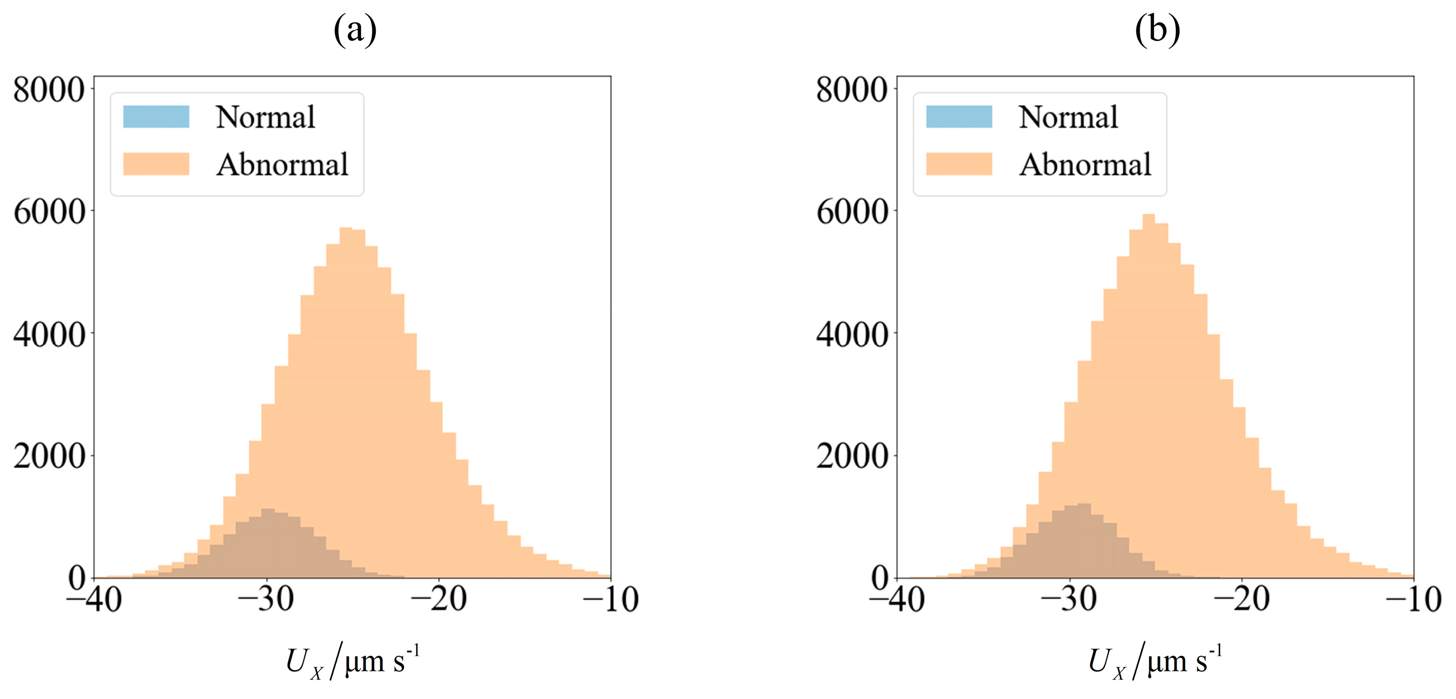
Figure 4.
Velocity of spermatozoa in the test set of 90,000 samples (a) computed using SBT computation and (b) obtained from predictions made using an ensemble of supervised learning trained on 10,000 samples. The blue and orange region represents the number of morphologically normal and abnormal cells, respectively. The sperm cells are subjected to C0 = −1 mN/mm3.

Figure 5.
Sperm in 2D channel heading in the negative X-direction, subjected to magnetic force and a flow in the positive X-direction.
Figure 5.
Sperm in 2D channel heading in the negative X-direction, subjected to magnetic force and a flow in the positive X-direction.

Figure 6.
(a) Cumulative mean flagellum length (red line), head length (green line), and computed velocity (blue line) normalised with respect to mean values obtained from 100,000 samples; (b) proportion of morphologically normal cells in percentage points. The x-axis, in logarithmic scale, of each plot denotes the number of samples used in the computation.

Figure 7.
(a) Sperm subjected to no external field, versus (b) sperm subjected to C0 of −1 mN/mm3. Purity χ computed using 100,000 samples (blue star) for different yield η, compared with purity obtained from supervised learning algorithms trained on 10,000 samples to predict remaining 90,000 samples (hollow red markers) using k-nearest neighbor (circle), ridge regression (square), random forest (triangle) and artificial neural network (inverted triangle).

Figure 8.
Purity as a function of C0. The red circles, green squares and blue triangles denote the computed purity corresponding to a yield of 50%, 70% and 90%, respectively. The dotted lines in matching color are the best-fit polynomials.
Figure 8.
Purity as a function of C0. The red circles, green squares and blue triangles denote the computed purity corresponding to a yield of 50%, 70% and 90%, respectively. The dotted lines in matching color are the best-fit polynomials.
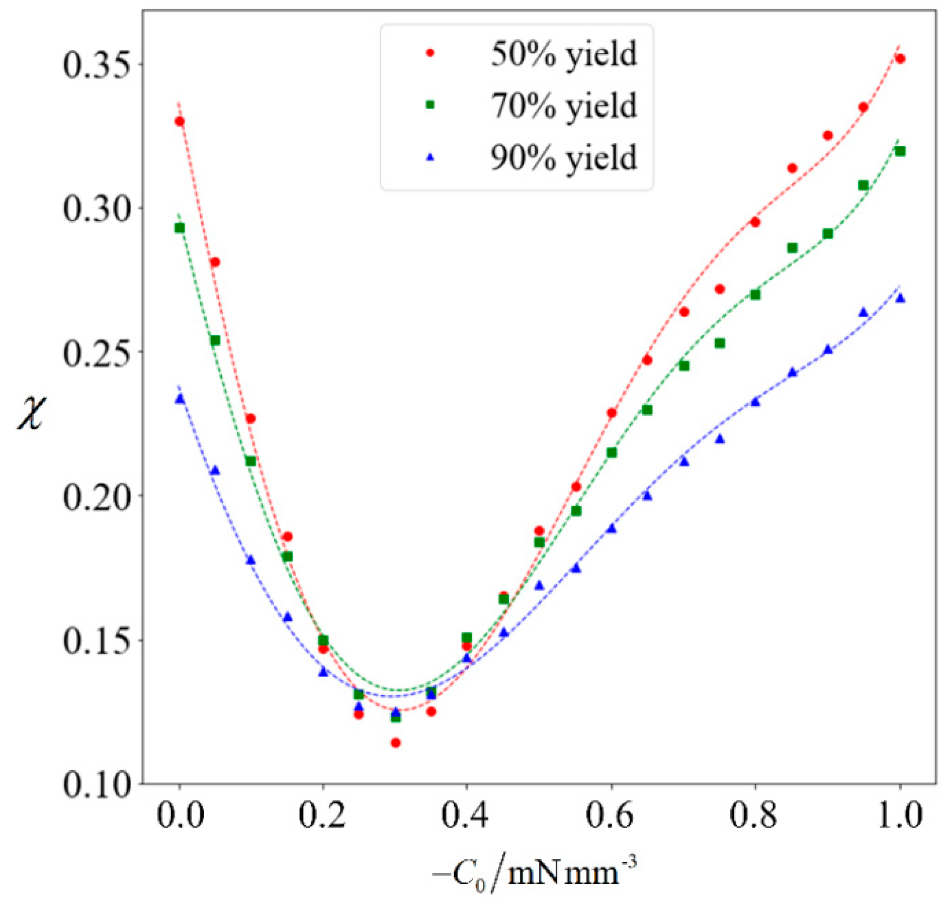
Figure 9.
Flowchart illustrating possible approaches to investigate the non-deterministic process of sperm sorting.
Figure 9.
Flowchart illustrating possible approaches to investigate the non-deterministic process of sperm sorting.
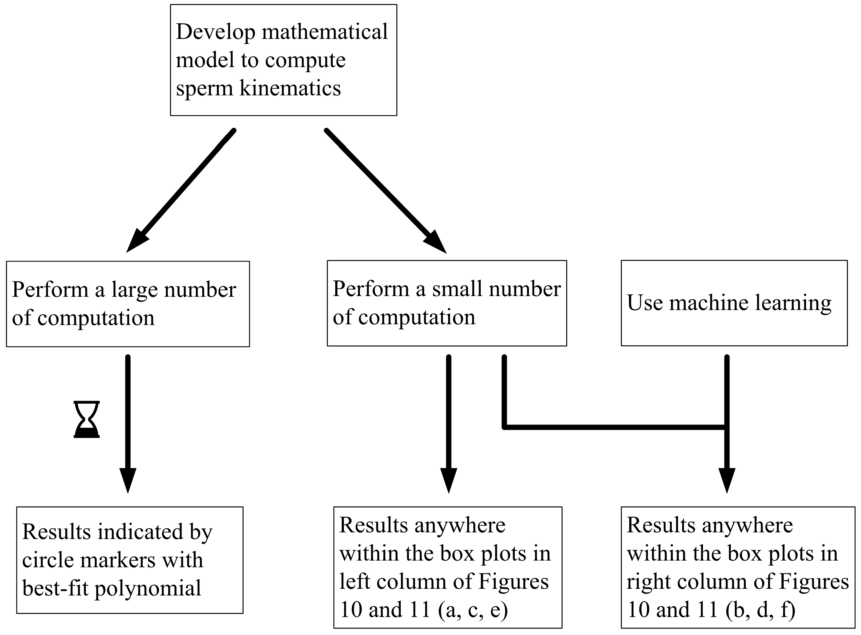
Figure 10.
Boxplots representing results computed (left column) and predicted (right column) from training sets of size 100, 1000, and 10,000 samples in the first row (a,b); second row (c,d) and third row (e,f), respectively. The circle markers are results computed from 105 samples, while the dashed-line is the best fit polynomial. A C0 value of −1 mN/mm3 is used for sorting. The machine learning model makes predictions on the remainder of the 100,000 samples less those used for training.
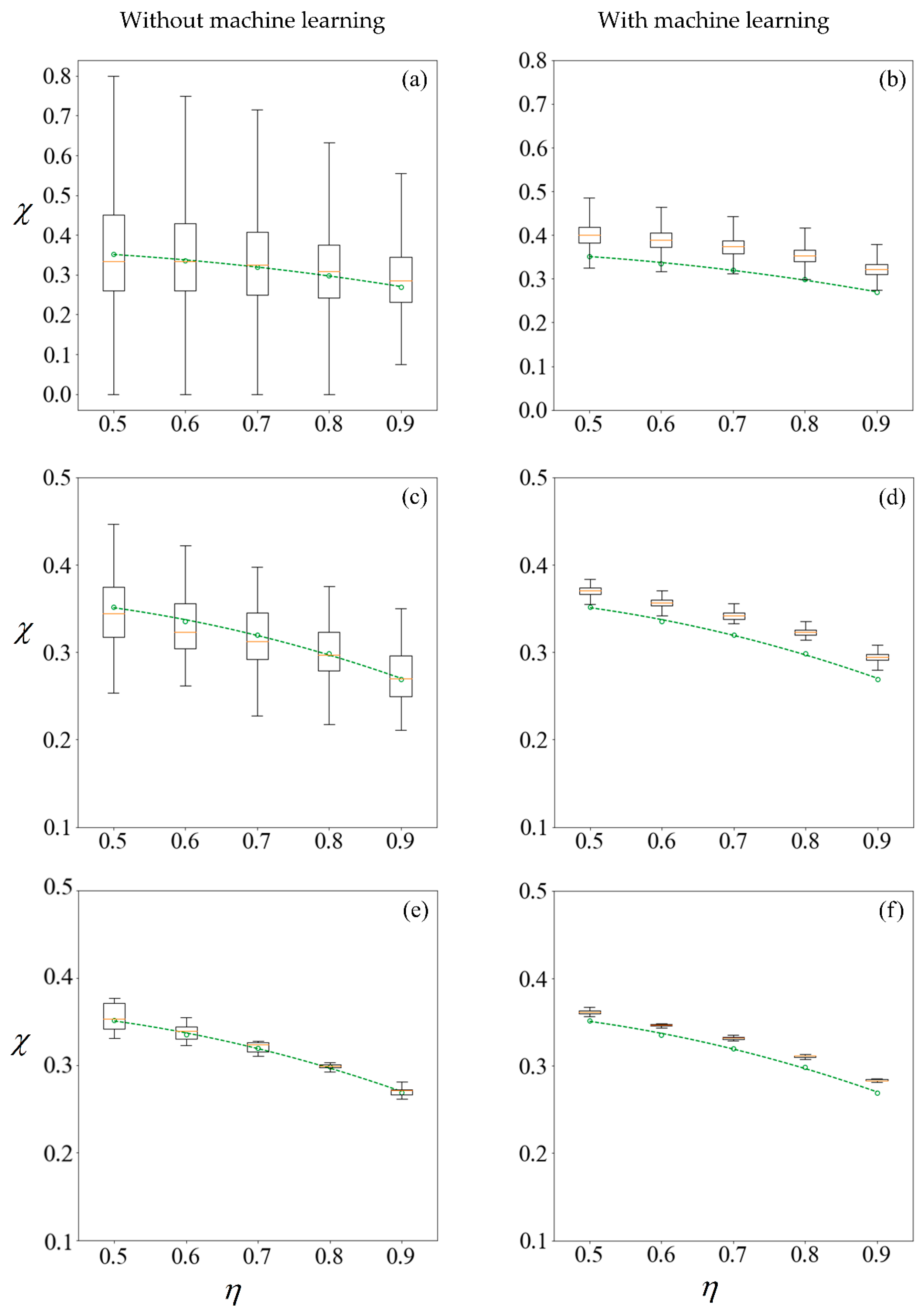
Figure 11.
Boxplots representing results computed (left column) and predicted (right column) from training sets of size 100, 1000, and 10,000 samples in the first row (a,b); second row (c,d) and third row (e,f), respectively. The circle markers are results computed from 105 samples, while the dashed-line is the best fit polynomial. The sperm cells are not subjected to any applied field. The machine learning model makes predictions on the remainder of the 100,000 samples less those used for training.


Table 1.
Categories of sperm according to their head morphology, and the corresponding flagellum beat frequency and amplitude given with their respective standard deviations. Data from [32].
Table 1.
Categories of sperm according to their head morphology, and the corresponding flagellum beat frequency and amplitude given with their respective standard deviations. Data from [32].
| Types of Head | Normal | Amorphous | Elongated Tapering | Piriform Tapering | Megalo-Cephalic |
|---|---|---|---|---|---|
| lh/µm | 3–5 | 3–5 | >5 | 3–5 | >5 |
| wh/µm | 2–3 | >3 | <3 | <2 | >3 |
| f/Hz | 15.2 ± 0.7 | 13.3 ± 1.0 | 13.0 ± 0.9 | 12.2 ± 1.3 | 11.2 ± 1.4 |
| b/µm | 4.76 ± 0.27 | 4.73 ± 0.43 | 4.98 ± 0.33 | 5.36 ± 0.45 | 4.96 ± 0.70 |
© 2018 by the authors. Licensee MDPI, Basel, Switzerland. This article is an open access article distributed under the terms and conditions of the Creative Commons Attribution (CC BY) license (http://creativecommons.org/licenses/by/4.0/).
Share and Cite
MDPI and ACS Style
Koh, J.B.Y.; Shen, X.; Marcos. Supervised Learning to Predict Sperm Sorting by Magnetophoresis. Magnetochemistry 2018, 4, 31. https://doi.org/10.3390/magnetochemistry4030031
AMA Style
Koh JBY, Shen X, Marcos. Supervised Learning to Predict Sperm Sorting by Magnetophoresis. Magnetochemistry. 2018; 4(3):31. https://doi.org/10.3390/magnetochemistry4030031
Chicago/Turabian StyleKoh, James Boon Yong, Xinhui Shen, and Marcos. 2018. "Supervised Learning to Predict Sperm Sorting by Magnetophoresis" Magnetochemistry 4, no. 3: 31. https://doi.org/10.3390/magnetochemistry4030031
Note that from the first issue of 2016, this journal uses article numbers instead of page numbers. See further details here.