The Interaction of Two Surface Vortices Near a Topographic Slope in a Stratified Ocean

Abstract

We study the influence of bottom topography on the interaction of two identical vortices in a two-layer, quasi-geostrophic model. The two vortices have piecewise-uniform potential vorticity and are lying in the upper layer of the model. The topography is a smooth bottom slope. For two cyclones, topography modifies the merger critical distance and the merger efficiency: the topographic wave and vortices can advect the two cyclones along the shelf when they are initially far from it or towards the shelf when they are initially closer to it. They can also advect the two cyclones towards each other and thus favour merger. The cyclones deform, and the potential vorticity field undergoes filamentation. Regimes of partial vortex merger or of vortex splitting are then observed. The interaction of the vorticity poles in the two layers are analysed to explain the evolution of the two upper layer cyclones. For taller topography, two new regimes appear: vortex drift and splitting; and filamentation and asymmetric merger. They are due to the hetonic coupling of lower layer vorticity with the upper layer vortices (a heton is a baroclinic vortex dipole, carrying heat and momentum and propagating horizontally in the fluid), or to the strong shear that the former exerts on the latter. The interaction of two anticyclones shows regimes of co-rotation or merger, but specifically, it leads to the drift of the two vortices away from the slope, via a hetonic coupling with oppositely-signed vorticity in the lower layer. This vorticity originates in the breaking of the topographic wave. The analysis of passive tracer evolution confirms the inshore or offshore drift of the fluid, the formation of tracer fronts along filaments and its stirring in regions of vortex merger. The trajectories of particles indicate how the fluid initially in the vortices is finally partitioned.

1. Motivation of the Study

Vortices are prevalent and long-lived features of ocean dynamics. They play a key role in the transport of momentum, heat, salt, chemical tracers and biological species, across the ocean basins. They can be surface intensified, like the warm-core rings of the Gulf Stream, or thermocline-intensified vortices, like meddies (eddies of Mediterranean outflow water) in the Northeastern Atlantic Ocean [1]. Oceanic vortices can exist both at the mesoscale (with radii comparable to the first internal deformation radius) and at the submesoscale (with smaller radii; [2]). Vortices can be generated at the submesoscale and then merge to grow in size to the mesoscale [3]). The merging process is that by which two like-signed vortices, at the same depth, collapse to form a larger vortex. Vortex merger has been observed in the ocean for Gulf Stream rings [4] and also for meddies [5,6,7].

The process of vortex merger has been studied in simple configurations; the evolution of two equal vortices, or of two unequal vortices, with initially axisymmetric velocities, in the absence of external currents, has been investigated in two-dimensional incompressible flows [8,9,10,11,12,13,14,15,16] and in rotating, stratified flows [17,18,19,20,21,22,23,24,25,26]. In these studies, the two vortices interacted in the absence of bottom topography.

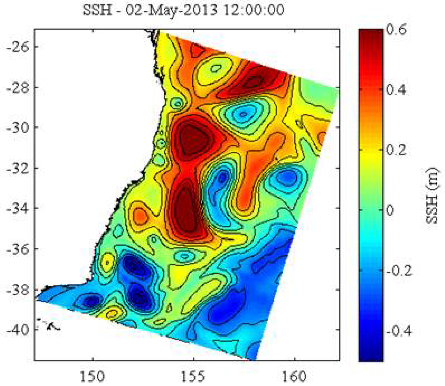
Interactions of like-signed oceanic vortices have also been observed near coasts. Figure 1 shows the interaction of two anticyclones near the east coast of Australia.

In such a case, each vortex not only interacts with its partner, but also with the coastal bathymetry.

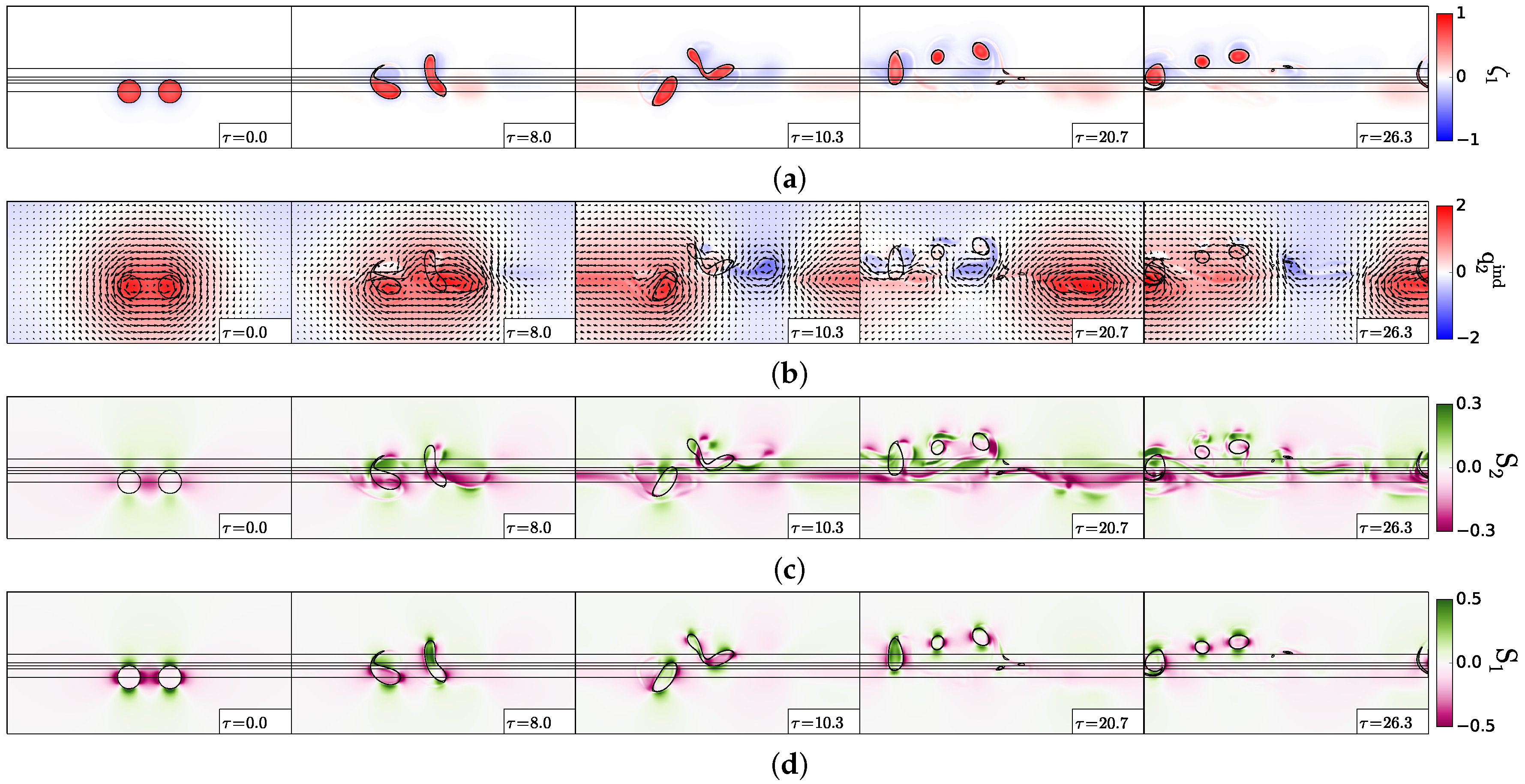
The interaction of a single vortex with a topographic step has already been studied. McDonald [27] showed that cyclones are drawn towards the shallow region (also called “the shelf” hereafter) and that anticyclones are repelled away from it, into the deep region. Indeed, a cyclone (referred to as a “primary cyclone” hereafter) advects fluid from offshore onto the shelf to its right and shelf fluid offshore to its left. The former fluid column is squeezed vertically and develops anticyclonic relative vorticity, while the latter is stretched vertically and becomes cyclonic. These fluid columns, which have acquired vorticity, are called “secondary vortices”. The flow field created by this secondary dipole advects the primary cyclone shoreward (see also Figure 2a of [28]). The opposite effect holds for anticyclones, which are advected offshore by these secondary vortices. Dunn et al. (2001) [29] showed that, for a tall topographic step, vortices can drift with the topographic wave in a steady motion. Zhang et al. (2011) [30] also studied the transport of shelf water, associated with the topographic wave-vortex interaction. They found that the topographic vortex created by a cyclone remains near the shelf, while that created by an anticyclone couples with it and moves offshore; therefore anticyclones are more capable of advecting water away from the shelf. It has been shown that the interaction of ocean vortices with the bottom slope can produce smaller (submesoscale) vortices by forcing and then destabilising a bottom boundary layer [31,32].

Vortex merger near a topographic step in a stratified fluid has however not yet been addressed. This process raises several questions:

(1)

Under which conditions can two surface vortices merge near a topographic step or slope?

(2)

What are the other nonlinear regimes they can undergo and why?

(3)

What are the consequences of these various interactions on the cross-shelf transport?

This problem is complex due to the number of parameters involved (vortex radius, intensity, mutual distance of the vortices, distance to the shelf, topographic slope, height of the shelf, planetary beta effect). Here, we reduce the problem to a simple configuration to render it tractable. We consider two vortices, with piecewise uniform potential vorticity, in a two-layer quasi-geostrophic model on the f-plane. The slope is a hyperbolic tangent in the meridional direction.

The paper is organised as follows: Section 2 presents the methods and models. Section 3 describes the various nonlinear regimes for the interaction of two cyclones. Section 4 analyses these regimes and the influence of topographic height. Section 5 is devoted to the interaction of two anticyclones. Section 6 addresses the evolution of tracer and particles in the flow field and their exchange across the slope. Finally, conclusions are presented in Section 7.

2. The Mathematical Model

2.1. Model Governing Equations

The quasi-geostrophic equations govern the dynamics of stratified flows strongly constrained by planetary rotation (flows with small Froude and Rossby numbers) and with moderate meridional extent. Denoting U the horizontal velocity magnitude, L the horizontal length scale, H the thickness of the flow, N the buoyancy frequency, $f=f_0+\beta y$ the Coriolis parameter in the domain (at any latitude) ($f_0$ being the Coriolis parameter at the centre of the domain, y the meridional distance to this centre, $\beta$ the meridional gradient of the Coriolis parameter), the Froude number is $Fr=U/NH\ll 1$, the Rossby number is $Ro=U/fL\ll 1$ and the meridional extent of the flow, L, is bounded by $L\ll f_0/\beta$.

In a fluid composed of two superimposed layers of uniform (but different) densities, these quasi-geostrophic equations are written:

$${\partial }_t{q}_j+\overrightarrow{u_j}·\overrightarrow{\nabla }{q}_j={\nu }_4{\nabla }^4{\omega }_j$$

(1)

where $j=1,2$ is the upper, lower layer index. The right-hand side of Equation (1) is the biharmonic dissipation of vorticity, implemented numerically to remove vorticity accumulation at small scales, and ${\nu }_4$ is called hyperviscosity. The layer-wise total potential vorticity is:

$$q_j={\nabla }^2{\psi }_j+F_j({\psi }_k-{\psi }_j)+f+{\delta }_{j,2}f{h}_b/H_2$$

(2)

where ${\psi }_j$ is the stream function in layer j. We used $k=3-j$.

Due to the small meridional extent of the domain considered in this study, we keep $f=f_0$ here. The layer coupling coefficients are $F_j=f_0^2/\left(g^{\prime }{H}_j\right)$ with $H_j$ the thickness of layer j and $g^{\prime }=g({\rho }_2-{\rho }_1)/{\rho }_0$ the reduced gravity. ${\rho }_0$ is an average density, and ${\delta }_{i,j}$ is the Kronecker symbol. The internal deformation radius is $R_d=\sqrt{\left(g^{\prime }{H}_1{H}_2\right)/H}/f_0$, and its inverse is called $\gamma =1/R_d$. Here, equal layer thicknesses are chosen $H_1=H_2=0.5,H=1$. The two-layer model is appropriate for surface-intensified flows in the ocean (Flierl, 1978).

The topographic height (from the deepest bottom) is $h_b\left(y\right)$ here (see its mathematical form in Section 2.2; note that the choice of direction for the topographic gradient is arbitrary with respect to the f-plane). The relative vorticity is:

$${\zeta }_j={\partial }_x{v}_j-{\partial }_y{u}_j={\nabla }^2{\psi }_j$$

(3)

the horizontal velocity being:

$$u_j=-{\partial }_y{\psi }_j,v_j={\partial }_x{\psi }_j$$

(4)

From this velocity, we can define the velocity shear in layer j:

$$S_j={\partial }_x{v}_j+{\partial }_y{u}_j$$

(5)

the strain rate in layer j:

$$T_j={\partial }_x{u}_j-{\partial }_y{v}_j$$

(6)

and finally the Okubo–Weiss quantity:

$$O{W}_j=S_j^2+T_j^2-{\zeta }_j^2$$

(7)

It distinguishes regions where deformation is dominant from those of concentrated vorticity.

We remind that the vertical (barotropic and baroclinic) modes are defined by:

$${\psi }_t=(H_1{\psi }_1+H_2{\psi }_2)/H,{\psi }_c={\psi }_1-{\psi }_2$$

(8)

For convenience, we call:

$$q_{dj}={\zeta }_j+F_j({\psi }_k-{\psi }_j)$$

(9)

the potential vorticity anomaly (note that $q_{d1}=q_1$).

We call topographic vorticity the term:

$$q_{topo}=f_0{h}_b/H_2$$

(10)

In our analyses, we use the quantity:

$$q_{2i}={\zeta }_2-F_2{\psi }_2$$

(11)

that we call the “equivalent barotropic” potential vorticity of the lower layer. From this quantity, the lower layer stream function (velocity) can be directly diagnosed (by inverting a Helmholtz operator).

2.2. Numerical Model

Equations (1) and (2) for the quasi-geostrophic model have been implemented numerically in a square, biperiodic domain, using a pseudo-spectral technique in space and a mixed Euler-leapfrog scheme in time. The time step is bounded by the Courant–Friedrich–Levy condition, $\Delta t<\Delta x/U_{max}$. The domain length and width used are $L=4\pi$ (with $x,y\in [-2\pi ,2\pi ]$). Model simulations are performed with 512 collocation points. Very weak biharmonic viscosity is applied in the model (${\nu }_4=5\times {10}^{-8}$). This viscosity does not alter the physical results of the model and only removes small-scale noise.

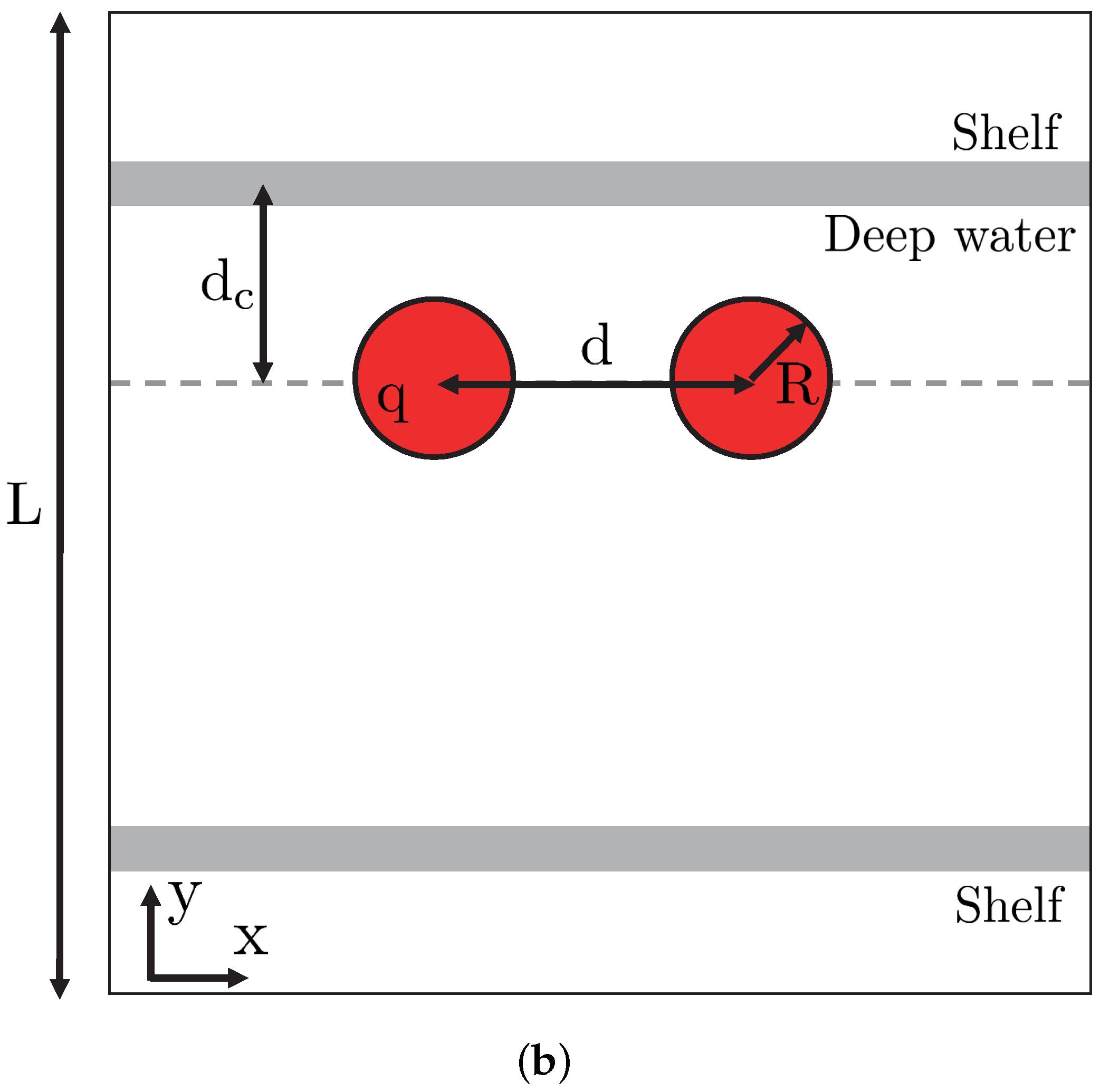
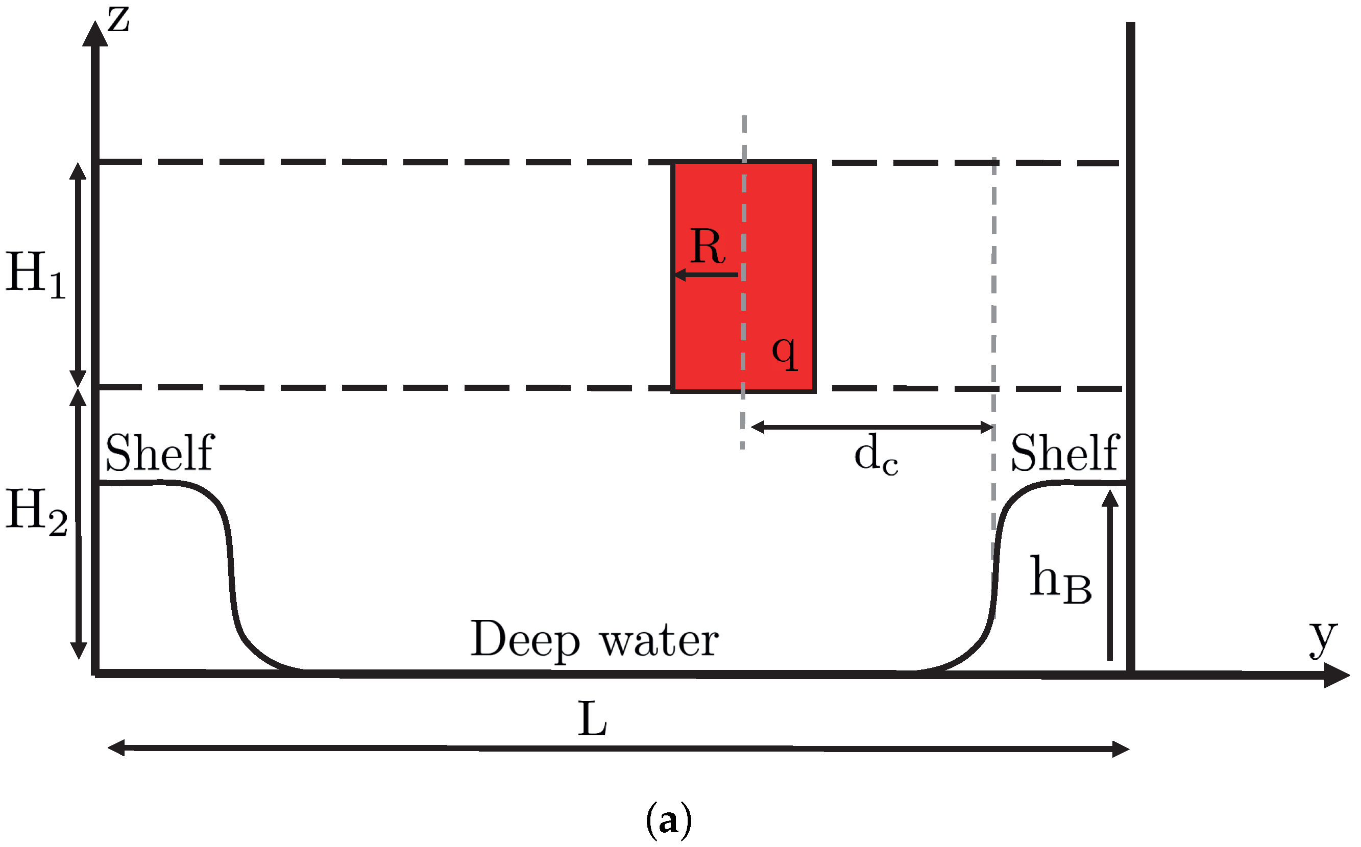
The initial conditions of this model are a pair of identical, circular vortices of radius $R=0.5$, enclosing uniform quasi-geostrophic relative vorticity $q_1=1$ (when we investigate the interaction of two cyclones) or $q_1=-1$ (when we study the interaction of two anticyclones), lying at a distance d from each other and at a distance $d_c$ from the topography. Elsewhere, $q_1=q_{d2}=0$ (see Figure 2).

As an application to the ocean, the East Australian eddies have a peak velocity $V\sim 0.5m/s$ at a radius $R\sim 50$ km. Using an estimate of vorticity $q\sim 2\zeta \sim 4V/R=4\times {10}^{-5}$ s${}^{-1}$, length and time are scaled between the model and the ocean via $L_s={10}^{5}m$ and $T_s=2.5\times {10}^{4}s$. At 35 ${}^{\circ }$S, $f_0=8.34\times {10}^{-5}{s}^{-1}$, so that $q/f_0=0.5$ (note that $Ro=0.12$). The radius of deformation is about 50 km so that the Burger number $Bu\sim 1$. The relative influence of the beta-effect is weak, since the vortices are mesoscale features; here, $\beta L/f_0\sim 1.2{10}^{-2}$, and the vortex radius is small compared with the Rhines scale $L_{Rh}=\sqrt{V/\beta }$, a scale above which the beta effect is influential on the dynamics. Here, $L_{Rh}\sim 160$ km.

In the model, the dimensionless value of $f_0$ is therefore $2.0$, which scales the topographic vorticity $f_0{h}_b/H_2$ in Equation (3). The maximal value of $h_{b0}/H_2$, used in this study is $0.3$. Note that the quasi-geostrophic model assumptions are met since the Rossby number is small, the Burger number is unity, the beta effect is weak and the topographic amplitude remains moderate.

Nevertheless, this validity is limited to mesoscale vortices, near low shelves, at mid-latitudes. The interaction between smaller vortices, near taller shelves, should be investigated in a primitive equation model.

The bathymetry is a smooth slope both north and south (for positive and negative y’s):

$$h_b\left(y\right)=h_{b0}[1.0+0.5\tanh ((y-y_t)/L_t)-0.5\tanh ((y+y_t)/L_t)]$$

(12)

The topographic gradient thus defines the meridional direction. The choice of parameter values for cyclonic solutions is $y_t=3,L_t=0.25$ and $y_t=5,L_t=0.25$ for anticyclones. The shallow region is wider in the former case, because cyclones tend to climb on topographic slopes; therefore, a significant part of their evolution is expected to take place in the shallow region (the “shelf”), if they are not too far away from it initially. Due to meridional periodicity of the domain (the isobaths giving the zonal direction), the shelf forms a single region.

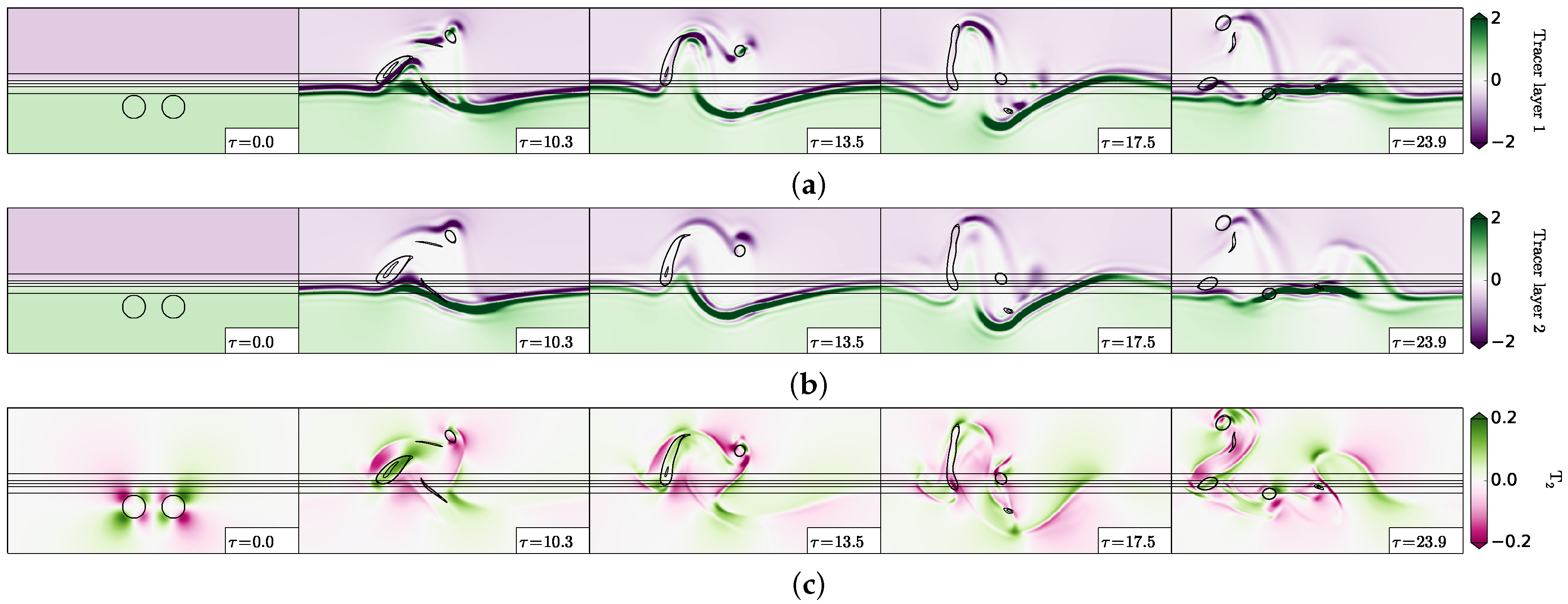
To track fluid masses, a passive tracer, with initial distribution equal to one over the shelf and to minus one in the deep region, is used to study the evolution of shallow and deep fluid masses. Note that the passive scalar field has the same resolution and undergoes the same dissipation as vorticity.

Furthermore, 10,000 particles were seeded in the flow (over the shelf, in the deep region and in the vortices). Their advection (via a Euler scheme) and tracking allow us to follow the fluid from the vortex cores.

3. Interaction of Two Cyclones: Nonlinear Regimes

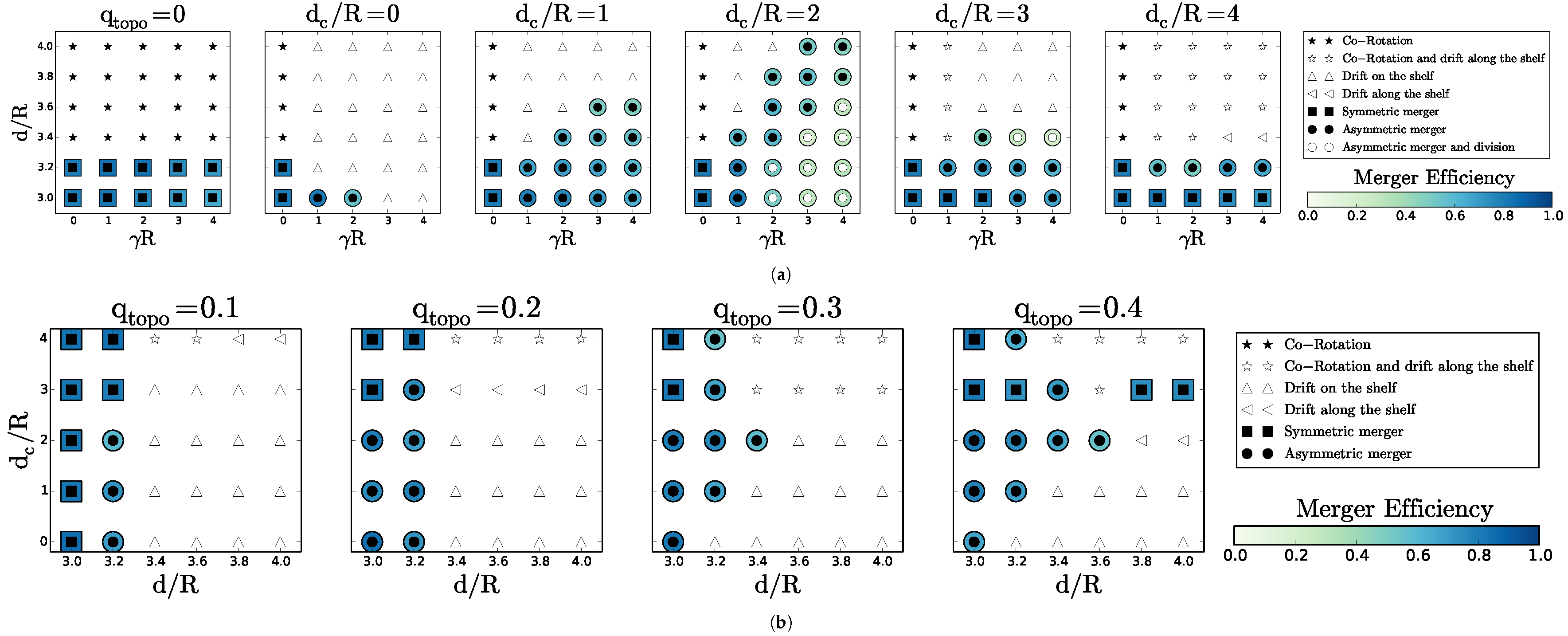
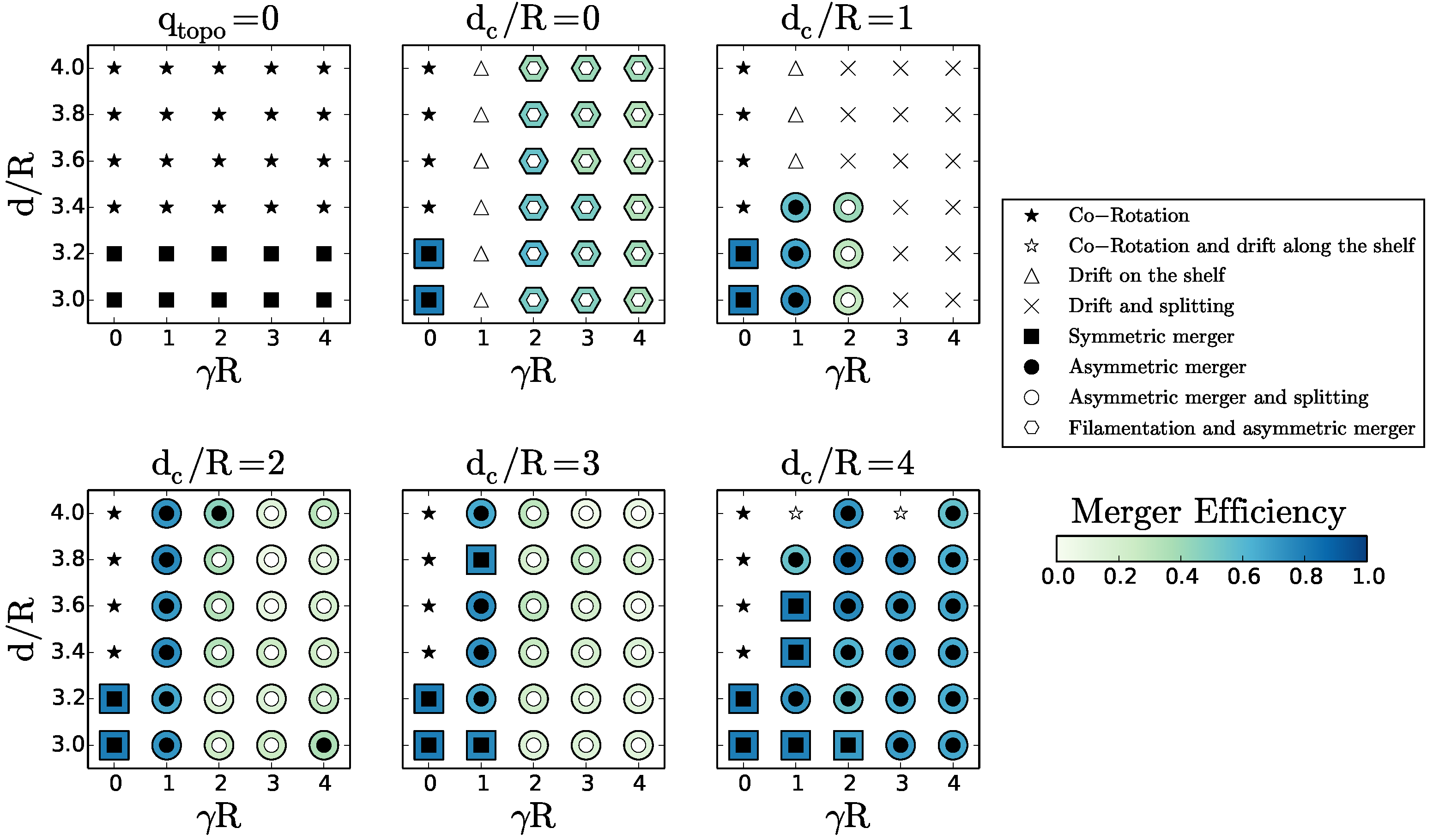
Three hundred numerical simulations have been performed varying the non- dimensional distance between the two cyclones $d/R$, their distance to the slope $d_c/R$, the rescaled density stratification $\gamma R$ and the topographic vorticity $f_0{h}_{b0}/H_2$. Figure 3 summarises the main regimes in the parameter space.

The left-hand panel in Figure 3a is similar to the results obtained by Polvani (1989) [33], for vortex merger over a flat bottom in a two-layer quasi-geostrophic model: in this case, merger occurs for $d/R<3.3$. The invariance of the nondimensional critical merger distance $d^{*}=d/R$ with respect to stratification in this study is related to the vortex initialisation as a disk of constant potential vorticity. When vortices are initially disks of uniform relative vorticity, the critical merger distance depends on stratification via hetonic effects [18,19,34,35,36,37]. Indeed, relative vorticity in one layer induces interface deviation between layers and thus potential vorticity of opposite sign in the other layer. This in turn can lead to vertical coupling of these vorticity poles and to their self-advection, counter-acting the merging process.

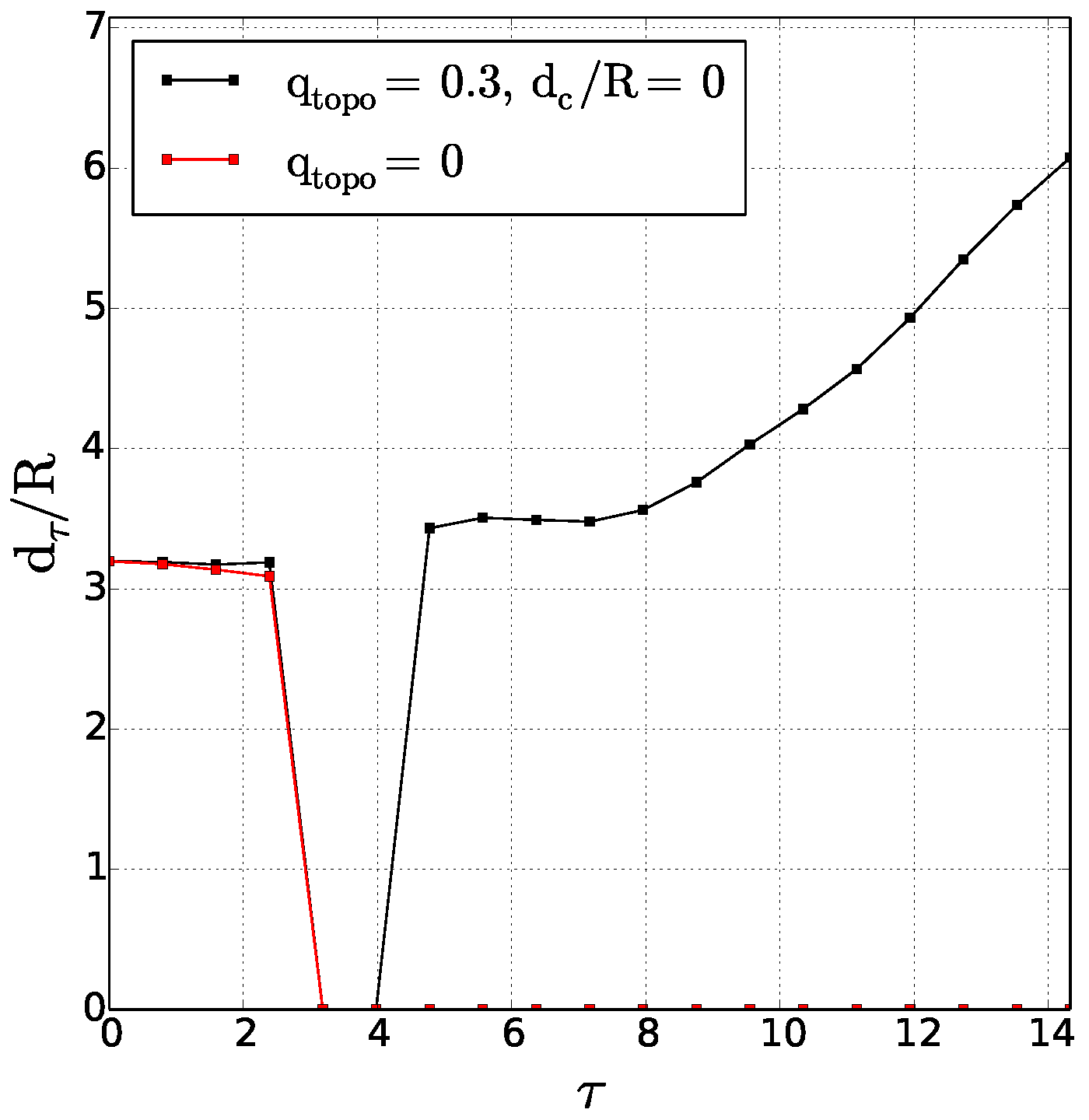
In the presence of topography, the two cyclone evolution is similar to that over a flat bottom, if they lie far away from the slope. Merger occurs again for $d^{*}=3.3$; the weak influence of topographic waves leads to asymmetric merger. If the two cyclones are initially more distant from each other than $d^{*}$, co-rotation and drift along the slope are the main evolutions. Note that, in the large $d_c/R$ limit, the co-rotating cyclone pair can drift steadily along the topography.

An analytical solution for a point vortex doublet drifting steadily along a step-like shelf can be obtained, with approximations (see Appendix A). This solution shows that (1) stationary drift of a vortex doublet is possible far away from the shelf and (2) this doublet induces a wave in topographic vorticity, which displaces the doublet.

If the vortex pair is initially close to the slope, new regimes appear:

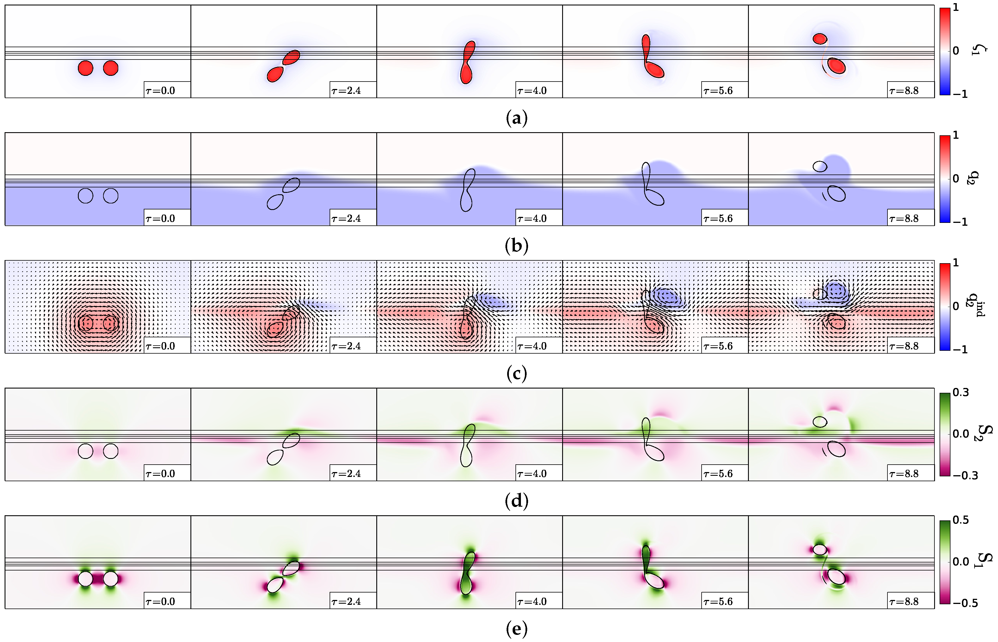
(i)

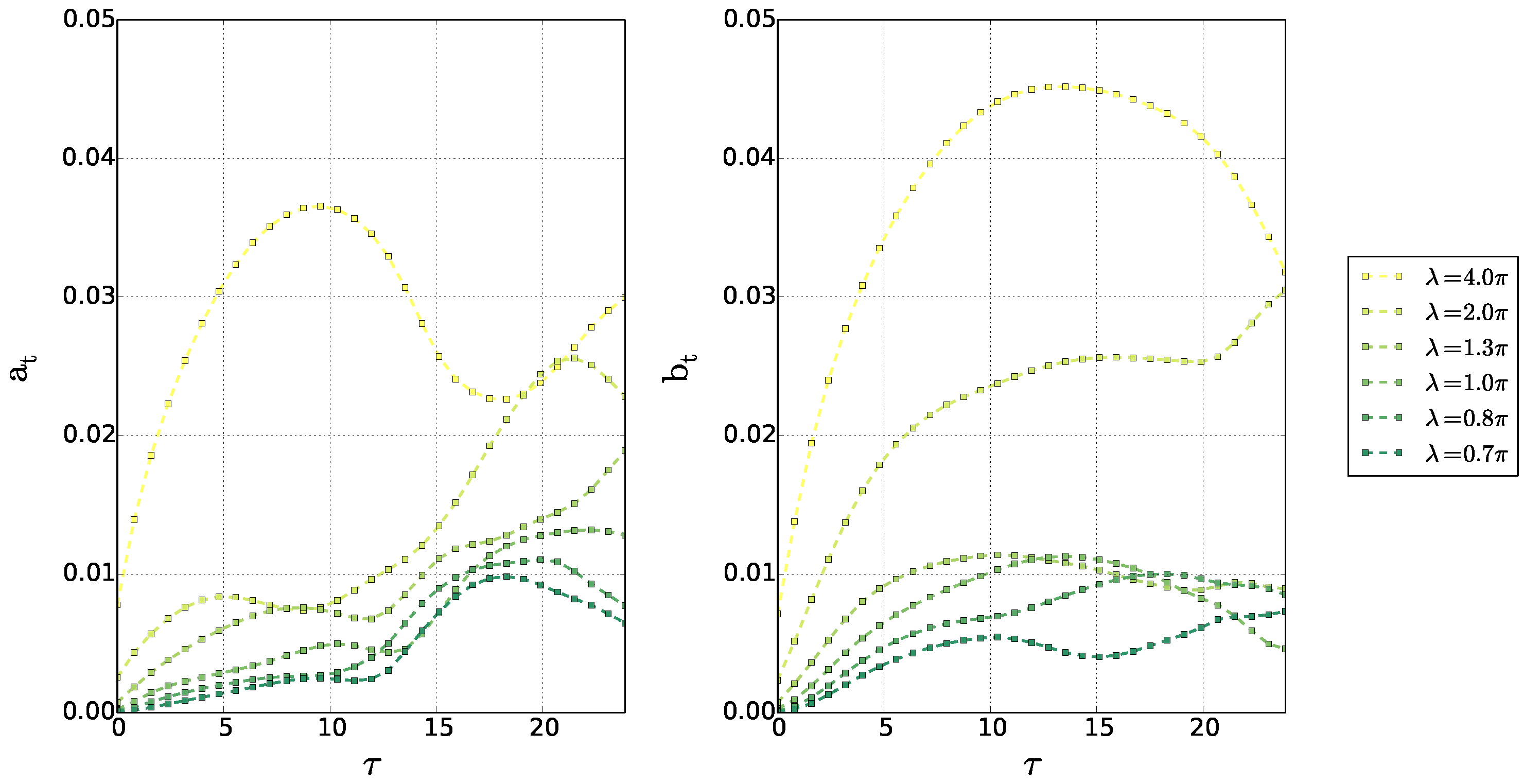
Asymmetric, partial merger can occur as negative potential vorticity in the lower layer creates a flow in the upper layer; this flow advects one cyclone towards the other; then, the two cyclones merge. Thus, merger occurs for two cyclones initially more distant than $3.3R$. However, the lower layer vorticity poles exert a shear on the upper layer cyclones, which filament. Therefore, the efficiency of the merging process is reduced. We define merger efficiency as the ratio of the final (merged) vortex area integral of potential vorticity (in Layer 1), to that of the two initial vortices:

$$ME=\frac{\int \int q_{final}dS}{\int \int q_{initial}dS}$$

(the area is bounded by the outermost closed vorticity contour). This efficiency is maximal for the evolution called complete vortex merger, during which nearly all the fluid contained in the two initial vortices (and the potential vorticity of these fluid particles, which is a Lagrangian invariant) goes into the final, merged, vortex. Indeed, during this evolution, only a small percentage of the initial vortex fluid (usually less than 5%) is finally contained in the peripheral filaments, which ensure angular momentum conservation.

Figure 3 shows that asymmetric merger is less efficient than symmetric merger.

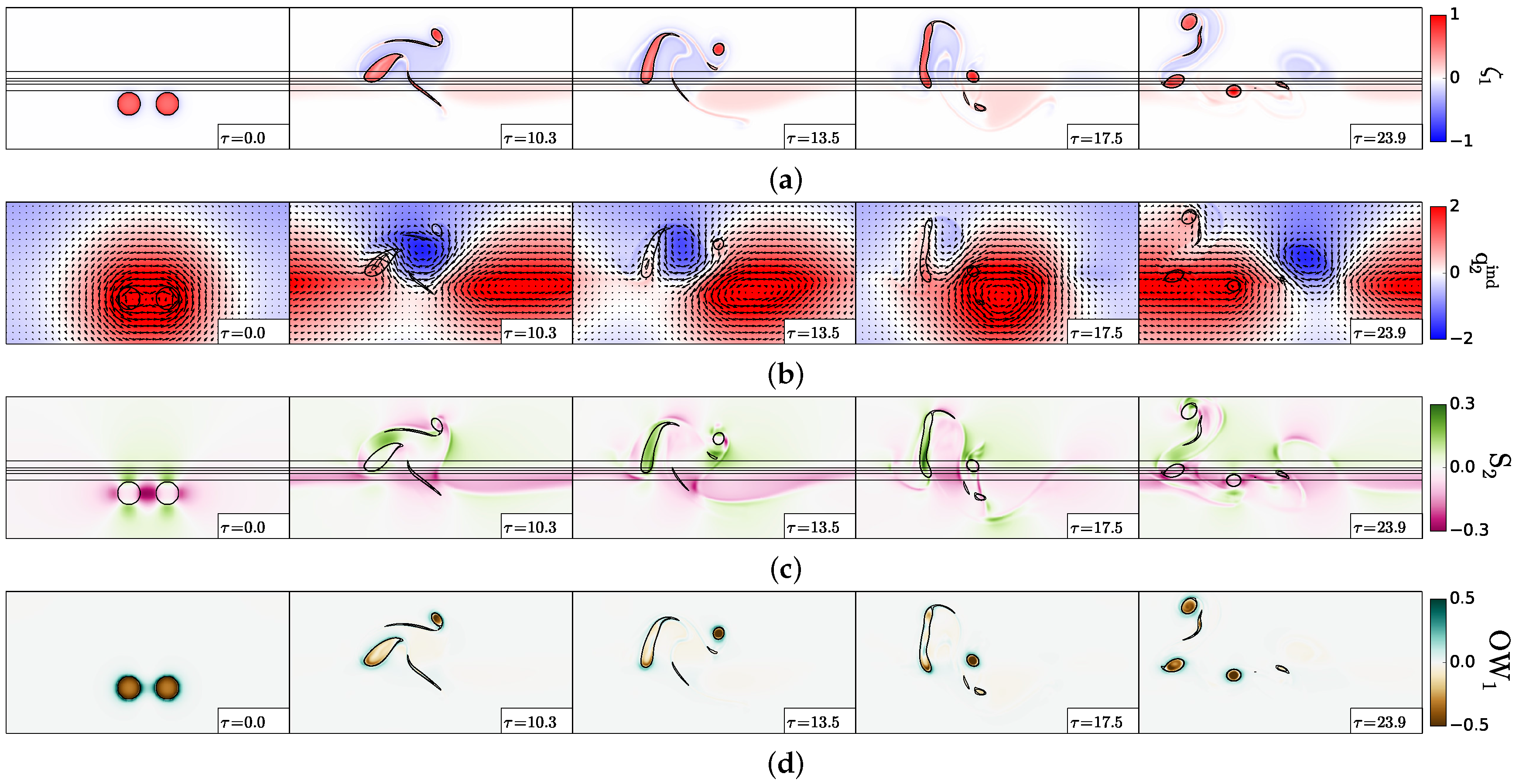
(ii)

Asymmetric merger and splitting: The vortex resulting from merger is elongated and subject to intense shear from its cyclonic partner and from topographic vortices (topographic vortices are formed by the amplification, steepening and breaking of topographic waves); this merged vortex splits into two parts. This evolution can occur when $\gamma R$ is large enough to couple the motions vertically. In this case, the merger efficiency is very small.

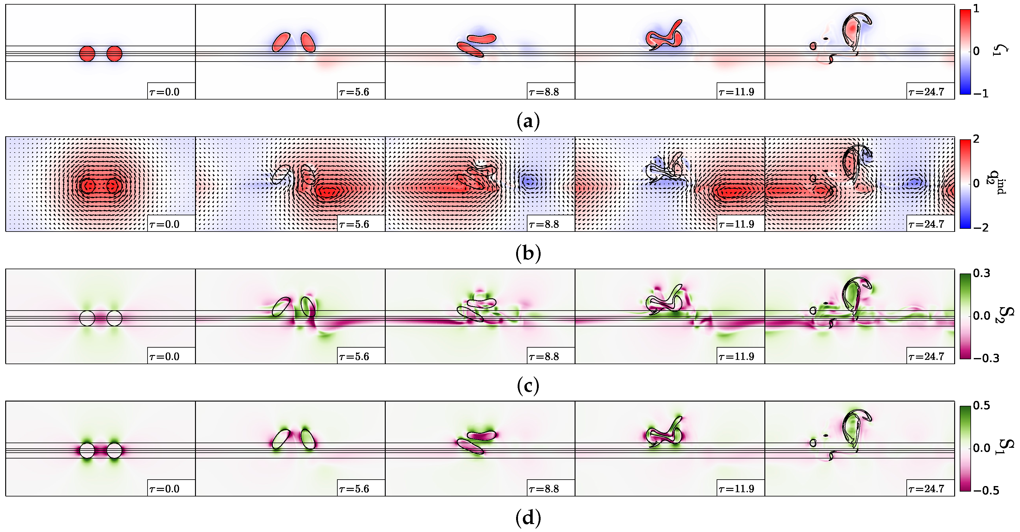
(iii)

Drift towards the slope and on the shelf: when the vortices are close enough to the slope, the topographic wave and subsequently formed vortices (in the lower layer) can advect both upper layer vortices upon the shelf. Again, this requires sufficient layer coupling (i.e., large values of $\gamma R$).

Figure 3b describes the regimes in the $d/R,d_c/R$ plane for various values of topographic vorticity $q_{topo}$. For small values of $q_{topo}$, the regime diagram shows that the critical merger distance is $d^{*}=3.3$, as for a flat bottom, but the vortex pair is influenced by the topographic waves and can climb on the shelf if $d/R>3.3$.

As the topographic height increases, two main effects are noticed:

(a)

The efficiency of the merger of the two cyclonic vortices is reduced by filamentation, and the merger is only partial.

(b)

Merger occurs for initially more distant cyclones; this is related to the advection of one cyclone towards the other by topographic vortices.

We summarise our results in Figure 4 by plotting the normalised critical merger distance $d^{*}$ against the stratification $\gamma R$, for the various values of the distance of the vortex pair to the topographic slope $d_c/R$.

This figure confirms that far from the slope, the critical merger distance is similar to that over a flat bottom. When the vortices are initially very close to the slope, this critical distance is reduced (the vortices are pushed apart by the topographic wave). For intermediate distances from the slope ($d_c/R\in [1,2]$), the topographic vortices advect the two vortices towards each other and favour merger. This effect is all the stronger as layer coupling (stratification) is strong.

4. Analysis of Main Regimes for the Two Cyclone Interaction

Here, the topographic vorticity is $f_0{h}_{b0}/H=0.3$. We analyse in detail selected examples, the three regimes of interaction specific to the case with bottom topography, which are not observed over a flat bottom, for two equal vortices.

4.1. Partial Merger

Firstly, we analyse the case of a partial merger ($d/R=3.4,\gamma R=1,d_c/R=2$); we present the vorticity and velocity shear fields, in each layer, in Figure 5.

Figure 5a shows the vortices in the upper layer (in relative vorticity distribution). Initially, the two vortices start co-rotating; the easternmost vortex climbs on the slope; it is elongated and starts to merge with its companion vortex. However, finally, the cyclone above the shelf drifts away from its partner in the deep region. This indicates that the topographic effects are stronger than the mutual vortex interaction. This topographic effect is due to the lower layer flow across the topography and to its coupling to the upper layer. Indeed, it can be seen that a perturbation of the interface with large zonal scale grows first in the lower layer (as predicted by Appendix A), but then, as the evolution is unsteady, this wave grows, changes form and couples with the upper layer vortex on the shelf. To assess this coupling, the vorticity and velocity shear distributions in the lower layer are next examined.

Figure 5b shows the total, deep, potential vorticity. It only comprises topographic vorticity initially. This vorticity is advected on the slope by the upper layer cyclonic motion, via vortex stretching. To better identify the effects of this deep vorticity advection, we plot, in Figure 5c, the lower layer “equivalent barotropic” potential vorticity, to which the deep motion is directly related (the deep vorticity field is indicated). In this deep “equivalent barotropic” potential vorticity, one can easily identify the topographic wave, which develops along the slope, with a positive vorticity pole (to the west) and a negative one (to the east). These vorticity poles match the difference in total deep potential vorticity, between the instantaneous and initial values along the slope. A negative vorticity pole grows below and east of the upper layer cyclone on the slope. This deep anticyclone is responsible for (a) the elongation of the upper layer cyclone on the slope (via the shear exerted on it) and (b) the drift of this cyclone towards the shelf (via the hetonic coupling).

Finally, we also compute the velocity shear generated by these deep vorticity poles (Figure 5d); at $\tau =4.0$ and $\tau =5.6$ ($\tau$ is the normalised time, equal to the model time divided by the eddy time scale; the latter is chosen as $T=4\pi /q_{1max}=4\pi$), intense shear is created exactly below the upper layer cyclone on the slope. This lower layer shear is felt in the upper layer via the density interface. Figure 5e indicates how strong the upper layer shear is, in the vortex on the slope, at $\tau =4.0$ and $\tau =5.6$.

Since the deep flow and potential vorticity play a key role in coupling the upper layer vortices and the topography, some further analysis is devoted to their time evolution. In particular, we write the lower layer potential “equivalent barotropic” vorticity equation as:

$${\partial }_t{q}_{2i}=-J({\psi }_2,q_{2i})-F_2{\partial }_t{\psi }_1-J({\psi }_2,F_2{\psi }_1)-J({\psi }_2,f_0{h}_b/H_2)$$

(13)

neglecting dissipation. Here, $J(f,g)={\partial }_{x}f{\partial }_{y}g-{\partial }_{x}g{\partial }_{y}f$ is the Jacobian operator.

This equation states that the lower layer “equivalent barotropic” potential vorticity (that related directly to the deep flow) varies owing to its advection by this deep flow, to the rate of change of the upper layer flow (via layer coupling), to the baroclinic advection of the barotropic flow and to the interaction of the lower layer flow with the topography.

Indeed, the third term in the right-hand side, $-F_{2}J({\psi }_2,{\psi }_1)$ can also be written $F_{2}J({\psi }_c,{\psi }_t)$. This term also represents the barotropic advection of interface deviation. These three components are presented below (Figure 6).

In Figure 6a, the first term in the equation, the advection of lower layer “equivalent barotropic” potential vorticity, is northward, as indicated by the dipole at the middle of the domain.

The second term, the rate of change of the upper layer flow (multiplied by the layer coupling coefficient), is initially related to the rotation of the upper layer vortex pair (see Figure 6b). At later times, it becomes zonally dipolar, corresponding to the meridional advection of one upper layer cyclone to the north. This dipolar structure is related to the growth of a dipole in $q_{2i}$ (see Figure 5c at $\tau =4$ and $\tau =5.6$). This rate of change is twice as strong as the first term. The third term (barotropic advection of interface deviation) is also related to the rotation of the two vortices initially, but then becomes predominant in the northern cyclone for which the northward motion and the velocity shear become strong (see Figure 6c). This term is weaker than the second term. Finally, the last term represents the topographic wave (see Figure 6d). It is concentrated along the slope. It is of the same order as the first and third terms. In summary, though the third term is larger than the other terms, all terms contribute to the upper layer cyclones’ motion and deformation, to the deformation of the lower layer potential vorticity and to the growth of the topographic wave.

The distance between the geometric centres of the upper layer cyclones (see Figure 7) decreases sharply at early times in the presence of the topographic slope, whereas it would remain constant over a flat bottom. After they have joined, the two cyclones diverge spatially; this corresponds to the rapid growth of this distance with time.

4.2. Merger and Splitting

Secondly, we analyse a case of merger and splitting ($d/R=3.4,\gamma R=3,d_c/R=2$); we present the vorticity and velocity shear, in the two layers, in Figure 8. Figure 8a shows that the upper layer vortices merge asymmetrically (between $\tau =0$ and $\tau =10.3$). Then, the merged vortex becomes more elongated (see $\tau =13.5$ and $\tau =17.5$), before splitting into two vortices of nearly equal sizes ($\tau =23.9$). The lower layer “equivalent barotropic” potential vorticity shows a negative pole on the slope, between two positive poles, east and west (see Figure 8b; $\tau =10.3$). A strong shear flow appears between these poles, in particular at the location of the merged vortex. This vortex elongates around this negative pole of $q_{2i}$ and breaks. In the lower layer, the velocity shear is initially the strongest in the periphery of the vortices (see Figure 8c; $\tau =0$). As the merged vortex elongates, this shear reaches its positive maximum inside this vortex (at $\tau =13.5$ and $\tau =17.5$). After splitting, the shear is intense between the vortices.

This deformation is reflected in the upper layer Okubo–Weiss quantity (see Figure 8d). Initially, the two vortex cores are the loci of vorticity concentration, while the shear and strain rates are stronger on their rim. At later times ($\tau =13.5$ and $\tau =17.5$), the deformation rate is not negligible, compared with vorticity, in the merged vortex core. A qualitative model for upper layer vortex splitting is presented in Appendix B. In the two-layer quasi-geostrophic framework, it is possible to estimate the shear created in the upper layer by a lower layer (topographic) vortex and to compare this shear with that necessary to break an upper layer vortex. It occurs that here, the shear is strong enough to induce this splitting. Once split, the two upper layer cyclones are again a region of vorticity concentration.

The distance between the vortices (see Figure 9) decreases sharply with time and vanishes, in the presence of topography; this corresponds to the merging process. Note that the time series is stopped before splitting occurs. Over a flat bottom, merger does not occur, and the distance between vortices does not substantially vary with time.

4.3. Drift towards the Shelf

Finally, we study a case where two cyclones, initially close to each other, drift apart on the shelf ($d/R=3.2,\gamma R=1,d_c/R=0$); we present the vorticity and velocity shear, in the two layers, in Figure 10.

Figure 10a indicates that the two cyclones, initially located on the topographic slope, join at their mid-point, but only briefly ($\tau =2.4$). Soon, they drift apart, being connected only by a filament ($\tau =4.8$). This filament is rapidly dissipated, and the two cyclones become progressively more distant from each other, one remaining on the slope, the other moving northward onto the shelf ($\tau =5.6$ and $\tau =11.9$).

The explanation for this evolution lies in the lower layer (see Figure 10b): the anticlockwise motion of the upper layer vortex pair drives the deep fluid upslope, to its east and downslope to its west. The fluid moving upslope acquires the negative potential vorticity anomaly (to compensate the vertical squeezing of the fluid columns). This negative vorticity tongue couples with both upper cyclones, but as it extends northward, it pairs more efficiently with the northern cyclone. This is confirmed by the structure of the lower layer “equivalent barotropic” potential vorticity (Figure 10c), whose negative pole amplifies north of the slope, east of the two cyclones, and then drifts northeastward with the northern cyclone.

These lower layer potential vorticity poles result from the amplification of the vorticity front deviation; this deviation encompasses two terms, one due to lower layer (topographic) vortices and one due to topographic waves. Note that, at early times, there are no topographic vortices. This deviation is analysed via a Fourier transform of the difference in potential vorticity between any given time and the initial state. This Fourier analysis is performed in the lower layer, over the topographic slope:

$$q_2^{\prime }(x,y,t)=q_2(x,y,t)-q_2(x,y,0)=\sum _{n=0}^N{A}_n(y,t)cos(2n\pi x/L)+B_n(y,t)sin(2n\pi x/L)$$

(14)

for $y_t-L_t<y<y_t+L_t$, and:

$$a_n\left(t\right)=\frac{1}{2L_t}{\int }_{y_t-L_t}^{y_t+L_t}{A}_n(y,t)dy,b_n\left(t\right)=\frac{1}{2L_t}{\int }_{y_t-L_t}^{y_t+L_t}{B}_n(y,t)dy$$

(15)

The time series of $a_n$ and $b_n$ are shown in Figure 11: at early time, the longest wave grows, forced by the vortex pair. This can be seen in the early maps of lower layer potential vorticity. Then, harmonics (shorter waves) develop, as the upper layer vortices come nearer to the slope and as nonlinear interactions transfer energy from one wave to another. Among these harmonics, the first and second are dominant. These harmonics are due to the steepening and finally to the breaking of the topographic wave, which produces a topographic vortex. The higher harmonics have an amplitude comparable to that of the initial wave, when breaking occurs. The wavelength of the second harmonic is nearly equal to the horizontal extent of the vortex pair. Note that, once formed, the topographic vortices not only couple with upper layer vortices and advect them away, but they also deform them.

The time evolution of the distance between the two vortices (Figure 12) shows indeed that the two vortices touch each other, but then drift apart. This separation and drift is due to the presence of the topographic vortices in the lower layer; they create the hetonic effect, which propels the two vortices apart from each other. Indeed, over a flat bottom, the two vortices touch, and merge irreversibly. It can be noticed that (a) there is little difference between the two initial evolutions (over a flat bottom and over the shelf) in terms of vortex separation; but (b) when topography is present, the vortices are finally much more distant than they were initially. The hetonic effect has prevailed over the merging tendency due to the closeness of the vortex pair with the shelf (merging did not have time to occur before the topographic effects set in).

4.4. Influence of Topographic Height

The regime diagram is shown for $f_0{h}_{b0}/H_2=0.6$ in Figure 13. Compared with that for $f_0{h}_{b0}/H_2=0.3$ (Figure 3), asymmetric merger is favoured, both when the two cyclones lie above the slope, or far away from it. Two new regimes appear: vortex drift and splitting, filamentation and asymmetric merger. We describe them hereafter. Note also that by increasing the topographic height, the topographic slope is increased, which favours the growth of topographic waves and of topographic vortices.

4.4.1. Vortex Drift and Splitting

For $d/R=3.6,\gamma R=2.0,d_c/R=1.0$, the two upper layer cyclones drift towards the shelf (see Figure 14a); the easternmost vortex splits above the slope. Finally, three main vortex fragments drift along the slope. This evolution is due to the influence of the lower layer vorticity (Figure 14b). As the upper layer vortices move across the slope, a topographic wave is formed in the lower layer (see, for instance, $\tau =10.3$). At this moment, the easternmost upper vortex is located above and between two lower potential vorticity poles of opposite polarities. These two poles create an intense shear on the upper vortex, which breaks (see again Appendix B for a description and qualitative estimation of this effect). The lower and upper layer shears (Figure 14c,d) indicate a strong shear associated with the topographic wave and also a strong shear on the vortex, which breaks (at $\tau =10.3$).

4.4.2. Filamentation and Asymmetric Merger

The second “new” regime, which appears for taller topographies, is filamentation and asymmetric merger. It is obtained for the same vortex parameters as in the previous case ($d/R=3.6,\gamma R=2.0$), but for vortices initially closer to the topography $d_c/R=0$. This regime is shown in Figure 15.

Initially, the two vortices head towards each other and towards the shelf (see Panel (a) of this figure). Then, they are strongly elongated; they filament, but the tangle of filaments and small eddies finally merges to form one large vortex and peripheral debris.

Again, the explanation of this behaviour is given by the structure of the lower layer “equivalent barotropic” potential vorticity, composed of an alternation of opposite-signed poles (see Panel (b) of the figure). The upper vortices lie above and between these poles (at $\tau =5.6$). The shear is thus strong, and vortex splitting is also favoured by hetonic coupling. This is confirmed by the structure of the shear in both layers (in particular in the lower layer at $\tau =5.6$ and in the upper layer at $\tau =8.8$. Merger occurs only when the filaments and vortices are located above a negative lower layer vorticity pole ($\tau =11.9$).

Finally, the merged vortex is again located above and between a cyclone and an anticyclone of the lower layer and is strongly elongated.

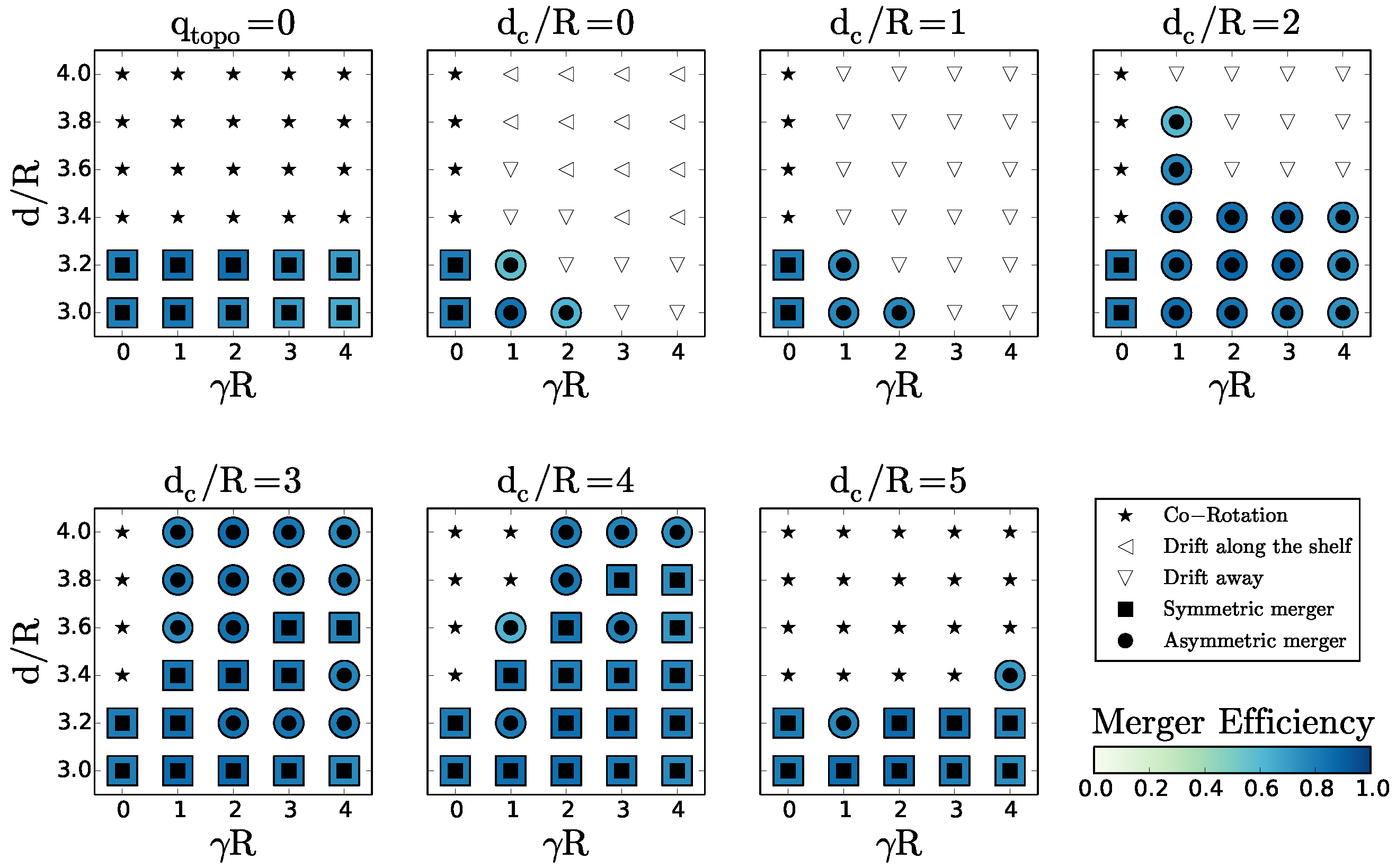
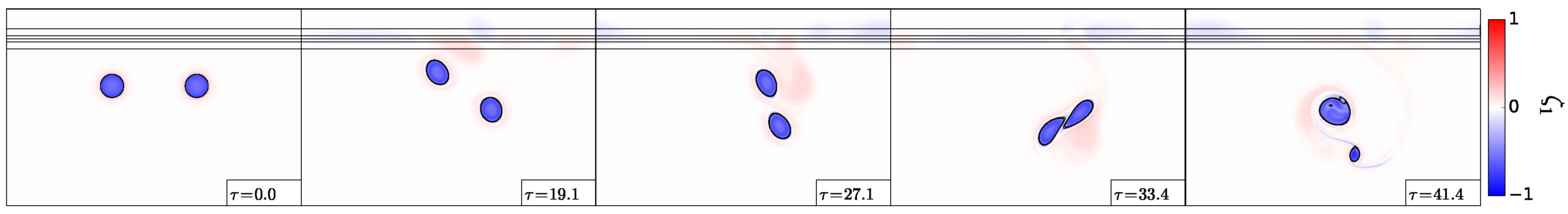
5. Interaction of Two Anticyclones

Previous studies have shown that a single anticyclone tends to drift away from a continental shelf. Thus, it is expected that the interaction of two anticyclones will be accompanied by such a drift.

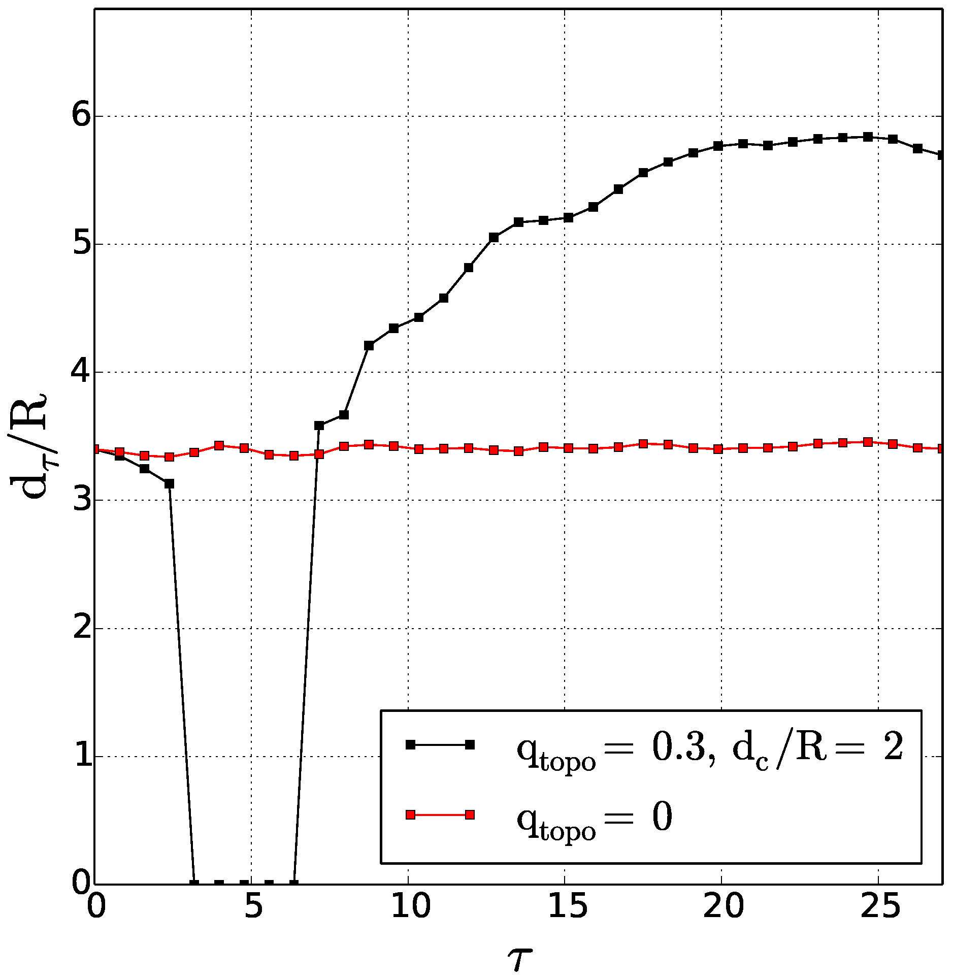
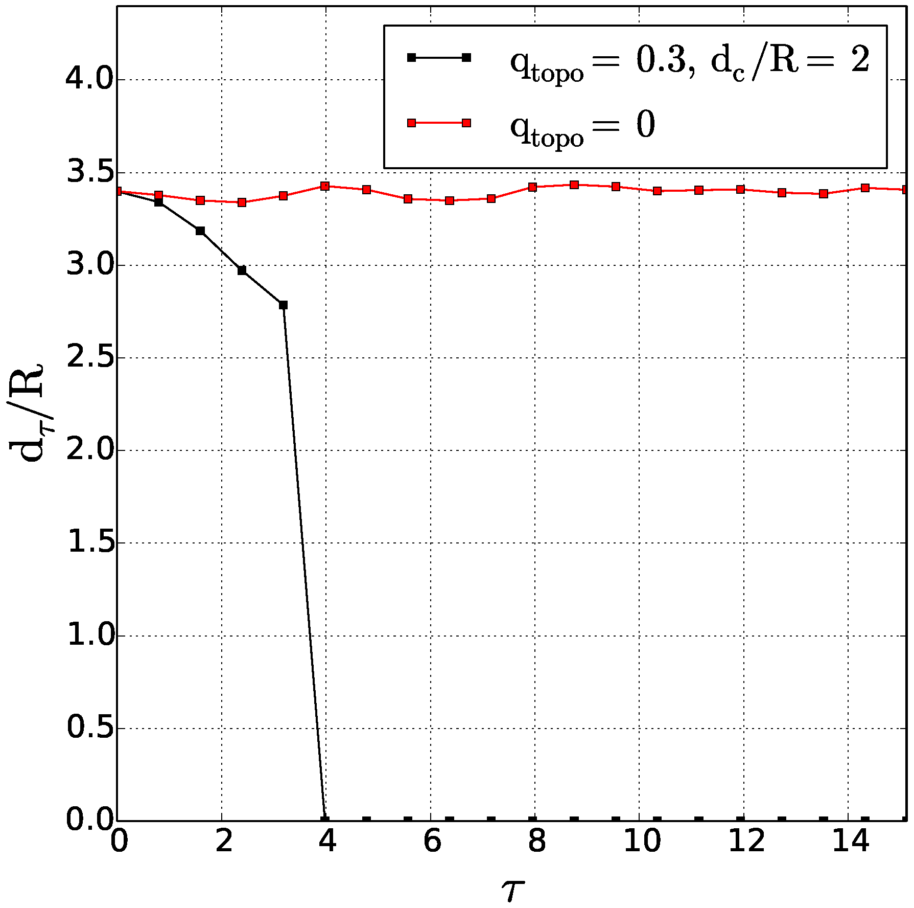
We study the interaction of two identical anticyclones, with $q_{topo}=0.3$. The regime diagram is presented in Figure 16. Compared with the interaction of two cyclones, two new regimes appear here; they are the drift of the two vortices away from the slope, without or with merger. In the case of merger, the critical distance can increase substantially, $d^{*}>7$, for $d_c/R=4$ (see an example of such a merger for two distant anticyclones in Figure 17).

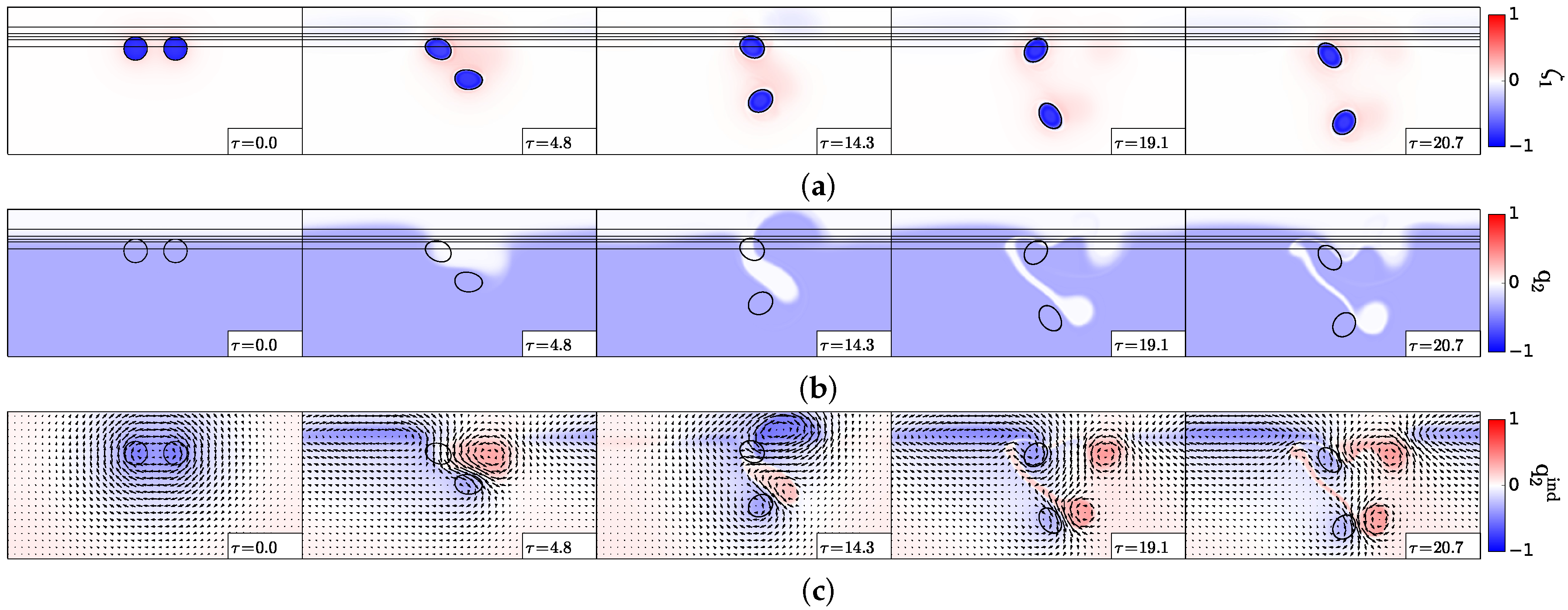
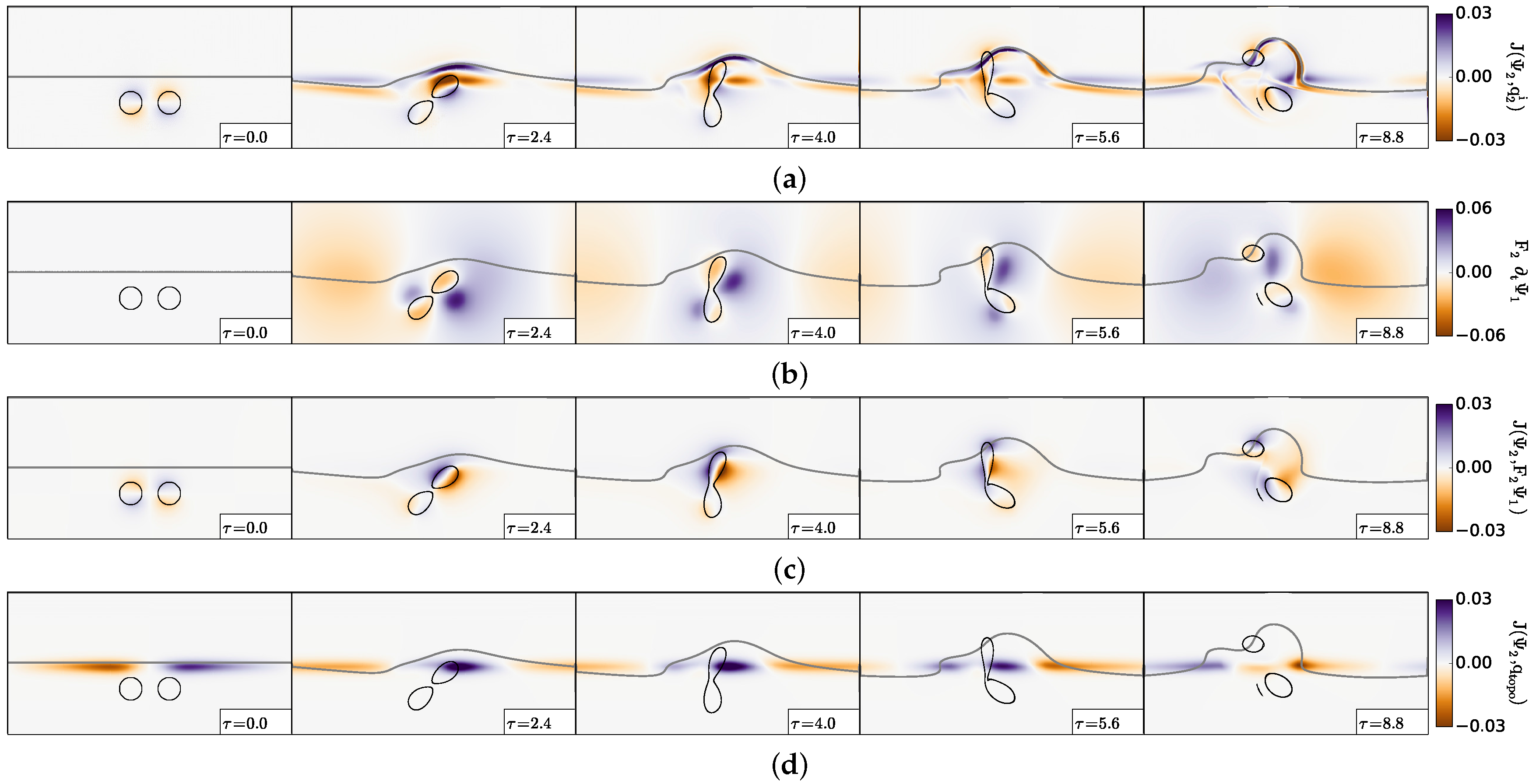
First, we present the drift of two anticyclones away from the slope for $d/R=3.4,d_c/R=1,\gamma R=1$ in Figure 18. In this regime, one anticyclone remains near the slope while the other one drifts away from the slope (see Figure 18a). This evolution is due to the coupling of this anticyclone with a positive potential vorticity pole in the lower layer (see Figure 18b,c). This lower cyclone separates the two upper anticyclones. The upper layer anticyclone close to the slope interacts successively with a lower layer cyclone and then with a lower layer anticyclone. The other upper layer anticyclone drifts offshore, coupled as a heton with a bottom cyclone.

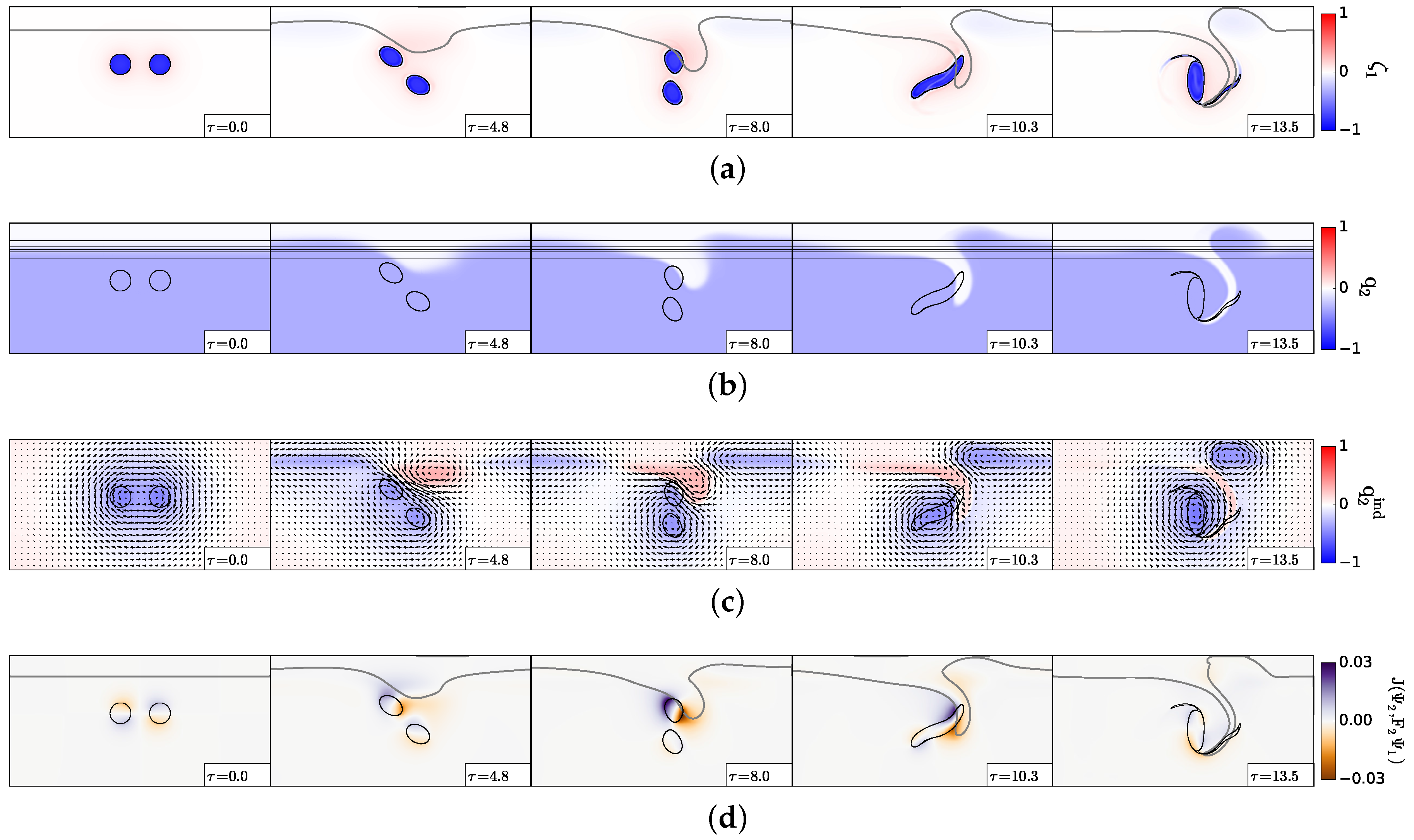
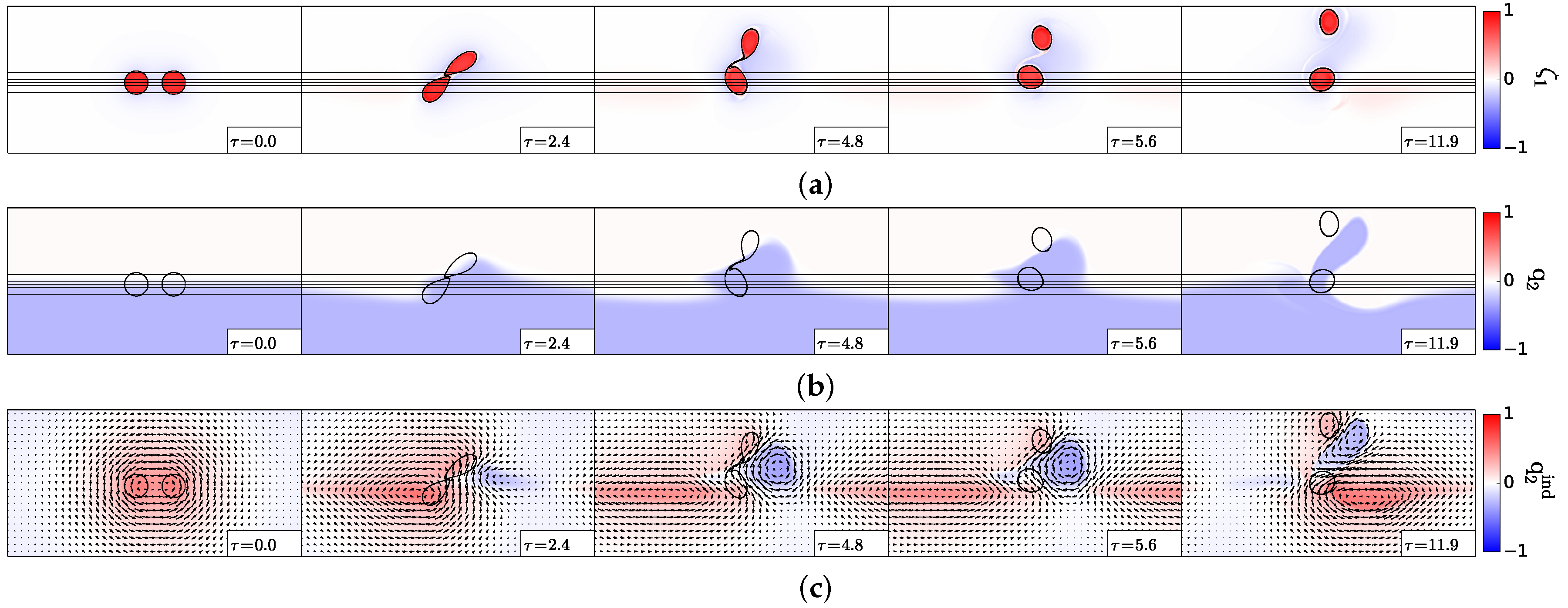
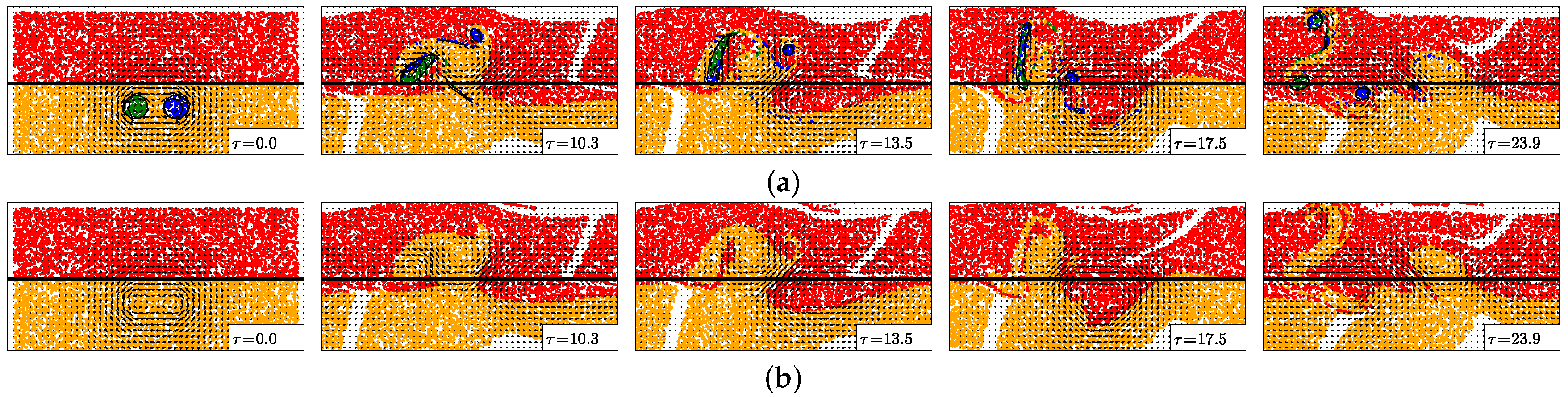
Next, we present the merger of two upper layer anticyclones, initially separated by $d=3.8R$, in Figure 19. The two upper layer anticyclones start rotating, and the westernmost one tears a filament of lower layer fluid offshore of the shelf (see Figure 19a,b). This lower layer filament couples with this upper layer anticyclone and advects it towards the easternmost anticyclone. Thus, the two anticyclones merge and shed filaments in the upper layer. The lower layer filament, which had been torn away from the shelf, then wraps around the merged anticyclone (see Figure 19b,c). The vertical coupling between layers (Figure 19d) is maximal between the westernmost anticyclone and the lower layer filament.

6. Evolution of Tracer and Particles across the Slope

The advection of the passive tracer and of the particles injected in the flow has been studied for all the regimes analysed above (for both the cyclones and the anticyclones). We next illustrate this advection during the interaction of two cyclones for the regimes of merger and splitting shown in Figure 8.

The tracer evolution, from the initial state with positive unit value in the deep region and negative unit value over the shelf, shows two essential patterns (see Figure 20):

(1)

The tracer distribution mostly follows the lower layer vorticity front initially; its gradient forms a double front, which also follows the vorticity filaments. This occurs in both layers (see Figure 20a,b). The concentration of tracer often occurs where the lower layer strain is intense and aligned with the tracer gradient (see Figure 20c).

(2)

There is considerable stirring of the tracer in the area where the two cyclones have merged, over the shelf (see again Figure 20a,b). This stirring is related to the intensity of the shear in this region.

Next, we analyse the time evolution of the particles initially seeded in both regions (shallow and deep) and in the vortex cores.

Results are presented in Figure 21 for both layers. Note that, due to the strong layer coupling in this case ($\gamma R=3.0$), the global pattern of particle evolution is similar in the two layers. The particles initially trapped in the cyclones are located only in the upper layer. Two main elements can be noted:

(1)

The particle evolution in the lower layer follows closely that of the tracer and of the lower layer potential vorticity, previously shown;

(2)

There are exchanges of particles between the two cyclones; the merged vortex contains particles from both of them, but with a majority of particles from the westernmost cyclone (that which is less deformed during the interaction). Similarly, the fragments (small vortex and filaments) mostly contain particles from the easternmost cyclone.

The number of particles crossing the slope inwards and outwards, in both layers, is shown in Figure 22. This number is maximal as the vortices cross the slope and merge. Then, it decreases as the merged upper layer cyclone elongates above the shelf, away from the slope. The number of particles crossing the slope reaches a nearly uniform value as two cyclones finally drift along the slope. The rotation associated with these cyclones generates a constant flux of particles in and out of the shelf.

7. Discussion and Conclusions

We have analysed the impact of a bottom slope on the interaction of two vortices (potential vorticity anomalies) located in the upper layer of a two-layer quasi-geostrophic model. The cases of cyclones and of anticyclones were successively addressed.

In the presence of a bottom topography of moderate height, but lying initially far away from the slope, two cyclones merge only for $d/R<3.3$ as above a flat bottom. However, then, they do not simply co-rotate around a fixed point; they also drift along the slope. An approximate steady state analytical solution was provided, which also shows that a large-scale deviation of the potential vorticity front appears over the topography. This was confirmed by numerical results.

When the two cyclones lie initially closer to the slope, the influence of the bottom topographic wave and vortices is more intense and leads to new dynamical regimes: asymmetric merger, splitting or drift towards the shelf. Asymmetric merger results from the different evolution of the two cyclones in their initial stage, as they co-rotate near the slope. The easternmost cyclone is elongated and can split into two parts, one of which can merge with the westernmost cyclone. Vortex elongation results from the shear induced by the bottom (topographic) vortices. A simple and approximate analytical model to assess the strength of this shear and the possible cyclone splitting is provided in Appendix B.

Globally, as the two cyclones are positioned initially closer to the slope, their critical merger distance increases, except when the two vortices lie exactly above the slope axis. Then, vortex separation can occur, again due to coupling with lower layer topographic vortices.

When the bottom topography is taller, two other regimes are observed, namely vortex drift and splitting, filamentation and asymmetric merger. The former occurs when the two cyclones are initially close to the slope, and it is due to the shearing effect of the bottom topographic vortices. The latter occurs when the two cyclones initially lie above the slope axis. It is a complex process by which the cyclones, being initially elongated, split; but all resulting fragments remain close to one another and finally merge together.

The interaction of two anticyclones brings about two other regimes, the drift of the two cyclones away from the slope, with or without merger. This drift is due to the tearing of a positive vorticity pole from the slope in the lower layer. This deep cyclone couples with one or both anticyclones and advects them away from the slope, as a heton. These results are qualitatively insensitive to horizontal resolution and to the choice of hyperviscosity, as long as the vortex profile is not altered by viscous effects.

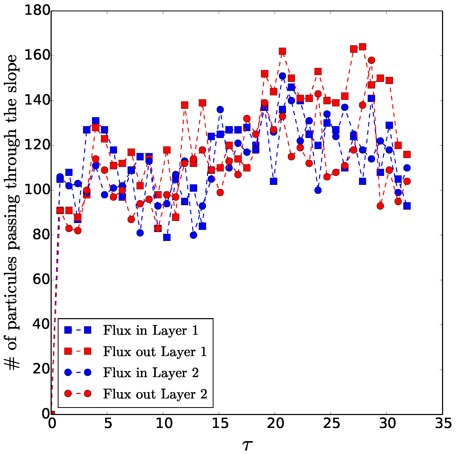
Finally, the evolution of tracer closely follows that of the potential vorticity. In the lower layer, the tracer is mixed in the region of vortex merger, while tracer fronts follow the strong gradients of potential vorticity, in particular the filaments. Based on the experiments, the fluid (or tracer) from the deep domain can easily be advected onto the shelf and be efficiently mixed there by the two-cyclone interactions. On the other hand, the interaction of two anticyclones, remaining essentially in the deep domain, is less efficient in advecting offshore fluid from the shelf, except if the two anticyclones are initially very close to the shelf break (a radius away).

Note that there is similarity between these results and vortex merger near a bottom slope in a homogeneous fluid, with quasi-2D dynamics [28]. The cyclones drift shorewards, and the anticyclones’ offshore and vortex merger are favoured (in particular asymmetric vortex merger). However, 2D dynamics allows less complexity in dynamical regimes and has a simpler dynamical mechanisms due to the absence of stratification. The present results also bear similarity with those of a previous study of vortex merger on the beta-plane [38], in that it also showed regimes of asymmetric vortex merger for two vortices initially more distant than $3.3R$. This was explained in that case by the beta drift of the two vortices, which could bring them close to each other, and by the energy loss by the vortices to the Rossby wave field.

Though this study already provided new results, it will have to be extended to address other important questions. Firstly, it would be interesting to use a quasi-geostrophic model with a finer vertical resolution (e.g., with three layers or with a continuous stratification) to evaluate the vertical deformation of the upper layer vortices during the interaction and also the three-dimensional structure of the deep potential vorticity poles. Note that secondary instabilities can then occur and split the vortices before they can interact; the results can be different [21].

Secondly, the case of very tall topographies (when the step height is comparable with the lower layer thickness) should be addressed with a primitive equation model. In this model, inertia-gravity waves and asymmetry between cyclone and anticyclone dynamics (the representation of which is banned by the geostrophic approximation in our model) may modify the present results. In particular, very tall topographies act as walls for the flow, associated with the influence of “ghost vortices” across the wall.

Associating both dynamical elements (primitive equation dynamics and fine vertical resolution) would allow the study of bottom boundary layers on the slope, which have been shown to generate submesoscale vortices [32].

Studying the interaction of smaller and more intense vortices than the mesoscale ones, that is vortices with $Ro\sim 1$ and/or $Bu\sim Ro$, would provide even richer phenomenology, including strong topographic vortices able to break the initial vortices, strong dependence to the vertical location of the initial vortex cores and again cyclone/anticyclone asymmetry in terms of stability or ability to interact (even in the absence of a shelf).

Lastly, this study will also have to be extended to reach the complexity of oceanic situations. Several dynamical elements will be added for oceanographic application: in particular, unequal layer thicknesses, capes or promontories in the shelf, the planetary beta effect, which supports planetary Rossby waves. All these effects can impact vortex merger near a coast as seen south of the Arabian Peninsula. However, it is presently difficult to make predictions from our simple study for oceanic situations with much larger complexity. This will be the subject of further studies.

References

1. Richardson, P.L.; Bower, A.S.; Zenk, W. A census of Meddies tracked by floats. Prog. Oceanogr. 2000, 45, 209–250. [Google Scholar] [CrossRef] [Green Version]
2. Carton, X. Hydrodynamical modeling of oceanic vortices. Surv. Geophys. 2001, 22, 179–263. [Google Scholar] [CrossRef]
3. Aguiar, A.C.B.; Peliz, A.; Carton, X. A census of meddies in a long-term high-resolution simulation. Prog. Oceanogr. 2013, 116, 80–94. [Google Scholar] [CrossRef]
4. Masina, S.; Pinardi, N. Merging of barotropic symmetric vortices. A case study for gulf stream rings. Il Nuovo Cimento C 1991, 14, 539–553. [Google Scholar] [CrossRef]
5. Schultz-Tokos, K.L.; Hinrichsen, H.H.; Zenk, W. Merging and migration of two meddies. J. Phys. Oceanogr. 1994, 24, 2129–2141. [Google Scholar] [CrossRef]
6. Carton, X.; Daniault, N.; Alves, J.; Chérubin, L.; Ambar, I. Meddy dynamics and interaction with neighboring eddies southwest of Portugal : Observations and modeling. J. Geophys. Res. 2010, 115. [Google Scholar] [CrossRef]
7. L’Hegaret, P.; Carton, X.; Ambar, I.; Menesguen, C.; Hua, B.L.; Chérubin, L.; Aguiar, A.; Le Cann, B.; Daniault, N.; Serra, N. Evidence of Mediterranean Water dipole collision in the Gulf of Cadiz. J. Geophys. Res. 2014, 119, 5337–5359. [Google Scholar] [CrossRef]
8. Overman, E.A., II; Zabusky, N.J. Evolution and merger of isolated vortex structures. Phys. Fluids 1982, 25, 1297–1305. [Google Scholar] [CrossRef]
9. Dritschel, D.G. The stability and energetics of corotating uniform vortices. J. Fluid Mech. 1985, 157, 95–134. [Google Scholar] [CrossRef]
10. Dritschel, D.G. The nonlinear evolution or rotating configurations of uniform vorticity. J. Fluid Mech. 1986, 172, 157–182. [Google Scholar] [CrossRef]
11. Carton, X. On the merger of shielded vortices. EPL (Europhysics Letters) 1992, 18, 697. [Google Scholar] [CrossRef]
12. Melander, M.V.; Zabusky, N.J.; McWilliams, J.C. Asymmetric vortex merger in two dimension: Which vortex is “victorious” ? Phys. Fluids A 1987, 30, 2610–2612. [Google Scholar] [CrossRef]
13. Melander, M.V.; Zabusky, N.J.; McWilliams, J.C. Symmetric vortex merger in two dimensions: Causes and conditions. J. Fluid Mech. 1988, 195, 303–340. [Google Scholar] [CrossRef]
14. Yasuda, I.; Flierl, G.R. Two-dimensional asymmetric vortex merger: Merger dynamics and critical merger distance. Dyn. Atmos. Oceans 1997, 26, 159–181. [Google Scholar] [CrossRef]
15. Yasuda, I.; Flierl, G.R. Two-dimensional asymmetric vortex merger: Contour dynamics experiments. J. Oceanogr. 1995, 51, 145–170. [Google Scholar] [CrossRef]
16. Meunier, P.; Ehrenstein, U.; Leweke, T.; Rossi, M. A merging criterion for two-dimensional co-rotating vortices. Phys. Fluids 2002, 14, 2757–2766. [Google Scholar] [CrossRef] [Green Version]
17. Griffiths, R.W.; Hopfinger, E.J. Coalescing of geostrophic vortices. J. Fluid Mech. 1987, 178, 73–97. [Google Scholar] [CrossRef]
18. Verron, J.; Valcke, S. Scale-dependent merging of baroclinic vortices. J. Fluid Mech. 1994, 264, 81–106. [Google Scholar] [CrossRef]
19. Valcke, S.; Verron, J. Interactions of baroclinic isolated vortices: The dominant effect of shielding. J. Phys. Oceanogr. 1997, 27, 524–541. [Google Scholar] [CrossRef]
20. Sokolovskiy, M.A.; Verron, J. Finite-core hetons: Stability and interactions. J. Fluid Mech. 2000, 423, 127–154. [Google Scholar] [CrossRef]
21. Von Hardenberg, J.; McWilliams, J.C.; Provenzale, A.; Shchepetkin, A.; Weiss, J.B. Vortex merging in quasi-geostrophic flows. J. Fluid Mech. 2000, 412, 331–353. [Google Scholar] [CrossRef]
22. Dritschel, D.G. Vortex merger in rotating stratified flows. J. Fluid Mech. 2002, 444, 83–101. [Google Scholar] [CrossRef]
23. Reinaud, J.N.; Dritschel, D.G. The merger of vertically offset quasi-geostrophic vortices. J. Fluid Mech. 2002, 469, 297–315. [Google Scholar] [CrossRef]
24. Reinaud, J.N.; Dritschel, D.G. The critical merger distance between two co-rotating quasi-geostrophic vortices. J. Fluid Mech. 2005, 522, 357–381. [Google Scholar] [CrossRef] [Green Version]
25. Bambrey, R.R.; Reinaud, J.N.; Dritschel, D.G. Strong interactions between two co-rotating quasi-geostrophic vortices. J. Fluid Mech. 2007, 592, 117–133. [Google Scholar] [CrossRef]
26. Ozugurlu, E.; Reinaud, J.N.; Dritschel, D.G. Interaction between two quasi-geostrophic vortices of unequal potential-vorticity. J. Fluid Mech. 2008, 597, 395–414. [Google Scholar] [CrossRef]
27. McDonald, N.R. The motion of an intense vortex near topography. J. Fluid Mech. 1998, 367, 359–377. [Google Scholar] [CrossRef]
28. Carton, X.; Morvan, M.; Reinaud, J.N.; Sokolovskiy, M.A.; L’Hegaret, P.; Vic, C. Vortex Merger near a Topographic Slope in a Homogeneous Rotating Fluid. Reg. Chaot. Dyn. 2017, 22, 455–478. [Google Scholar] [CrossRef]
29. Dunn, D.C.; McDonald, N.R.; Johnson, E.R. The motion of a singular vortex near an escarpment. J. Fluid Mech. 2001, 448, 335–365. [Google Scholar] [CrossRef]
30. Zhang, Y.; Pedlosky, J.; Flierl, G.R. Shelf Circulation and Cross-Shelf Transport out of a Bay Driven by Eddies from an Open-Ocean Current. Part I: Interaction between a Barotropic Vortex and a Steplike Topography. J. Phys. Oceanogr. 2011, 41, 889–910. [Google Scholar] [CrossRef]
31. Molemaker, M.J.; McWilliams, J.C.; Dewar, W.K. Submesoscale instability and generation of mesoscale anticyclone near a separation of the California Undercurrent. J. Phys. Oceanogr. 2015, 45, 613–629. [Google Scholar] [CrossRef]
32. Vic, C.; Roullet, G.; Capet, X.; Carton, X.; Molemaker, M.J.; Gula, J. Eddy-topography interactions and the fate of the Persian Gulf Outflow. J. Geophys. Res. 2015, 120, 6700–6717. [Google Scholar] [CrossRef]
33. Polvani, L.M.; Zabusky, N.-J.; Flierl, G.R. Two layer geostrophic vortex dynamics. Part 1. Upper layer V-states and merger. J. Fuid Mech. 1989, 205, 215–242. [Google Scholar] [CrossRef]
34. Gryanik, V.M. Dynamics of localized vortex perturbations on vortex charges, in a baroclinic fluid. Izv. Atmos. Ocean. Phys. 1983, 19, 347–352. [Google Scholar]
35. Gryanik, V.M. Dynamics of singular geostrophic vortices in a two-layer model of the atmosphere (ocean). Izv. Atmos. Ocean. Phys. 1983, 19, 171–179. [Google Scholar]
36. Hogg, N.G.; Stommel, H.M. The Heton, an Elementary Interaction Between Discrete Baroclinic Geostrophic Vortices, and Its Implications Concerning Eddy Heat-Flow. Proc. Royal Soc. A 1985, 397, 1812. [Google Scholar] [CrossRef]
37. Griffiths, R.W.; Hopfinger, E.J. Experiments with baroclinic vortex pairs in a rotating fluid. J. Fluid Mech. 1986, 173, 501–518. [Google Scholar] [CrossRef]
38. Bertrand, C.; Carton, X. Vortex merger on the beta plane. C. R. Acad. Sci. Paris Ser. II 1993, 316, 1201–1206. [Google Scholar]
39. Stern, M.E.; Flierl, G.R. On the interaction of a vortex with a shear flow. J. Geophys. Res. C 1987, 92, 10733–10744. [Google Scholar] [CrossRef]
Figure 1. Altimetric map showing the interaction of eddies near the east coast of Australia; notice the close interaction of two anticyclones near the coast (Archiving, Validation and Interpretation of Satellite Oceanographic Data altimetry).
Fluids 02 00057 g001
Figure 2. Sketch of model and vortex configuration; (a) side view; (b) top view.
Fluids 02 00057 g002aFluids 02 00057 g002b
Figure 3. Regime diagram for the interaction of two surface cyclones with: (a) given d c / R (see above each plot) in the γ R , d / R plane for f 0 h b 0 H 2 = 0.3 ; (b) given topographic vorticity (see above each plot) in the d / R , d c / R plane. Black stars indicate co-rotation; white stars represent co-rotation and drift along the shelf/slope; black squares indicate symmetric merger; black circles represent asymmetric merger; white circles denote asymmetric merger and vortex splitting; upward pointing triangles represent drift towards and on the slope and shelf; and triangles pointing left represent drift along the shelf/slope. The blue shading provides the value of the merger efficiency, when relevant.
Fluids 02 00057 g003
Figure 4. Critical merger distance d * , with respect to stratification, for various distances of the cyclone pair to topography.
Fluids 02 00057 g004
Figure 5. Partial merger of two cyclones, case d / R = 3.4 , γ R = 1 , d c / R = 2 . (a) Upper layer relative vorticity (Equation (3)); (b) lower layer potential vorticity (Equation (2)); (c) lower layer “equivalent barotropic” potential vorticity and velocity field (Equations (4) and (11)); (d) lower layer velocity shear (Equation (5)); (e) upper layer velocity shear (Equation (5)). In (a,b,d,e), the black contours indicate the topographic slope (Equation (12); straight lines) and the upper layer vorticity contours showing the two vortex evolution. In each plot, x varies between 2 π and + 2 π , and y varies between 0 and + 2 π .
Fluids 02 00057 g005
Figure 6. Partial merger of two cyclones, case d / R = 3.4 , γ R = 1 , d c / R = 2 . Analysis of the terms contributing to the rate of change of the lower layer “equivalent barotropic” potential vorticity (Equation (13)): (a) lower layer advection of this potential vorticity; (b) rate of change of the upper layer flow (via layer coupling); (c) baroclinic advection of the barotropic flow (with layer coupling coefficient); (d) interaction of the lower layer flow with the topography. In all sub-plots, the black contours indicate the front of lower layer potential vorticity anomaly (straight line at τ = 0 ) and the upper layer vorticity contours showing the two-cyclone evolution.
Fluids 02 00057 g006
Figure 7. Time evolution of the distance between cyclone centres for the partial merger of two cyclones; case d / R = 3.4 , γ R = 1 , d c / R = 2 ; comparison between the evolutions with and without the topography.
Fluids 02 00057 g007
Figure 8. Merger and splitting of two cyclones, case d / R = 3.4 , γ R = 3 , d c / R = 2 . (a) Upper layer relative vorticity (Equation (2)); (b) lower layer “equivalent barotropic” potential vorticity (Equation (11)); (c) lower layer velocity shear (Equation (5)); (d) upper layer Okubo–Weiss quantity (Equation (7)). The black contours indicate the topographic slope (Equation (12); straight lines) and the upper layer vorticity contours showing the two vortex evolution.
Fluids 02 00057 g008
Figure 9. Time evolution of the distance between vortex centres for the merger and splitting of two cyclones; case d / R = 3.4 , γ R = 3 , d c / R = 2 ; comparison between the evolutions with and without the topography.
Fluids 02 00057 g009
Figure 10. Separation of two cyclones, case d / R = 3.2 , γ R = 1 , d c / R = 0 . (a) Upper layer relative vorticity (Equation (3)); (b) lower layer potential vorticity (Equation (2)); (c) lower layer “equivalent barotropic” potential vorticity (Equation (11)). The black contours indicate the topographic slope (Equation (12); straight lines) and the upper layer vorticity contours showing the two vortex evolution.
Fluids 02 00057 g010
Figure 11. Fourier transform of the lower layer potential vorticity, on the slope, in the case d / R = 3.2 , γ R = 1 , d c / R = 0 . The modal coefficients a n ( t ) and b n ( t ) (Equation (15)) are plotted versus time, for several wavelengths λ = L / n = 4.0 π / n .
Fluids 02 00057 g011
Figure 12. Time evolution of the distance between vortex centres for the drift of two cyclones on the shelf; case d / R = 3.2 , γ R = 1 , d c / R = 0 ; comparison between the evolutions with and without the topography.
Fluids 02 00057 g012
Figure 13. Regime diagram for the interaction of two surface cyclones given d c / R (see above each plot), in the γ R , d / R plane, for f 0 h b 0 / H 2 = 0.6 . Black stars indicate co-rotation; white stars represent co-rotation and drift along the shelf/slope; black squares indicates symmetric merger; black circles represent asymmetric merger; white circles denote asymmetric merger and vortex splitting; triangles represent drift towards and on the slope and shelf; hexagons indicate filamentation and asymmetric merger; and crosses denote vortex drift and splitting. The blue shading provides the value of the merger efficiency, when relevant.
Fluids 02 00057 g013
Figure 14. Drift and splitting of two cyclones, case d / R = 3.6 , γ R = 2 , d c / R = 1 . (a) Upper layer relative vorticity (Equation (3)); (b) lower layer “equivalent barotropic” potential vorticity and velocity field (Equations (4) and (11)); (c) lower layer velocity shear (Equation (5)); (d) upper layer velocity shear (Equation (5)). In (a,c,d), the black contours indicate the topographic slope (Equation (12); straight lines) and the upper layer vorticity contours showing the two vortex evolution.
Fluids 02 00057 g014
Figure 15. Filamentation and asymmetric merger of two cyclones, case d / R = 3.6 , γ R = 2 , d c / R = 0 . (a) Upper layer relative vorticity (Equation (3)); (b) lower layer “equivalent barotropic” potential vorticity and velocity field (Equations (4) and (11)); (c) lower layer velocity shear (Equation (5)); (d) upper layer velocity shear (Equation (5)). In (a,c,d), the black contours indicate the topographic slope (Equation (12); straight lines) and the upper layer vorticity contours showing the two vortex evolution.
Fluids 02 00057 g015
Figure 16. Regime diagram for the interaction of two surface anticyclones, in the ( γ R , d / R ) plane, for fixed d c / R (for each sub-plot). Black stars indicate co-rotation. Black squares for symmetric merger; black circles for asymmetric merger and triangles for vortex drift, away from the slope (triangle pointing down) or along the slope (triangle pointing left).
Fluids 02 00057 g016
Figure 17. Merger of two anticyclones initially separated by d = 7.2 R for γ 3 , d c / R = 4.0 ; time series of the upper layer relative vorticity (Equation (3)).
Fluids 02 00057 g017
Figure 18. Drift of two anticyclones away from the slope for d / R = 3.4 , γ R = 1 , d c / R = 1 . (a) Upper layer relative vorticity (Equation (3)); (b) lower layer potential vorticity (Equation (2)); (c) lower layer velocity and “equivalent barotropic” potential vorticity (Equations (4) and (11)). In (a,b), the black contours indicate the topographic slope (Equation (12); straight lines) and the upper layer vorticity contours showing the two vortex evolution.
Fluids 02 00057 g018
Figure 19. Merger of two anticyclones away from the slope for d / R = 3.8 , γ R = 1 , d c / R = 3 . (a) Upper layer relative vorticity (Equation (3)); (b) lower layer potential vorticity (Equation (2)); (c) lower layer velocity and “equivalent barotropic” potential vorticity (Equation (11)); (d) Jacobian term of layer coupling F 2 J ( ψ 2 , ψ 1 ) . In (a,b,d), the black contours indicate the topographic slope (Equation (12); straight lines) and the upper layer vorticity contours showing the two vortex evolution.
Fluids 02 00057 g019
Figure 20. Tracer and strain evolution during the interaction of two cyclones for d / R = 3.4 , γ R = 3 , d c / R = 2 . (a) Tracer in the upper layer; (b) tracer in the lower layer; (c) strain field T 2 in the lower layer (Equation (6)). The black contours indicate the topographic slope (Equation (12); straight lines) and the upper layer vorticity contours showing the two cyclone evolution.
Fluids 02 00057 g020
Figure 21. Particle evolution during the interaction of two cyclones for d / R = 3.4 , γ R = 3 , d c / R = 2 . (a) Particles in the upper layer; (b) particles in the lower layer. The black contours indicate the topographic slope (Equation (12); straight lines) and the upper layer vorticity contours showing the two cyclone evolution.
Fluids 02 00057 g021
Figure 22. Number of particles crossing the slope inward and outward, in both layers, during the interaction of two cyclones for d / R = 3.4 , γ R = 3 , d c / R = 2 .
Fluids 02 00057 g022