The Impact of Topographic Steepness on Tidal Dissipation at Bumpy Topography

Abstract

Breaking internal waves are an important contributor to mixing in the stratified ocean interior. We use two-dimensional, nonhydrostatic numerical simulations to examine the breaking of internal waves generated by tidal flow over sinusoidal bottom topography. We explore the sensitivity of the internal wave breaking to the topographic steepness and Coriolis frequency, focusing on the vertical structure of kinetic energy dissipation and the ratio of local dissipation to the barotropic-to-baroclinic energy conversion. When the tidal frequency is twice the local Coriolis frequency, wave breaking above the topography is driven by wave–wave interactions which transfer wave energy from the tidal forcing frequency to the inertial frequency. The greater shear associated with the inertial frequency waves leads to enhanced dissipation in a thick layer above the topography. The topographic steepness strongly modulates this dependence of dissipation on Coriolis frequency; for some steep sinusoidal topographies, most wave energy propagates downward into the topographic troughs, eliminating the possibility for significant breaking above the topographic peaks. Current parameterizations of tidal dissipation in use in global ocean models need to be adapted to include the dependence of the local dissipation on both the Coriolis frequency and the topographic steepness.

1. Introduction

Tidal flow over sea-floor topography in a buoyancy-stratified ocean can lead to the generation of internal waves at the tidal frequency, also known as internal tides [1]. These waves propagate both vertically and horizontally, carrying wave energy away from their generation site [2]. When the waves break, that energy can be used for turbulent mixing of heat and salt. This mixing across density surfaces (diapycnal mixing) has an important role in large-scale ocean circulation, providing a mechanism for mixing heat down from the upper ocean, thereby lightening the deepest abyssal waters [3].

While internal tides are generated on horizontal scales of order 1–100 km, and break through overturning on much smaller scales, global climate models typically have resolutions of order 10–100 km, allowing resolution of the generation and propagation of only the large-scale internal tides and none of the wave-breaking and mixing processes [2]. The diapycnal mixing that results from internal tide breaking must therefore be parameterized. A parameterization commonly used in current climate models [4] represents this tidally-driven mixing in terms of the local dissipation of the internal tides near the generation site:

$$ϵ=\frac{qE(x,y)F\left(z\right)}{{\rho }_0}$$

(1)

where $ϵ$ is the turbulent kinetic energy dissipation, $E(x,y)$ is the energy transfer rate from the barotropic to the baroclinic tides as a function of horizontal coordinates $(x,y)$, q is the fraction of this tidal energy input used for dissipation (hereafter, dissipation fraction), $F\left(z\right)$ describes the vertical distribution of the dissipation, and ${\rho }_0$ is a reference density. The dissipation is then used to estimate the diapycnal diffusivity from [5],

$$\kappa =\frac{\Gamma ϵ}{N^2}$$

(2)

where $\Gamma$ is a mixing efficiency (commonly set to 0.2 [5]), and $N^2$ is the density stratification, given by

$$N^2=-\frac{g}{{\rho }_0}\frac{\partial \rho }{\partial z}$$

(3)

where $\rho$ is the density, z is the vertical coordinate, g is the acceleration due to gravity, and the square root of $N^2$ is the buoyancy frequency.

The energy conversion from the barotropic to baroclinic tide is parameterized using a simplified version of [6] from [7]:

$$E(x,y)=\frac{1}{2}{\rho }_0{N}_{b}k{h}_{\mathrm{rms}}^2\langle U^2\rangle$$

(4)

where $N_b$ is the value of N at the topography, k is the topographic wave-number, $h_{\mathrm{rms}}$ is the root-mean-square height of the topography, and $\langle U^2\rangle$ is the variance of the barotropic tidal velocity. To provide internal tide dissipation to climate models [8], Equation (4) is estimated using offline tidal models to calculate $\langle U^2\rangle$ [9] and gridded bathymetry datasets [10] to calculate k and $h_{\mathrm{rms}}$. $N_b$ is diagnosed from the temporally and spatially varying climate model fields. Much recent research has focused on improving this estimate of energy conversion to include the effects of finite amplitude topography [11,12,13].

In addition to assuming constant $\Gamma$, current implementations of this parameterization assume a constant dissipation fraction (q), set to 0.3, while observations [14] suggest that q can vary between 0.2–1.0. Understanding the physical mechanisms that determine spatial variations in q is an ongoing research problem.

The vertical distribution function $F\left(z\right)$ in current implementations has the form

$$F\left(z\right)=\frac{e^{-z/z_s}}{z_s(1-e^{-H/z_s})}$$

(5)

where z is the height above the bottom, H is the total ocean depth, and $z_s$ is a decay scale, set to a constant value (300–500 m in current global models) [4]. An alternative parameterization [15] has an algebraic decay function for dissipation, with a decay scale that varies according to physical parameters including stratification, tidal flow speed, and topographic height.

A numerical study [16] demonstrated that the ocean is sensitive to the vertical distribution of $ϵ$, highlighting the need to better constrain $F\left(z\right)$. Observations and numerical studies have both noted that processes such as hydraulic jumps [17,18,19] and nonlinear wave–wave interactions [20,21,22,23] can increase the magnitude of $ϵ$ and q, and alter $F\left(z\right)$ from the vertical profile in Equation (5) [4,15]. Nonlinear wave–wave interactions have been shown to be sensitive to Coriolis frequency [23], while tidally-driven hydraulic jumps have been shown to be sensitive to topographic steepness [17]. Our goal here is to improve the representation of tidal dissipation at the internal tide generation site by determining the dependence of q and $F\left(z\right)$ on the combination of sea-floor geometry and Coriolis frequency.

Internal waves are characterized by the dispersion relation

$$\omega =\sqrt{\frac{N^2{k}^2+f^2{m}^2}{k^2+m^2}}$$

(6)

where k and m are the horizontal and vertical wave-numbers, $\omega$ is the wave frequency, equal to the tidal forcing frequency for internal tides, and f is the Coriolis frequency. For propagating waves, $\omega$ must lie between f and N.

For internal wave generation by tidal flow over topography, summarized in [1], an important controlling parameter is the relative steepness (or criticality) of the topography ($\gamma$). $\gamma$ is defined as the ratio of the maximum topographic slope and the internal wave slope at tidal frequencies,

$$\gamma =\frac{{|\nabla h|}_{max}}{s}$$

(7)

where h is the height of the topography, s is the internal wave slope:

$$s=\frac{k}{m}=\sqrt{\frac{{\omega }^2-f^2}{N^2-{\omega }^2}}$$

(8)

which from the dispersion relation, Equation (6), is the slope of the group velocity vector relative to the horizontal. For subcritical topographies ($\gamma <1$), the internal wave slopes are steeper than topographic slopes. Therefore, since the group velocity vector (and hence direction of energy propagation) is aligned with s, the waves can only propagate upward, away from the bottom [1]. At critical slopes ($\gamma =1$), the internal waves have the same slope as the topography, so the wave energy becomes concentrated along the topography [24]. For supercritical topographies ($\gamma >1$), the internal wave slopes are less steep than the topographic slopes, and the wave energy can propagate both up and down the water column [12]. Critical slopes are known to be regions of enhanced dissipation [24], but the full impact of topographic steepness on dissipation at the generation site is not known.

Internal wave dissipation can be modified by wave–wave interactions which are in turn sensitive to the Coriolis frequency. Like all fluid motions, internal waves can undergo nonlinear interactions forming triads that satisfy

$${\mathbf{k}}_1={\mathbf{k}}_2+{\mathbf{k}}_3$$

(9)

$${\omega }_1={\omega }_2+{\omega }_3$$

(10)

where ${\mathbf{k}}_i$ are wave-number vectors and ${\omega }_i$ are frequencies [25]. For resonant interactions, the frequencies must satisfy the dispersion relation in Equation (6). For the particular subclass of triad interactions we consider here, parametric subharmonic instability (PSI) [26], the quantities with $i=1$ describe the initial wave, and the quantities with $i=2,3$ describe the resultant waves. From the dispersion relation, Equation (6), the resultant waves are freely propagating only for frequencies between f and N, which from Equation (10) requires $0<f\le {\omega }_1/2$. Following Equations (9) and (10), the wave energy can be transferred to smaller vertical length scales associated with greater shear. The PSI growth rate is enhanced when $f={\omega }_1/2$ [27], and this latitude has been shown observationally and numerically to be associated with greater dissipation [21,22,23]. At this latitude, the instability produces waves with frequency equal to f, and very large magnitude vertical wave-numbers, corresponding to small vertical wavelengths. Greater shear therefore results, leading to small Richardson numbers, where the Richardson number is defined as

$$Ri=\frac{N^2}{{(\partial u/\partial z)}^2+{(\partial v/\partial z)}^2}$$

(11)

where u and v are the horizontal velocity components. Linear theory [28,29] shows that stratified shear flows become unstable when $Ri<1/4$. This instability can transition to turbulence and hence leads to a transfer of energy to the small scales of dissipation [30].

PSI at the critical latitude can therefore initiate a transfer of energy from large-scale internal tides to dissipative scales, leading to enhanced dissipation. The known dependence of wave–wave interactions on f motivates us to explore how the Coriolis frequency impacts the dissipation of the internal tide.

The focus of our study is the breaking of internal tides near the generation site, where the generation occurs through tidal flow over sinusoidal topography. This topography is an idealization of the small-scale abyssal roughness found near ocean spreading zones, such as the Mid-Atlantic Ridge. Tidal mixing at realistic topography typical of the Mid-Atlantic Ridge has previously been examined in numerical simulations by [23], but the complex topography has complicated efforts to infer how q and $F\left(z\right)$ depend on topographic parameters. Our study therefore uses idealized topographies to determine the parameters which influence q and $F\left(z\right)$, using the Massachusetts Institute of Technology general circulation model (MITgcm) [31]. By focusing on idealized topography, we can examine the impact of topographic steepness on the wave-breaking processes and hence the dissipation profile. Topography with small horizontal scales is more likely to lead to internal tides with small vertical scales and high shear, and hence enhanced dissipation [32]. Here we will examine how the topographic steepness influences the roles that Coriolis frequency and topographic scale play in enhancing dissipation.

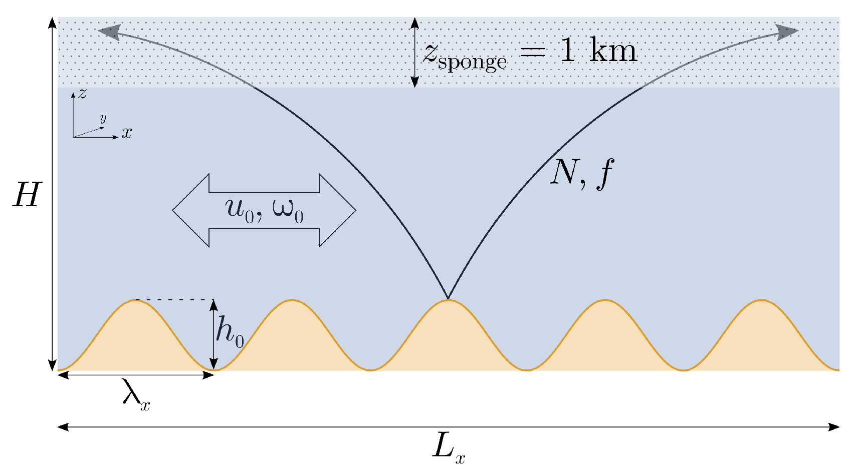
2. Methods

We use the MITgcm open source code [31], solving the nonhydrostatic, incompressible Navier-Stokes equations, to simulate the mixing driven by tides over rough topography. All simulations described here are carried out in two dimensions (a single horizontal and vertical directions), have constant initial density stratification and a linear equation of state, and employ periodic boundary conditions in the horizontal and a no-slip boundary condition at the topography. The Adams-Bashforth time-stepping scheme and centered second-order advection for both momentum and tracers are used.

The two-dimensional simulations of flow over one-dimensional topography are intended to approximate tidal flow over abyssal hill-like topographies [15,32,33]. The real abyssal hills are anisotropic, with greater topographic variation along one of the horizontal axes [34]. Since linear internal tide theory predicts that much of the tidal-energy conversion over these hills is supplied from the barotropic tidal flow along the direction with greater topographic variations [6,35], two-dimensional simulations are a reasonable first choice to examine this topography while minimizing computational cost.

In the real ocean, the interaction between upward propagating internal tides and variations in density stratification, particularly in the pycnocline, can lead to nonlinear wave–wave interactions and subsequent dissipation [36]. However, our focus is on the nonlinear interactions near the bottom topography, well below the pycnocline, and hence we make the assumption of constant stratification, simplifying the interpretation. In subsequent investigations we will include the complexity of variations in stratification.

A schematic of the experimental setup is shown in Figure 1.

Table 1. Model domain specifications for the 2-D simulations.

$\mathbf{\Delta }\mathit{x}$ (m)	$\mathbf{\Delta }\mathit{z}$ (m)	$\mathbf{\Delta }\mathit{t}$ (s)	${\mathit{L}}_{\mathit{x}}$ (km)	H (km)	$\mathit{\nu }$ (${10}^{-3}$ m${}^2/$s)	$\mathit{\kappa }$ (${10}^{-4}$ m${}^2/$s)
30	10	50	60	4	2	1

gives the values of numerical grid resolution and the Laplacian diffusion coefficients for momentum (viscosity $\nu$) and tracer (diffusivity $\kappa$), which are isotropic. Note that $\nu$ and $\kappa$ are constants, and not directly dependent on Richardson number or flow parameters. The fine spatial resolution and the nonhydrostatic configuration help resolve the shear instabilities that facilitate wave breaking [23].

The internal waves are generated by a lunar semidiurnal ($M_2$) tidal forcing that is added to the x-momentum equation:

$$F_{M_2}={\rho }_0{u}_0{\omega }_{0}cos\left({\omega }_{0}t\right)$$

(12)

where $u_0$ and ${\omega }_0$ are the $M_2$ tidal amplitude and forcing frequency, respectively. The tidal forcing frequency is set to $1.4\times {10}^{-4}$ s${}^{-1}$. We focus solely on the $M_2$ tide because it is the primary source of the tidally-driven mixing [3,8]. We add a one-kilometer sponge layer on top to damp the waves that reach the surface. Therefore, all the kinetic energy dissipation in our domain arises from waves that both are generated and break near the topography.

The topographies are generated as

$$h\left(x\right)=\frac{h_0}{2}\left[1+cos\left(\frac{2\pi x}{{\lambda }_x}-\pi \right)\right]$$

(13)

where $h_0$ is the peak-to-trough topographic height, and ${\lambda }_x$ is the horizontal wavelength of the topography. Finally, using the definition of relative steepness from Equation (7) with Equation (13), the peak-to-trough topographic height is related to $\gamma$, ${\lambda }_x$, and s by

$$h_0=\frac{\gamma s{\lambda }_x}{\pi }$$

(14)

We find the internal wave slope by setting the forcing frequency in Equation (8) to the $M_2$ tidal frequency ($\omega ={\omega }_0$).

Table 2. Parameter sets for different experiments.

$\mathit{f}\left({10}^{-5}{\mathbf{s}}^{-1}\right)$	${\mathit{\lambda }}_{\mathit{x}}$ (km)	$\mathit{\gamma }$	${\mathit{u}}_0$ (${10}^{-2}$ m/s)	${\mathit{N}}^2$ (${10}^{-6}$ s ${}^{-2}$)
$[0,5.3,7,10]$	$[2.5,3.75,6,8.57,12,15]$	$[0.68,1,1.71,4]$	$2.5$	1
$[0,7,10]$	6	$[1.3,2.4,2.8,3.4]$	$2.5$	1

shows the values of f, ${\lambda }_x$, $\gamma$, $u_0$, and initial stratification $N^2$ used in our simulations. Note that whereas $u_0$ and $N^2$ are held fixed for all our experiments, f, ${\lambda }_x$ and $\gamma$ are varied independently. For four different values of $\gamma$ (0.68, 1.0, 1.7, 4.0) we carry out simulations for four different values of f and six different ${\lambda }_x$, giving a total of 24 simulations for each of these values of $\gamma$. Note that as ${\lambda }_x$ varies, $h_0$ must also vary in order to hold $\gamma$ fixed. Similarly, as f varies, the wave steepness s varies, and so $h_0$ must also be modified to keep $\gamma$ fixed. For an additional four values of $\gamma$ (1.3, 2.4, 2.8, 3.4) we carry out three simulations at different f, keeping ${\lambda }_x$ fixed at 6 km. Our study therefore comprises 108 simulations ($24\times 4+3\times 4$).

As shown in [1], the ratio of tidal excursion distance to topographic wavelength $u_0/\left({\omega }_0{\lambda }_x\right)$ is an important parameter for internal tide generation; when $u_0/\left({\omega }_0{\lambda }_x\right)>1$, the internal wave response becomes increasingly dominated by higher harmonics of the forcing frequency ${\omega }_0$. For our simulations, with $u_0=2.5\mathrm{cm}/\mathrm{s}$ and ${\omega }_0=1.4\times {10}^{-4}{\mathrm{s}}^{-1}$, the maximum value of this parameter is $0.07$, when ${\lambda }_x=2.5\mathrm{km}$, indicating that the internal wave response is dominated by the forcing frequency [35].

A common way to study turbulent flows is to take data after the time when the turbulent kinetic energy of the system saturates. While all of our simulations are initialized from a state of rest, the density stratification is not restored back to the initial values. Therefore, the stratification evolves in time, and the turbulent kinetic energy (TKE) never truly reaches a single statistical steady-state. Rather, we take the data after the wave–wave interactions have developed (henceforth, referred to as statistical steady-state). All tidally-averaged quantities are calculated over 16 tidal cycles after our definition of statistical steady-state, and where error-bars are given, these are estimated as the standard deviation of the 16 tidal-average values.

The explicit dissipation of TKE in the model is

$$ϵ(\mathbf{x},t)=\nu \nabla \mathbf{u}·\nabla \mathbf{u}$$

(15)

where $\nu$ represents the kinematic viscosity and $\mathbf{u}$ the velocities. Gradients are estimated numerically by centered differences. Additionally, vertical profiles of $ϵ$ are calculated by taking the horizontal average of Equation (15).

The explicitly resolved tidal-energy conversion rate in the model domain is calculated as:

$$\begin{array}{ccc}\hfill E\left(t\right)& =\hfill & {\int }_{x=0}^{x=L_x}{p}^{\prime }(x,z=h\left(x\right),t)U_{b}t(x,z=h\left(x\right),t)dh/dxdx\hfill \\ & =\hfill & {\int }_{x=0}^{x=L_x}{p}^{\prime }(x,z=h\left(x\right),t)w^{\prime }(x,z=h\left(x\right),t)dx\hfill \end{array}$$

(16)

where $L_x$ is the model domain’s width, $p^{\prime }(x,z=h\left(x\right),t)$ is the perturbation pressure along the sea-floor from the waves, $U_{b}t(x,z=h\left(x\right),t)$ is the horizontal barotropic velocity along the sea-floor, calculated from a companion barotropic simulation as in [37], and $dh/dx$ represents the topographic slope [37,38] (this equality follows from non-divergence). Pressure at the bottom is approximated by the bottom-most pressure value on the model grid.

The spatially-integrated dissipation fraction between two depths, $z_1$ and $z_2$, is calculated as

$$q=\frac{{\rho }_0{\int }_{z_1}^{z_2}{\int }_0^{L_x}\langle ϵ\rangle dxdz}{\langle E\rangle }$$

(17)

where the angular brackets denote a temporal average over tidal cycles.

3. Results

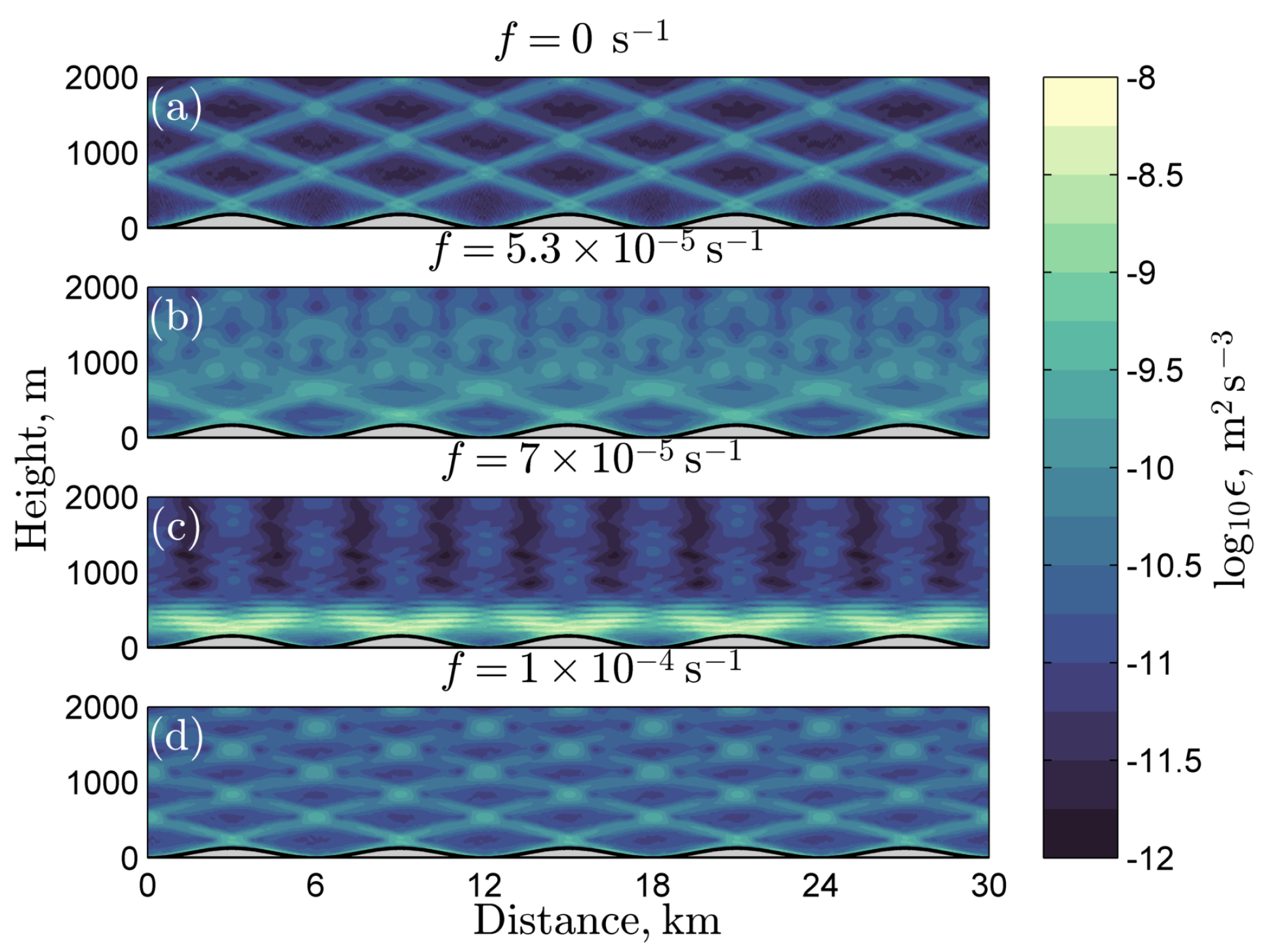
The influence of the Coriolis frequency on internal tide dissipation is demonstrated qualitatively in Figure 2, which shows the tidally-averaged dissipation of TKE ($ϵ$) for simulations where $\gamma =0.68$, ${\lambda }_x=6$ km, and f varies. Most of the dissipation in Figure 2a,d is contained within bands aligned with the internal tide characteristic slopes from Equation (8), which correspond to beams of internal tide energy propagating upward from the topographic peaks. The dissipation in panel b, however, is more spread out between $z=1000$ and 2000 m. The greatest dissipation among these four experiments is found in the bottom 500 m of panel c where $f={\omega }_0/2$, and ${\omega }_0$ is the $M_2$ tidal forcing frequency. The bands of high dissipation, which have small vertical scale and are closely aligned with the horizontal (the characteristic slope of inertial frequency waves, Equation (8)), are evidence for the efficient transfer of wave energy through resonant wave–wave interactions. The vertical scale of each of these bands of high dissipation is about 80 m, which is small compared to the topographic height, but nonetheless considerably greater than the model grid scale of 10 m.

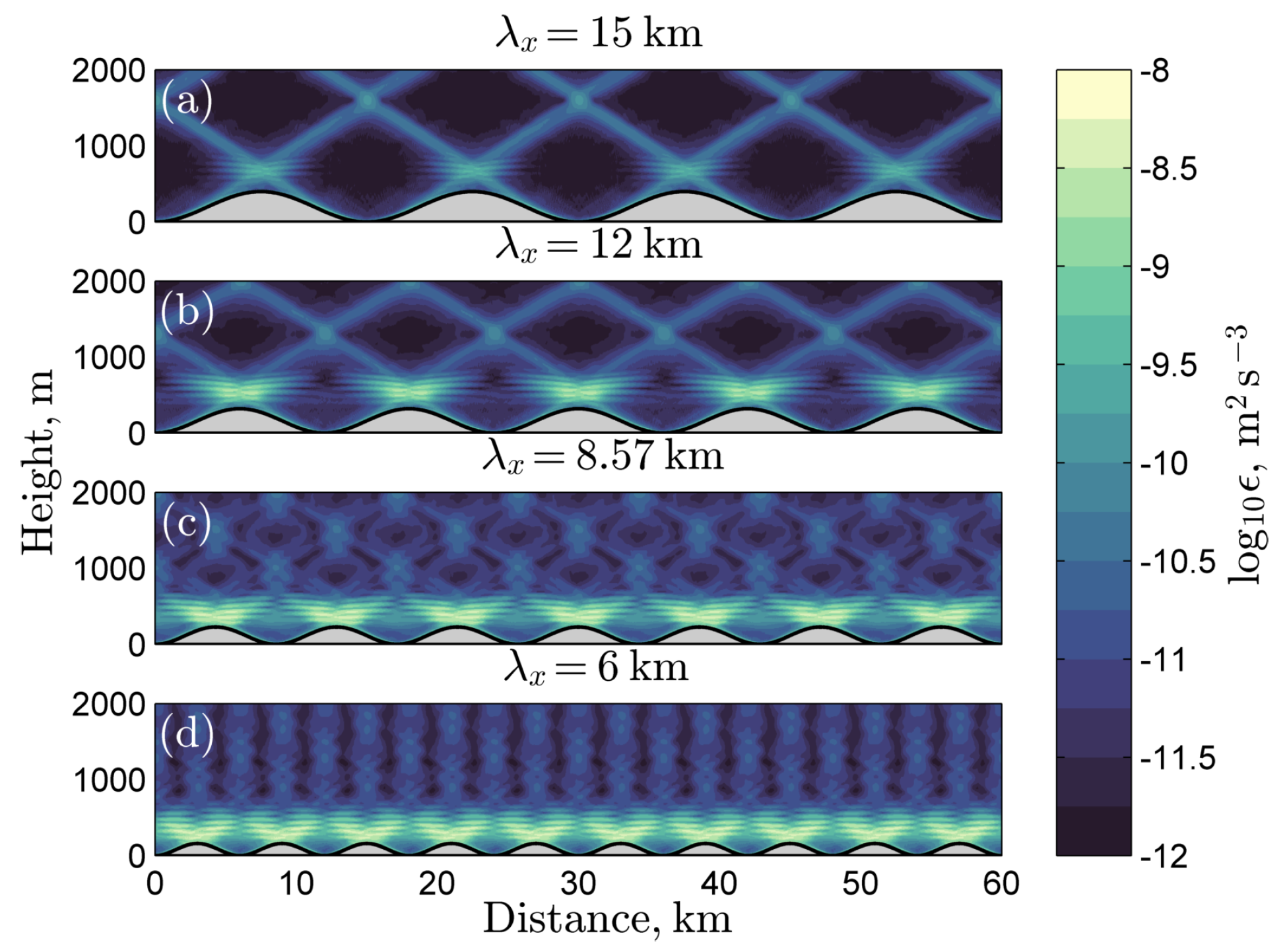
The wave breaking due to PSI is sensitive to topographic wavelength, as demonstrated in Figure 3, which shows tidally-averaged dissipation of TKE for simulations where $\gamma =0.68$, $f=7\times {10}^{-5}$ s${}^{-1}$, and ${\lambda }_x$ varies. Because all four experiments have $f={\omega }_0/2$, PSI features dominate the dissipation fields (seen in the small vertical length-scale regions of high dissipation aligned with the horizontal, above the topographic peaks in all panels). As the topographic length scale decreases, both the magnitudes and the fractions of the model domain’s horizontal extent that the PSI features occupy increase. This increase in dissipation with decreasing topographic wavelength is consistent with weakly nonlinear theory which predicts an increase in PSI growth rate for smaller wavelength internal waves [39]. For subcritical topography, the wavelength of the wave is set by that of the topography.

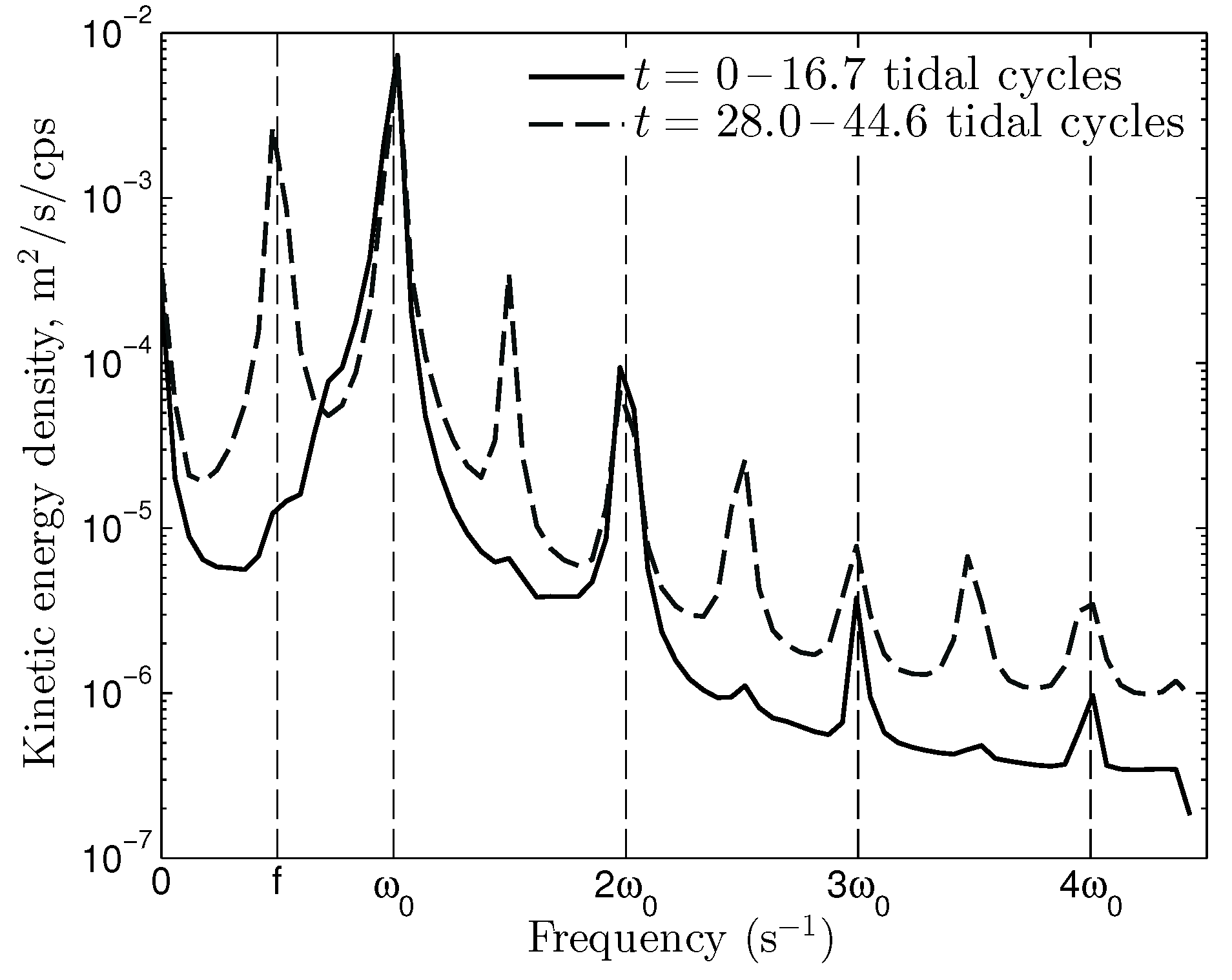
Figure 4 provides additional evidence for PSI at the critical latitude $f={\omega }_0/2$. Early in the simulation, the turbulent kinetic energy power spectrum is dominated by peaks at the forcing frequency ${\omega }_0$ and higher harmonics $n{\omega }_0$ (where n is a positive integer). Later in the simulation, a substantial amount of energy has been transferred to the inertial frequency f, and additional harmonic peaks at $f+n{\omega }_0$ are also seen.

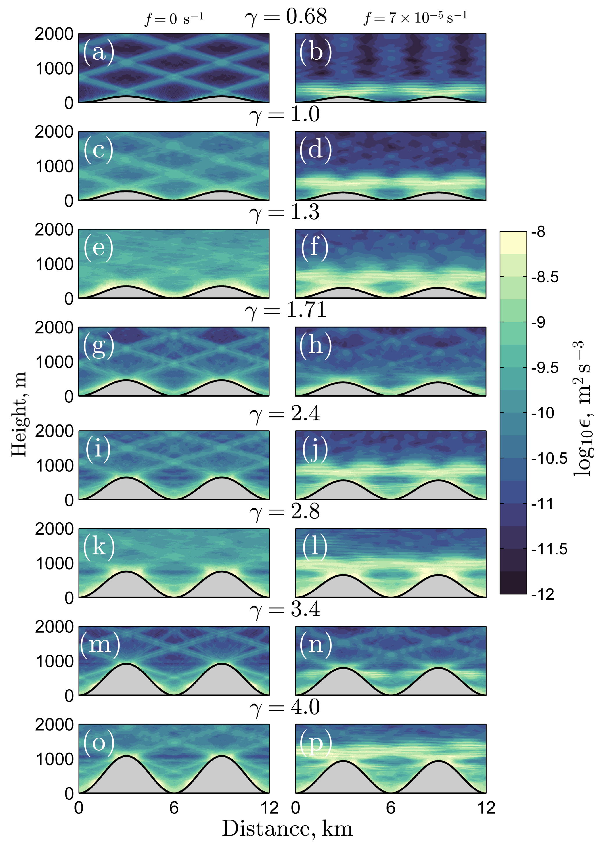
Having noted that PSI dominates the dissipation of the internal tide for $f={\omega }_0/2$, and the magnitude of this dissipation increases as the topographic length scale decreases for subcritical topography, we now examine the tidal dissipation as a function of increasing topographic steepness, $\gamma$. Figure 5 shows tidally-averaged $ϵ$ for two values of f and eight values of $\gamma$, all with the same ${\lambda }_x=6$ km. For $\gamma =1.71$ and $\gamma =3.4$ (Figure 5g,h,m,n), the overall dissipation of TKE seems to be qualitatively lower and confined mostly within the bottom boundary layer, and the wave–wave interactions are spatially smaller for $f=7\times {10}^{-5}$ s${}^{-1}$ (Figure 5h,n). For $\gamma =1.0$ (Figure 5c,d), $\gamma =1.3$ (Figure 5e,f), and $\gamma =2.8$ (Figure 5k,l), $ϵ$ is greater overall for both values of f when compared with $ϵ$ when $\gamma =0.68$ (Figure 5a,b). In particular, $\gamma =1.3$ and $\gamma =2.8$ for $f=7\times {10}^{-5}$ s${}^{-1}$ exhibit both the enhanced dissipation within the bottom boundary layer and the PSI features above the topography.

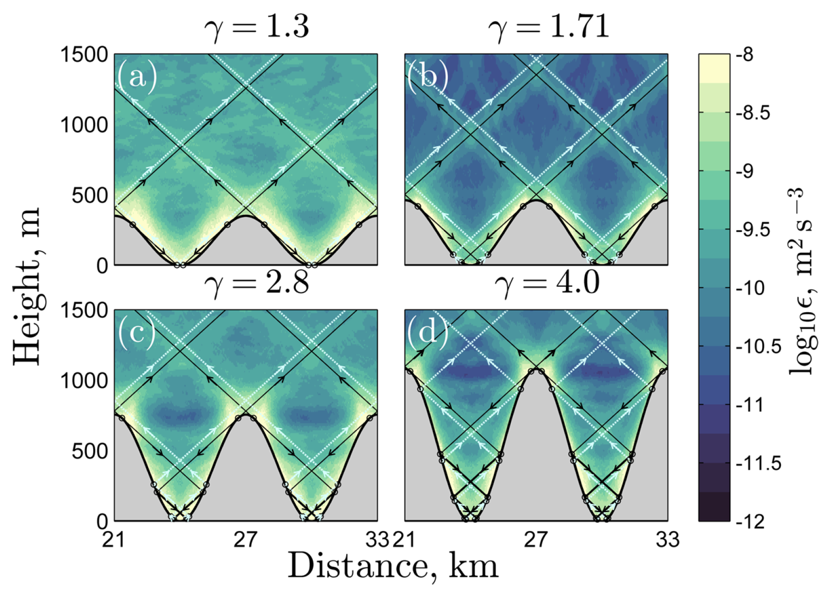
When topography is supercritical ($\gamma >1$), internal tide energy can propagate both upward and downward into the troughs between topographic peaks. These upward and downward internal tide characteristics, or ray paths, are shown in Figure 6, superimposed on the tidally-averaged energy dissipation for a subset of the supercritical simulations at $f=0$ (i.e., without PSI, so that most of the internal wave energy remains at the forcing frequency). The wave characteristics emanating upward and downward from the top of the slopes are co-located with regions of enhanced dissipation. Above the height of the topography, internal wave energy is carried upward not only by internal tide rays which were generated with upward group velocity at the top of the slope, but also by rays which originally had downward group velocity that ultimately reflected from the bottom topography. The number of reflections, how closely the rays are superposed, and the possibility for interference between upward and reflected rays are determined by the precise geometry of the topography, relative to the wave characteristic slopes.

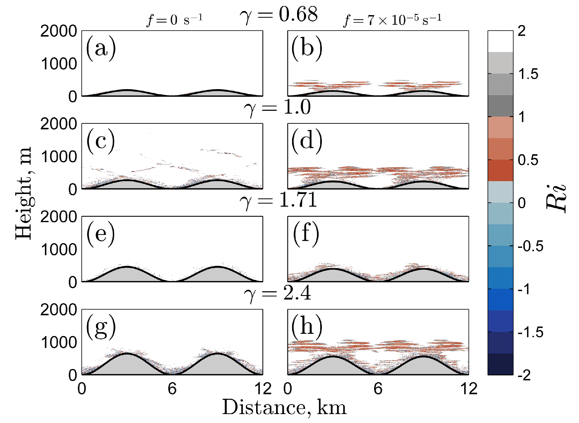
The mechanism leading to enhanced dissipation is demonstrated in Figure 7, showing the instantaneous Richardson number for two different values of f and four different values of $\gamma$. The instantaneous Richardson number allows us to highlight the transient regions of localized high shear and overturning associated with propagating waves. Areas of $Ri<0$ are associated with convective instability, while areas of $0<Ri<0.25$ satisfy the necessary condition for linear instability of a sheared stratified flow [28,29]. At $f=0$ the few regions of small $Ri$ are associated with the internal wave beams, (i.e., aligned with the internal wave slope, especially for critical topography, $\gamma =1.0$), and the troughs between the ridges of supercritical topography ($\gamma =1.71$, $2.4$). Subcritical topography ($\gamma =0.68$) has no regions of small $Ri$. At the critical latitude, $f=7\times {10}^{-5}$ s${}^{-1}$, the emergence of inertial frequency waves leads to large regions of small $Ri$, found well above the topographic peaks for $\gamma =0.68,1.0$, and $2.4$, but not for $\gamma =1.71$, where small $Ri$ continues to be concentrated in the troughs.

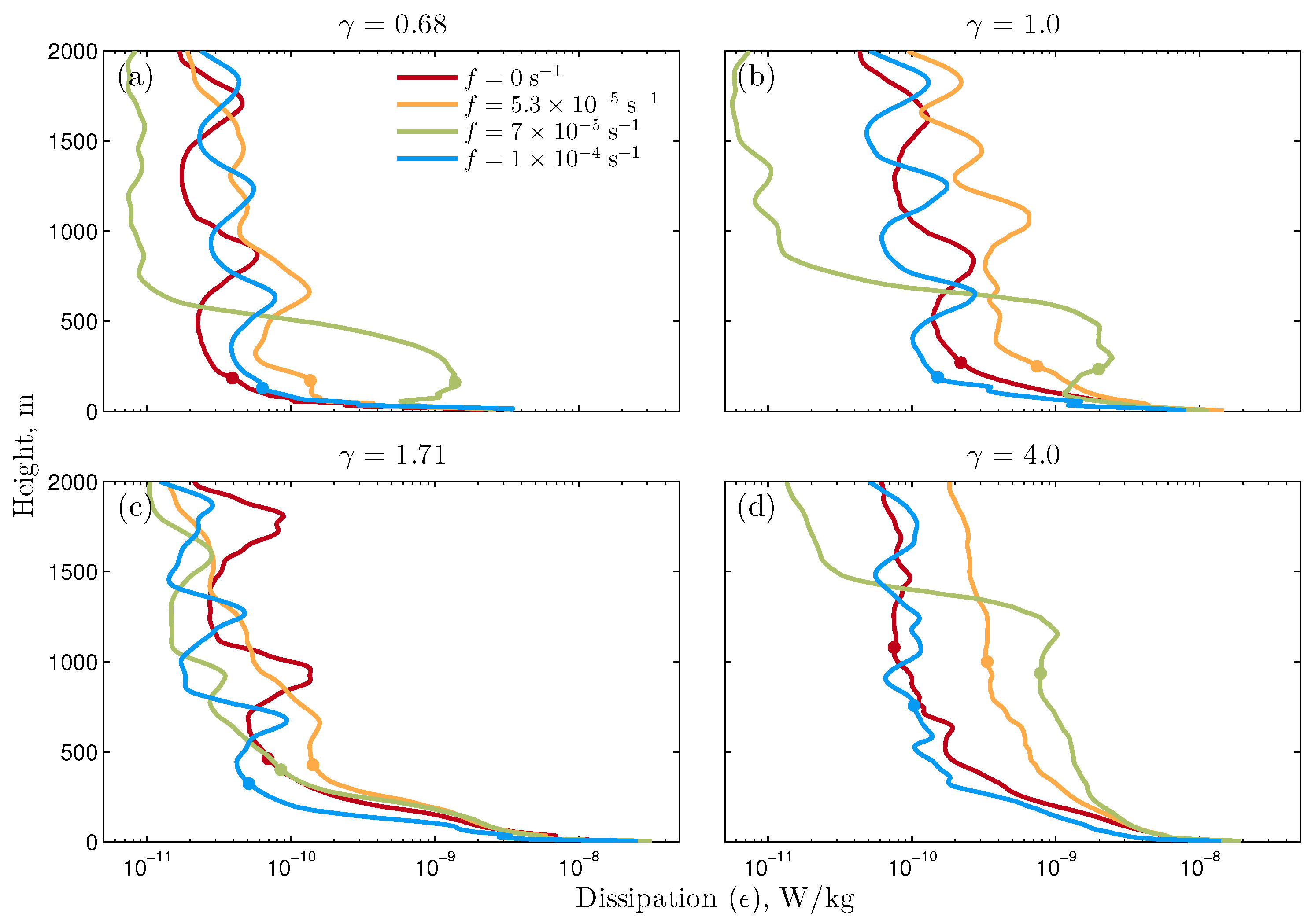
The impact of topographic steepness on dissipation due to wave–wave interactions generated as a function of latitude is summarized in the horizontally- and tidally-averaged profiles of dissipation shown as a function of height above bottom in Figure 8. All profiles show maximum dissipation at the topography and an overall decay with height above the topography. For $\gamma =0.68$ and $\gamma =1.0$, however, the dissipation does not decay monotonically with height; instead there is a marked increase in dissipation extending well above the bottom at $f=7\times {10}^{-5}$ s${}^{-1}$ compared to other values of f. For $\gamma =1.7$, the dissipation profile is much less sensitive to f, and the non-monotonic vertical profile is not seen at $f=7\times {10}^{-5}$ s${}^{-1}$. As previously seen in Figure 5 and Figure 7, this sensitivity to $\gamma$ is not monotonic, and at $\gamma =4.0$, dissipation is again enhanced well above the bottom for $f=7\times {10}^{-5}$ s${}^{-1}$.

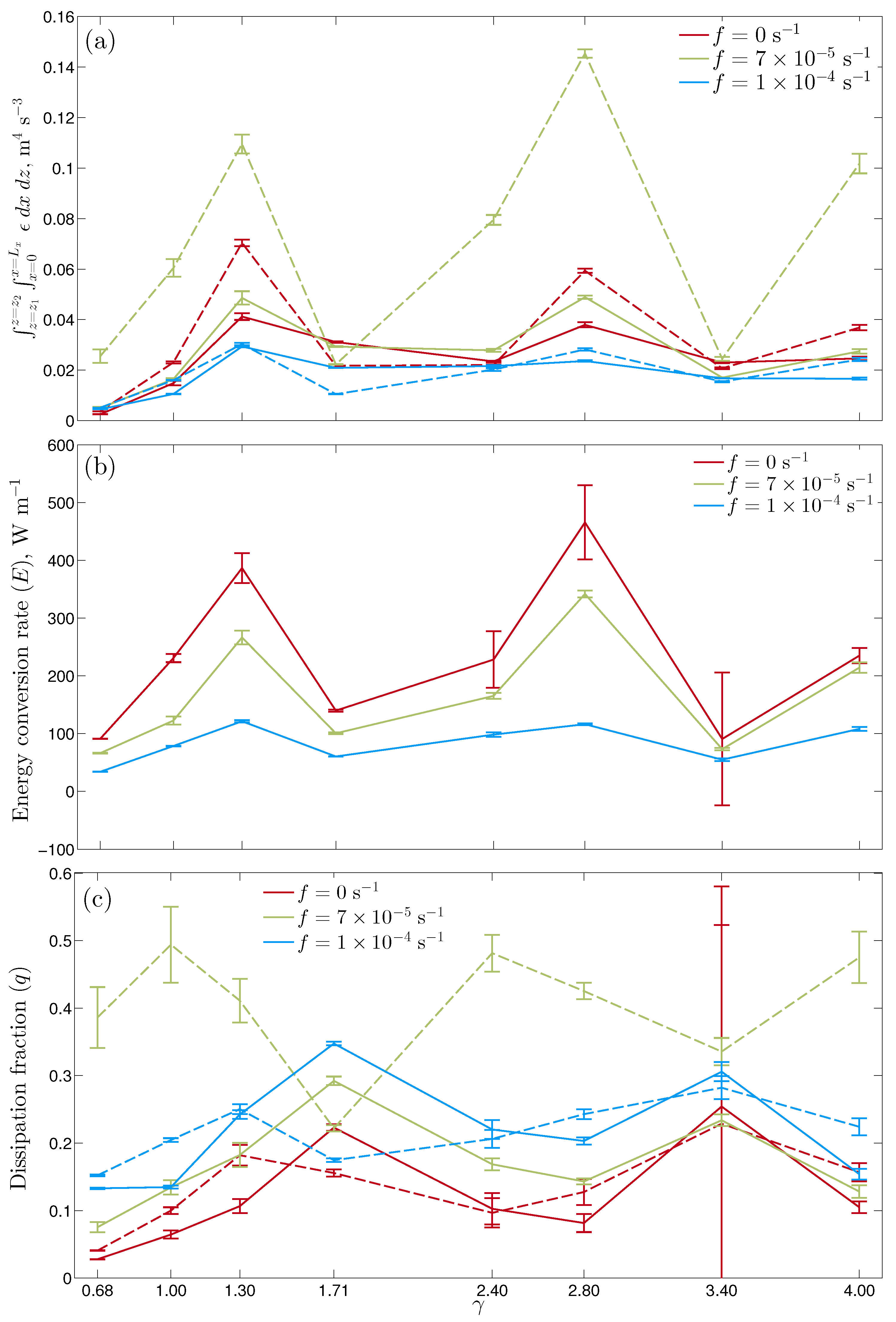
One possible cause of reduced dissipation at particular values of steepness could be a reduction in the energy conversion from barotropic to baroclinic motion, rendering less energy in the internal tide available to dissipate. Figure 9 shows the spatially-integrated dissipation ($ϵ$), tidal-energy conversion (E), and the spatially-integrated dissipation fraction (q) (the non-dimensional ratio of $ϵ$ to E). The solid lines are $ϵ$ values integrated from $z=0$ m to $z=50$ m above the bottom (which we define as the bottom boundary layer, bbl), and the dashed lines are values integrated from $z=50$ m to $z=2000$ m above the bottom. The choice of 50 m for the height of the bbl is somewhat arbitrary, but captures the dissipation occuring close to the topography. The Coriolis dependence of E can be explained approximately from [6], where $E\sim {\left({{\omega }_0}^2-f^2\right)}^{-1}$, so that E decreases monotonically with increasing f (Figure 9b). However, $ϵ$ does not show the same monotonic dependence on f; the highest integrated dissipation above the topography is found at $f=7\times {10}^{-5}$ s${}^{-1}$ (Figure 9a) where PSI occurs. Extrema in $ϵ$ above the topography are found at the same values of $\gamma$ as the extrema in E. The ratio q above the bbl is not constant and, for $f=7\times {10}^{-5}$ s${}^{-1}$, has minima at those values of $\gamma$ coinciding with minima in E (dashed lines in Figure 9c). By contrast, the integrated $ϵ$ in the bbl does not show a strong sensitivity to f, and only a weak sensitivity to $\gamma$, so that the nondimensional ratio q in the bbl peaks at those values of $\gamma$ where E is a minimum (solid lines in Figure 9c). The relative insensitivity of $ϵ$ in the bbl to f suggests that PSI is not the mechanism for transferring energy to small scales here. Instead, the tidal flow over the no-slip topographic boundary leads to a frictionally-driven shear layer. In summary, above the boundary layer, q is increased at the critical latitude where $f={\omega }_0/2$, but this increase is dependent on topographic steepness ($\gamma$). For those values of $\gamma$ where the energy conversion (E) is smallest ($\gamma =1.71$, $3.4$), q above the boundary layer is much less sensitive to f.

Theoretical models with finite amplitude topography and linear wave motion have previously been used [12,40] to show that the tidal-energy conversion rate behaves periodically as a function of $\gamma$. Our results show a similar quasi-periodic behavior, and like [12] we see a maximum in energy conversion at $\gamma =1.3$ and a minimum at $\gamma =1.7$. However for $\gamma >1.7$ we see a $\gamma =1.7$ periodicity in E, not the $\gamma =1$ periodicity seen in [12]. As a result, we see a maximum in energy conversion at $\gamma =2.8$, not a minimum as in [12]. Because this mismatch exists for all values of f, we eliminate wave–wave interactions as the cause. We hypothesize that the fully nonlinear waves generated in our simulations at larger $\gamma$, which for $\gamma >2$ include transient lee-waves as in [17], are the reason for this difference with the theoretical prediction.

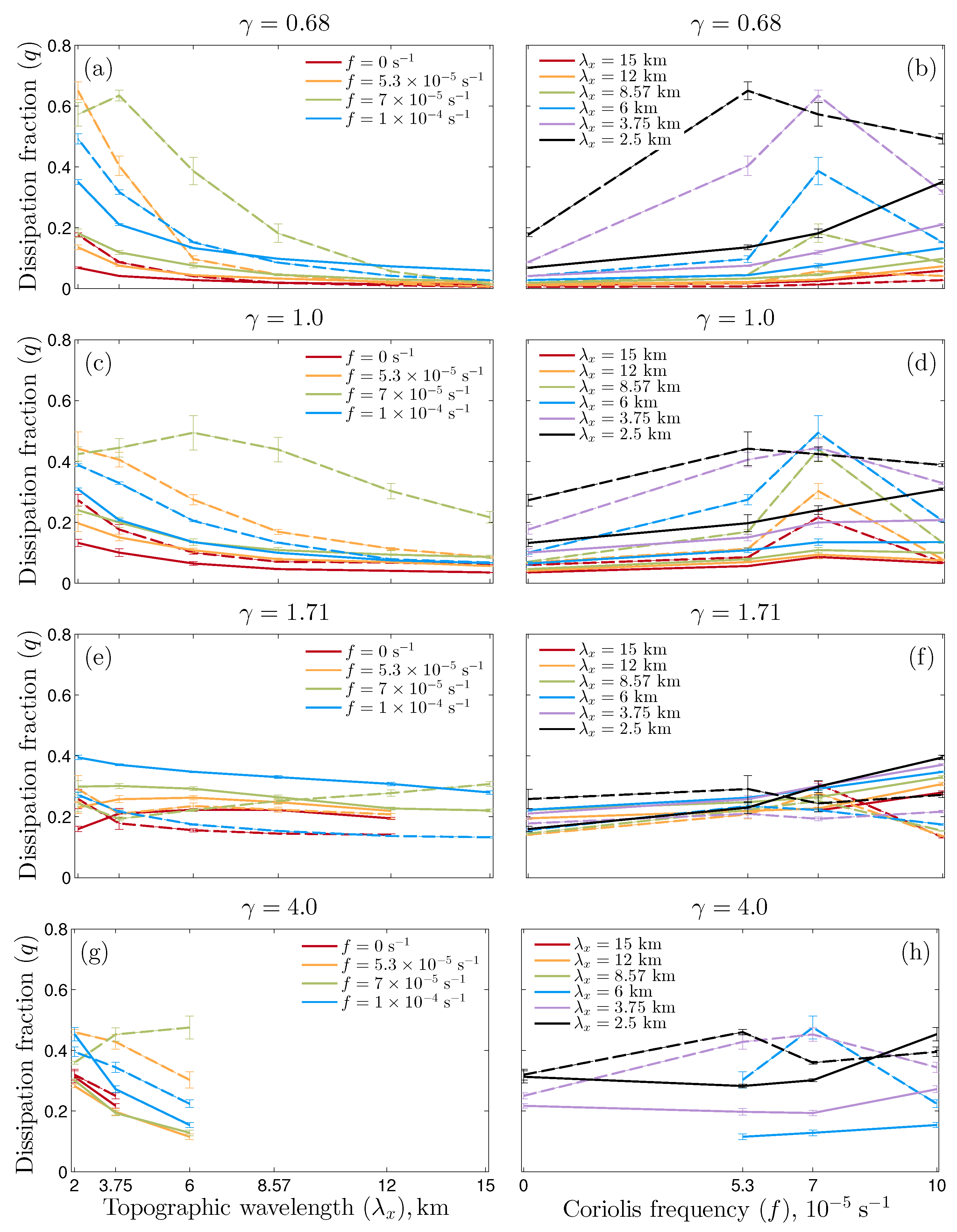
Figure 10 summarizes the non-dimensional ratio q in both the bottom boundary layer and above the topography as a function of topographic wavelength (${\lambda }_x$), Coriolis frequency (f) and topographic steepness ($\gamma$). For subcritical topography, $\gamma =0.68$, and critical topography, $\gamma =1.0$, q above the bbl peaks at the critical latitude $f=7\times {10}^{-5}$ s${}^{-1}$ and increases as ${\lambda }_x$ decreases. Within the bbl q is smaller and does not show a strong dependence on f. By contrast, for the supercritical case of $\gamma =1.71$, q above the bbl is much less sensitive to both topographic wavelength and Coriolis frequency, and approximately the same dissipation takes place in the bbl as in the region above. Wave–wave interactions, leading to enhanced dissipation above the topography at the critical latitude, are therefore inhibited for this particular value of $\gamma$, while they reappear at higher values of $\gamma$ (see the $\gamma =4.0$ results).

4. Discussion and Conclusions

Our analysis of these two-dimensional simulations of internal tide generation over sinusoidal bottom topography demonstrates that, as found in previous studies, the latitude of the generation site can influence the local dissipation. In particular, wave–wave interactions at or near the critical latitude, where $f={\omega }_0/2$, transfer energy from the tidal forcing frequency (${\omega }_0$) to the inertial frequency (f), associated with higher vertical wave-numbers, and hence lower Richardson number (Figure 7). The dissipation above the topography is then enhanced in a layer extending upwards well above the topographic peaks. Local dissipation fractions as large as $0.6$ result from this wave-breaking. Our new contribution has been to show that this Coriolis-dependent enhancement of local dissipation is highly sensitive to topographic steepness. Topographic steepness is known to influence the energy conversion at sinusoidal topography, with certain values of steepness leading to enhanced energy conversion through constructive interference between adjacent peaks, and other values of steepness leading to reduced energy conversion through destructive interference. In particular, as seen in [12], constructive (destructive) interference occurs when the initially downward propagating beam is reflected upward so that it has the same (opposite) phase as the adjacent beam propagating upward from the topographic peak. The phase is determined by the number of reflections from subcritical and supercritical slopes: at subcritical slopes, vertical velocity and buoyancy anomalies associated with the internal wave undergo a phase reversal, while at supercritical slopes, the phase of the vertical velocities and buoyancy anomalies are preserved after reflection. The geometry of the sinusoidal topography determines the nature of the reflections which occur in the troughs. As seen in Figure 6, at $\gamma =1.3$, there is one subcritical reflection of downward propagating waves. As a result, these waves reflect upward with a phase reversal, matching the phase of the upward going waves emanating from the next peak, and constructive interference occurs. For $\gamma =1.71$, there is one subcritical and one supercritical reflection. The downward, left propgating wave is reflected upward and rightward with a phase reversal. This reflected wave has the opposite phase to the rightward wave emanating from that peak, so destructive interference occurs. Buoyancy anomalies shown in [12] reinforce this interpretation of the constructive interference at $\gamma =1.3$ and destructive interference at $\gamma =1.71$.

Constructive interference tends to enhance energy conversion, while destructive interference reduces the energy conversion. We show here that those values of steepness with reduced energy conversion (e.g., $\gamma =1.71,3.40$) are also associated with greatly reduced dissipation above the topography, leading to reduced q above the topography, especially in comparison to the high values of q seen at $f=7\times {10}^{-5}$ s${}^{-1}$ for other values of $\gamma$. The reduction in q as the energy conversion is reduced is a consequence of the nonlinearity of the wave–wave interaction mechanism for dissipation. As a result, PSI is more rapid for more energetic wave fields, and a larger fraction of the tidal energy is transferred to higher modes and dissipated. A similar increase in q for larger energy conversion caused by constructive interference is seen in the lee wave-driven dissipation in the Luzon Straits double ridge system [41].

By contrast the dissipation in the bottom boundary layer is relatively insensitive to steepness, and q in the bottom boundary layer is actually enhanced for $\gamma =1.71$. Dissipation in this region is enhanced by frictional processes in the bottom boundary layer, and therefore more linear. For $\gamma =1.71$, as seen in the pattern of the wave beams in Figure 6, most of the downward propagating energy is confined near the slope, where the frictional dissipation dominates. The regions of reduced $Ri$ at $\gamma =1.71$ are similarly concentrated in the bottom of the troughs between topographic peaks. In contrast, for values of $\gamma$ where there is more upward energy propagation, the wave breaking and dissipation due to wave–wave interaction extend well above the topographic peaks, and are not related to friction at the boundary.

One limitation of this study is the restriction to two dimensions. In two dimensions, the barotropic tide forces fluid over the topography, while in three dimensions, fluid may flow around the topographic peaks. We have examined the impact of this effect with a small number of three-dimensional simulations with doubly sinusoidal topography with equal wavelengths in each horizontal direction. We find that when $f={\omega }_0/2$, features of parametric subharmonic instability again appear (not shown). However, the magnitude of energy conversion and dissipation are reduced for $\gamma =0.68$ and $1.0$, while both are increased for $\gamma =1.71$, consistent with the flow taking a less steep path over the topography. Real topography is likely to be anisotropic, leading to results intermediate between our two-dimensional and three-dimensional simulations.

Another limitation of our study is the use of values for viscosity and diffusivity which are greater than the molecular values for water, due to our finite numerical resolution. To explore the sensitivity to resolution and model viscosity parameters, we carried out a few simulations with coarser resolution and/or larger viscosity (not shown). While either very coarse resolution or large viscosity prevent the occurrence of PSI, for increases of order of a factor of two, we found the behavior to be unchanged. This suggests that provided PSI can be resolved, and is not damped, the dissipation is insensitive to the precise values of resolution and viscosity.

In summary, the vertical profile of dissipation and the ratio of local dissipation to energy conversion are both functions of the topographic wavelength, Coriolis frequency, and the topographic steepness. For subcritical topography, wave–wave interactions lead to an enhancement of dissipation at the critical latitude and for small wavelengths. By contrast, this sensitivity of dissipation profile to latitude and topographic wave-number is reduced for some steeper topography, when destructive interference reduces upward propagating wave energy, and dissipation occurs in the bottom boundary layer due to frictional processes. Future parameterizations of internal tide dissipation at rough topography generation sites should include the Coriolis dependence of the vertical profile of dissipation and the effect of topographic steepness on this Coriolis dependence. While parameterizations currently in use [4,15] prescribe a monotonic decay in dissipation with height, our results show that dissipation may vary with height non-monotonically at the critical latitude, depending on the topographic steepness.