Computational Fluid Dynamics Simulations of Gas-Phase Radial Dispersion in Fixed Beds with Wall Effects

Abstract

The effective medium approach to radial fixed bed dispersion models, in which radial dispersion of mass is superimposed on axial plug flow, is based on a constant effective dispersion coefficient, D_T. For packed beds of a small tube-to-particle diameter ratio (N), the experimentally-observed decrease in this parameter near the tube wall is accounted for by a lumped resistance located at the tube wall, the wall mass transfer coefficient k_m. This work presents validated computational fluid dynamics (CFD) simulations to obtain detailed radial velocity and concentration profiles for eight different computer-generated packed tubes of spheres in the range 5.04 ≤ N ≤ 9.3 and over a range of flow rates 87 ≤ Re ≤ 870 where Re is based on superficial velocity and the particle diameter d_p. Initial runs with pure air gave axial velocity profiles v_z(r) averaged over the length of the packing. Then, simulations with the tube wall coated with methane yielded radial concentration profiles. A model with only D_T could not describe the radial concentration profiles. The two-parameter model with D_T and k_m agreed better with the bed-center concentration profiles, but not with the sharp decreases in concentration close to the tube wall. A three-parameter model based on classical two-layer mixing length theory, with a wall-function for the decrease in transverse radial convective transport in the near-wall region, showed greatly improved ability to reproduce the near-wall concentration profiles.

1. Introduction

Fixed bed reactors are tubes filled with catalytic packing material, on which a chemical reaction may occur. Fixed bed reactors are preferred for their simplified technology and operation, and the design of such beds has been based on effective medium models coupled with correlation-based transport parameters. Low tube-to-particle diameter ratio (N) beds are typically selected for highly exothermic or endothermic reactions, such as in partial oxidations or hydrocarbon reforming. The use of larger particles within a tube of relatively small diameter results in a reduced pressure drop across the bed and, thus, a more economically-favorable operation. However, this results in a higher void fraction near the wall of the bed, which induces significant flow and transport effects that are difficult to account for in conventional packed bed models. In this near wall area, boundary layers develop in which heat and mass transfer are dominated by molecular transport, and a high resistance to transport is present, causing strong changes near the wall.

Dispersion is a phenomenon in which a solute in a porous medium spreads as a result of the combined effects of molecular diffusion and convection in the interstices or the space available for fluid flow between particles. Typical applications of dispersion are, for example, in quantifying contaminant transport in soils or in modeling solute transport in fixed beds. The study of dispersion in packed bed reactors is fundamental to their design in that dispersive phenomena characterize reactant and product transport within the bed [1,2,3,4]. Dispersion may be modeled analogously to Fickian diffusion by replacing the diffusion coefficients with dispersion coefficients as seen in the following partial differential equation for species concentration:

$$D_L\frac{{\partial }^{2}C}{\partial z^2}+\frac{1}{r}\frac{\partial }{\partial r}\left(D_{T}r\frac{\partial C}{\partial r}\right)-u\frac{\partial C}{\partial r}=\frac{\partial C}{\partial t}$$

(1)

In Equation (1), D_L is the axial or longitudinal dispersion coefficient and D_T is the radial or transverse dispersion coefficient, related to flow in the freestream and cross-stream directions, respectively. When dealing with dispersion, it is often useful to define dimensionless Péclet numbers, representing the ratio of advective to dispersive transport:

$$P{e}_T= \frac{v_i d_p}{D_T}$$

(2)

and:

$$P{e}_L= \frac{v_i d_p}{D_L}$$

(3)

where v_i is the interstitial velocity in the bed and d_p is the particle diameter.

The present study is focused on the transverse dispersion coefficient, rather than on the longitudinal coefficient. The latter is important for such applications as chromatography and the understanding of residence time distribution in fixed beds. Our main motivation for studying dispersion, however, is the analogy between convective heat and mass transfer, since radial heat transfer is one of the most important parameters in fixed bed modeling. Studies of mass dispersion can give insight into the modeling of fluid-phase convective heat transfer.

Strong radial temperature profiles are common in fixed beds of low N. In contrast, both random walk theory and early experimental results suggested that radial concentration profiles would be fairly flat, although radial dispersion near the tube wall could be reduced due to flow channeling there, leading to radial concentration profiles. Experimental studies of radial dispersion in fixed beds have been conducted for over 70 years (see, for example, [5,6,7]) and have for the most part been conducted by a centerline pulse injection of a tracer substance, with a small number of radial concentrations measured at the bed exit to avoid disturbing the bed packing [5,6,7,8,9]. These measurements are made on beds of relatively short length, before the solute has spread over the entire bed radius, to obtain non-uniform radial concentration profiles. The consequence is that for most studies, the wall effects are deliberately excluded, so as to obtain infinite-medium D_T values.

Opinions have been divided on whether there is a wall effect on fixed bed radial dispersion. An early study by Fahien and Smith [6] used a centerline point source, but allowed the dispersing solute to reach the tube walls. They found that D_T was not constant across the tube radius and that the decrease in D_T near the tube wall depended on the tube-to-particle diameter ratio, N. The authors correlated their results for radial average transverse dispersion coefficient by:

$$P{e}_T=\frac{8}{1+19.4/N^2}$$

(4)

Wall effects on transverse dispersion were also found in the presence of thermal gradients by Schertz and Bischoff [10] who attributed the effect to changes in fluid viscosity with temperature. Gunn and Pryce [8], on the other hand, found no wall effect, although their tracer did not reach the tube walls. Han et al. [9] also concluded that the values of D_T did not depend on bed location, as they were not time dependent in their transient study. Foumeny et al. [11] from tracer experiments with internal bed measurements at different bed heights suggested a correlation with a term that explicitly accounted for wall effects and remarked upon the unreliability of data taken from the bed exit, as the flow patterns change rapidly there, and upon the high correlation between the longitudinal and transverse dispersion coefficients in standard models.

In order to investigate the wall effects on dispersion and obtain wall transport coefficients that could be used in heat transfer studies by analogy, several research groups performed experiments in which the tube wall was coated with a dissolving substance [12,13,14,15,16,17,18,19]. A wall mass transfer coefficient was introduced, either through a modified boundary condition on Equation (1) [12,15,16,17,19] or by the theory for limiting current measurements in an electrochemical system [13,14,18]. A detailed understanding of the transport processes near the tube wall could not be obtained by these methods, due to the small number of radial concentration measurements that could be made.

In an experimental and modeling study, Coelho and Guedes de Carvalho [20] studied transverse dispersion in granular beds. They used a two-region plug-flow model in which a near-wall region of thickness δ may be thought of as a laminar sub-layer in which molecular diffusion is the dominant mechanism. Outside of this layer, the transport in the bed is due solely to dispersion. They performed experiments with a soluble wall for different bed lengths and obtained values of the overall mass transfer coefficient k_av to which they were able to fit the two parameters D_T and δ. Using these parameters, they were able to predict overall mass transfer coefficients for other values of Re and L with reasonable agreement. An interesting result of their work was that for a long enough bed, the δ-region saturates with the soluble species and a one-parameter model suffices. The criterion for a one-parameter model to be valid is:

$$\frac{L}{d_p}>0.625 \frac{Re·Sc}{\epsilon }$$

(5)

where $\epsilon$ is the bed voidage and Re is based on the interstitial velocity.

In following experimental studies, Guedes de Carvalho and Delgado [21,22] studied lateral dispersion in fixed beds of spheres by including in the bed a soluble cylinder of benzoic acid aligned with the flow of water entering the tube. They neglected any near-wall effects on dispersion, stating that the section of packing contacting the soluble slab actually indents onto this soluble section, removing the near-wall, high-voidage region that is typical in a fixed bed. Solute concentration in the outlet section of the bed was measured as a means to determine the rate of dissolution of the cylinder. Diffusion was treated as occurring in one dimension, given that the bed followed the criterion in Equation (5). The authors noted the strong dependence of D_T/D_m on Sc in the range 140 < Sc < 500 and showed that dispersion behavior was generally independent of particle size. In later work by Delgado [4], both longitudinal and transverse dispersion in porous media were studied over a wide range of the Schmidt and Péclet numbers. The author supplied a set of equations each for the longitudinal and transverse dispersion coefficients, subdivided by different regimes of dispersion based on the molecular Péclet number: (1) diffusion regime (Pe_m < 0.1); (2) predominant diffusional regime (0.1 < Pe_m < 4); (3) predominantly mechanical dispersion (4 < Pe_m and Re < 10); (4) pure mechanical dispersion (10 < Re, Pe_m < 10⁶); and (5) dispersion beyond the validity of Darcy’s law (Pe_m > 10⁶). While this paper presents important correlative equations for dispersion, the experimental data were largely from beds above the low N range (2 < N < 8). The difficulties of obtaining detailed experimental measurements in complicated systems such as fixed beds has suggested the use of computational tools as a complementary method of obtaining insight into transport properties such as dispersion.

Computational fluid dynamics (CFD) is a numerical method-based computing approach for simulating fluid flow, mass and heat transport and reaction kinetics, among other physical phenomena. In general, the use of CFD requires converting the geometry of interest, here a fixed bed of spheres, into a number of small control volumes, collectively called the computational mesh, or grid. After supplying the appropriate boundary conditions related to flow and species transport and an initial, estimated solution for the system of interest, a complete numerical solution can then be obtained by iterative, convergence-guided, numerical techniques. With the recent introduction of high performance computing capabilities and the continued growth of such computing resources, CFD can now be used as an important tool for the design and simulation of fixed beds. The use of CFD allows the elucidation of certain flow and heat characteristics that cannot be obtained from experimental methods, such as the velocity distribution around and between particles or the temperature at any point within the bed.

An early use of CFD to simulate flow and dispersion in computer-generated random sphere packs was made by Schnitzlein [23]. The motivation for the study was his observation that radial dispersion should be the sum of molecular diffusion and fluid mechanical phenomena (eddy diffusion in local voids, which act as mixing cells, branching in the packing and channeling due to the placement of particles and the wall effect) and should not be driven by a concentration gradient. This point of view was similar to one suggested by Gunn [1] who described axial and radial dispersion in terms of probability theory, accounting for dispersion in the fast stream (convective-dominated) and the slow stream near the tube wall (diffusion-dominated). Gunn estimated the probability of a particle existing in the diffusion boundary layer or moving into the fast stream area of the bed. He stated that diffusion in the bed had little effect on convective radial dispersion and introduced a fluid-mechanical Péclet number based on convective-dispersion alone, which in the limit of a high Reynolds number tended to 11.

In Schnitzlein’s work, a two-dimensional map of the void fraction was obtained from the computer-generated packing and used in the porous medium 2D Navier–Stokes equations to obtain a two-dimensional velocity field. The velocity field was then used in a 2D mass balance to generate a simulated dispersion experiment. This was then fit by a standard dispersion model to estimate D_T, which gave a limiting fluid-mechanical Péclet number of 28, which was probably due to low variation in local voidage, leading to underestimation of radial displacement of fluid. A second study by Schnitzlein [24] used the sphere pack to obtain a 3D network model with inertial terms, but no diffusion or wall friction, which gave a velocity distribution. Using this in the 2D tracer model for Re > 100 gave Pe_T ≅ 12.

Magnico [25] simulated beds of N = 5.96 and 7.8 consisting of 326 and 620 spheres, respectively, with a focus on near-wall effects on radial dispersion. He used particle tracing without molecular diffusion and found that particles in a boundary layer at the tube wall of thickness d_p/4 moved longitudinally and tangentially, but not radially. He concluded that exchange with this layer was mainly diffusive. At higher flows, Re = 200, tracer particles were not easily transported through the boundary layer along the wall, signifying a molecular diffusion-dominated mechanism of mass transfer in this region.

Lagrangian particle tracking along with lattice Boltzmann methods (LBM) were used by Freund et al. [26] for a tube with N = 9.3 and L/d_p = 27. Asymptotic behavior was not reached as the tube was too short. Their computed values of D_T/D_m were in good agreement with literature experimental results [8,9] for 0.1 < Pe_m < 10⁴ with a tortuosity of τ = 1.45. Soleymani et al. [27] simulated dispersion in laminar flow for a packing of 3000 spheres for various larger N values to get D_T in the post-Darcy region. Results were slightly lower than in [9]. Jafari et al. [28] used packings of >3000 particles with N ≅ 60, with solute continuously injected at the inlet on the centerline, but they estimated D_L only.

Augier et al. [29] simulated liquid flow in a bed of 440 particles in the form of a square volume taken from the center of a larger bed, to eliminate wall effects. They simulated the radial dispersion experiment of Han et al. [9] in which a radial step profile is gradually flattened out, for Re < 100. Their results for Pe_T were larger than literature correlations [3,4,21,22]. This was attributed to the change in void fraction that occurred when the authors reduced their particle sizes by 2% to avoid meshing problems near the contact points. A correction factor was applied that improved the agreement.

In a recent study by Jourak et al. [30], radial dispersion coefficients were derived by supplying 3D concentration profiles to a 2D effective porous medium model and fitting the coefficients to the data. Their simulation experiments used a bed of regular and randomly packed particles, with a fixed concentration boundary condition at the tube wall, to mimic earlier tracer injection experiments. Results were presented for laminar flow with 0.1 < Re < 100. The researchers recommended using beds of large width and length, noting that radial dispersion coefficients showed some length dependency. That is, the radial dispersion coefficient was found to decrease as the length of the bed increased. They also noted that a 2D effective medium approach typically predicts dispersion coefficients higher in magnitude than the 3D counterpart. This is due to higher intercellular fluid motion in the lateral direction and, therefore, a higher radial dispersion coefficient.

Dispersion in packed beds of low N is an area of research that demands attention. Previous studies of radial dispersion typically neglect the presence of the tube wall, and these studies are generally conducted in beds of large N. The development of the diffusion-dominated boundary layer induces significant flow effects in the bed, and research that includes this additional dispersion mechanism is important. In a review of previous studies, liquid phase flows were typically the fluid of interest in experimental situations. It is of interest to study dispersion in a gas-phase system, over a range of flow rates, covering different flow regimes from steady-state laminar at low Re through transition regimes, up to so-called turbulent flow at Re > 600, approximately. Experimental tracer injections are highly erroneous when deriving dispersion coefficients: concentration data points are selected from few radial positions, and beds of long length are studied, which yield concentration profiles with small gradients. It is therefore important to study dispersion in beds of developing flow also, in which a clear and total picture of the radial concentration profile is included.

The objective of the present work is therefore to evaluate the ability of standard dispersion models to describe developing concentration profiles in fixed beds of low N where wall effects are important. This is difficult to do experimentally because of the small number of measurements that can be taken, typically at the exit of the bed and not inside it. We shall do this by computational generation of a number of 3D fixed beds of spheres, with more than 1000 particles in each, over a range of 5.04 < N < 9.3, followed by resolved-particle simulation of flow and diffusion of a solute from a coated wall in each bed, over a range of Re. These simulated “data” sets will then be used to provide a rigorous test of 2D effective medium models with a single dispersion parameter D_T, two parameters D_T and a wall mass transfer coefficient and, finally, a model derived from mixing length concepts that gives D_T as a function of radial position [31,32].

2. Computational Methodology

The finite volume method implemented in ANSYS Fluent v. 16.2 (ANSYS, Canonsburg, PA, USA) was used for the analysis in the present work. In finite volume methods, the computational domain is divided or discretized into a number of small control volumes. The collection of all control volumes, referred to as the mesh or computational grid, represents the geometry being simulated. The governing equations are integrated over the control volumes to produce algebraic equations for the dependent variables of interest (i.e., pressure, velocity, species mass fraction in this case). In conjunction with the necessary boundary conditions, a complete numerical solution can then be obtained by solving the resulting large set of nonlinear algebraic equations. This solution method is repeated iteratively until specified convergence criteria have been met and a converged solution is reached. Detailed descriptions of the governing equations and the numerical methods can be found in the ANSYS Fluent manual [33], so only a brief description of the main equations and methods is provided here.

2.1. Fluid Mechanics

The steady-state equation for continuity of mass is given by the following partial differential equation:

$$\nabla ·(\rho \overrightarrow{u})=S_m$$

(6)

The source term S_m is mass added to the continuous phase through user-defined sources or through phase changes. For the simulations carried out in this work, this term was zero.

The steady-state momentum balance for the fluid in three dimensions is given by the Navier–Stokes equation:

$$\nabla ·(\rho \overrightarrow{u}\overrightarrow{u})=-\nabla \mathrm{p}+\nabla ·(\stackrel{̿}{\tau })+\rho \overrightarrow{g}+\overrightarrow{F}$$

(7)

In the above equation, p is the static pressure, and the term $\rho \overrightarrow{g}$ represents the gravitational body force. The last term $\overrightarrow{F}$ is used for external body forces acting on the fluid and in this study was zero. The stress tensor $\stackrel{̿}{\tau }$ is defined as:

$$\stackrel{̿}{\tau }=\mu \left[(\nabla \overrightarrow{u}+\nabla {\overrightarrow{u}}^T)-\frac{2}{3}\nabla ·\overrightarrow{u}\stackrel{̿}{I}\right]$$

(8)

where $\mu$ is the molecular viscosity, $\stackrel{̿}{I}$ is the identity tensor and the second term on the right gives the effect of volume dilation due to fluid motion.

2.2. Chemical Species Transport

The chemical species mass fractions Y_i are given by the steady-state convection-diffusion equations:

$$\nabla ·\left(\rho \overrightarrow{u}{Y}_i\right)=-\nabla ·{\overrightarrow{J}}_i+R_i+S_i$$

(9)

The last two terms on the right-hand side R_i and S_i denote the rate of generation of species i by chemical reaction and the rate of addition of species i through user-defined sources, respectively. Both were zero in this study.

The term ${\overrightarrow{J}}_i$ accounts for the species diffusion flux that occurs from a concentration gradient and is as follows:

$${\overrightarrow{J}}_i=-\rho D_{i,m}\nabla Y_i$$

(10)

where D_i,m is the diffusion of species i in the mixture m. To obtain the diffusion coefficient, Fickian diffusion was assumed using the dilute approximation method.

2.3. Geometry and Discretization

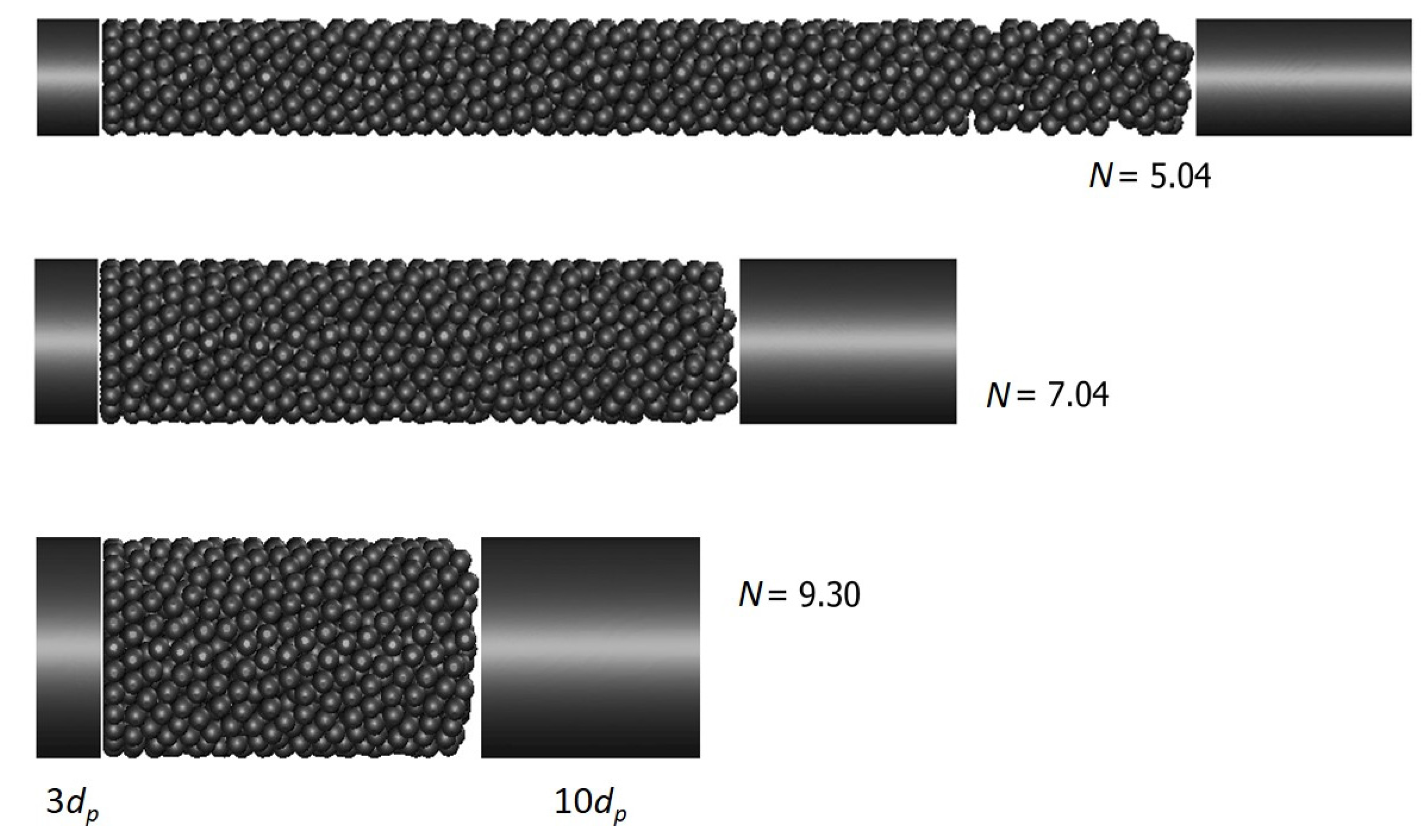
Eight beds of different N were generated, each packed with spherical particles of 0.0254 m diameter. The 3D random beds of spheres were produced using a modified soft-sphere collective rearrangement Monte Carlo algorithm [34]. The original algorithm was used along with a method to arrange the layer of spheres around the tube wall more realistically at the bottom of the tube [35]. Each bed consisted of three sections. The first was an empty section spanning 0.0762 m (3d_p) from the entrance of the bed, denoted as the “calming section.” The following section was the packed section, whose length is specified in

Table 1. Fixed bed configurations.

N	L/dp	No. Spheres	Bed Voidage
5.04	50.13	1000	0.442
5.45	40.12	1000	0.430
5.96	36.36	1080	0.429
6.40	31.97	1113	0.427
7.04	29.18	1200	0.431
7.44	26.63	1250	0.418
7.99	23.15	1250	0.414
9.30	17.01	1250	0.408

. The final section was another empty section, 0.254 m (10d_p) in length, used to mitigate backflow effects near the exit of the bed. The bulk void fractions in Table 1 were calculated using the center section of the bed, from 5d_p above the inlet to 3d_p below the outlet, to exclude end effects, except for N = 5.04, where a shorter length was used to avoid packing defects.

The model geometry is shown for three of the beds in Figure 1. These beds represent the smallest, largest and an intermediate value of N. Since only fluid transport mechanisms were to be simulated, only the fluid domain needed to be meshed. Tetrahedral cells characterized the fluid domain, and the control volume linear size was 0.00127 m, which corresponded to d_p/20. Boundary or prism layers extended from the particle and tube wall surfaces into the fluid and were 2.54 × 10⁻⁵ m thick. This gave mesh counts of 30.2–40.3 M cells depending on the value of N. Mesh refinement studies were carried out on a smaller test column with N = 3.96, using tetrahedral cells of sizes d_p/16.7 (0.00152 m), d_p/25 (0.001016 m) and d_p/33.3 (0.000763 m), which gave mesh counts from 4.2–30.0 M cells. Excellent agreement was observed for void fraction and interstitial velocity radial profiles for all mesh sizes, with average differences on the order of 1%–2%. Further mesh refinement tests were made using three prism layers on the tube surfaces, again with excellent agreement between profiles.

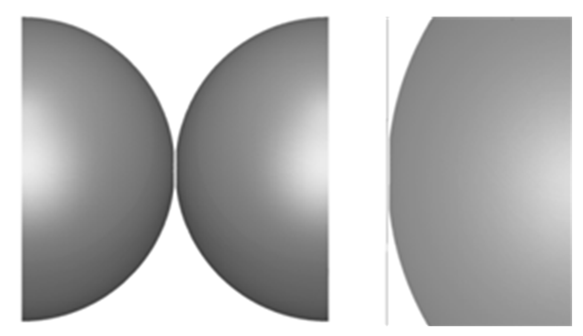
The contact points between spheres and between the spheres and the tube wall give very narrow “fillets” of fluid, which cause problems in meshing. Various methods have been compared to deal with this difficulty [36], and a local modification using the “caps” contact point approach [37] was selected as being suitable for flow problems with no heat transfer. In our implementation of this method, a small cylinder of height 5.13 × 10⁻⁴ m was aligned with its axis along the vector connecting the particle centers and centered at the contact point between the particles, then subtracted from each particle and replaced by a small amount of fluid. At the particle-wall contacts, a similar procedure was followed; this cylinder was 6.15 × 10⁻⁴ m in height, slightly larger because of the opposite curvature of the tube wall. The bed void fraction change from this modification to the geometry was less than 0.5%. The modifications are shown schematically in Figure 2.

2.4. Boundary Conditions

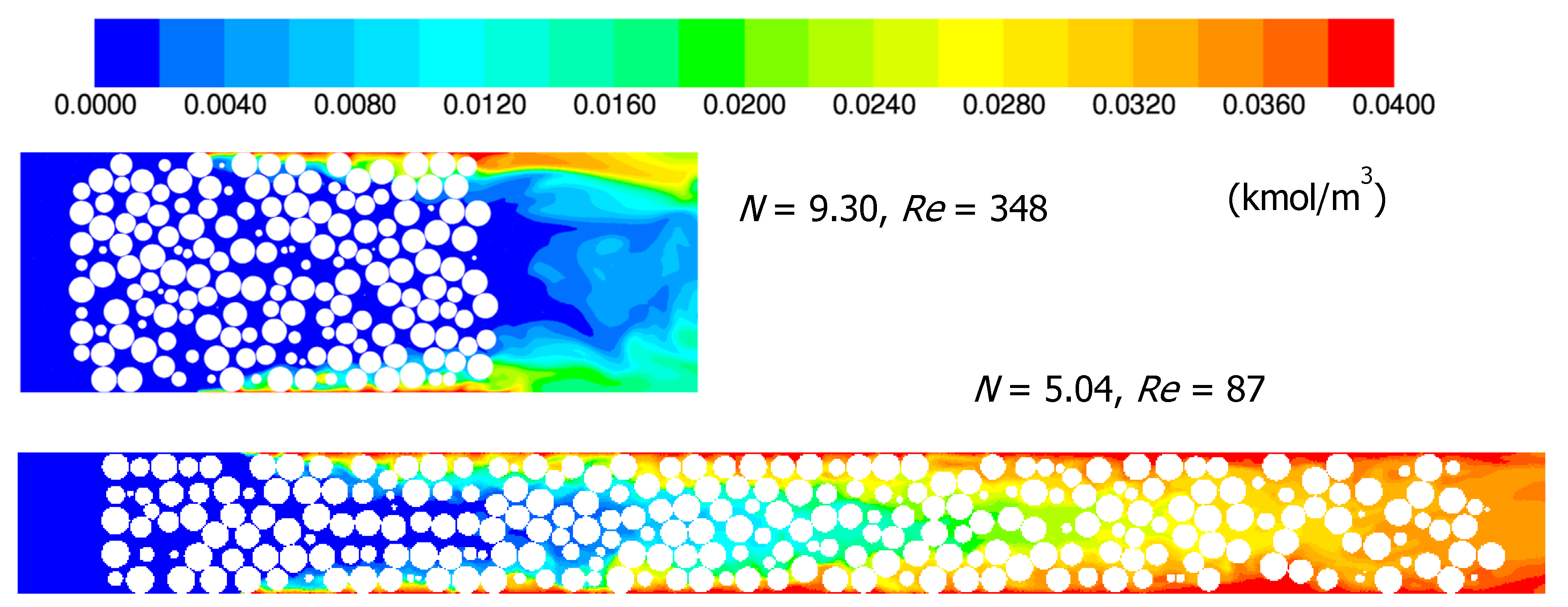
To obtain velocity profiles in the bed, a uniform velocity boundary condition was set normal to the inlet of the tube, for each of the four particle Reynolds numbers used in this study, namely Re = 87, 348, 696 and 870. For these flow rates, direct numerical simulation was used. Air was specified as the fluid in the bed, with constant properties for isothermal conditions (i.e., μ = 1.7894 × 10⁻⁵ kg/m/s, ρ = 1.225 kg/m³). A constant pressure condition was specified at the exit of the tube as atmospheric pressure. No-slip boundary conditions were assigned to the tube walls and particle surfaces.

The focus of this work was to model dispersion and more specifically near-wall effects in low-N beds, by simulating methane diffusion from a coated tube wall into flowing air. To avoid unrepresentative concentration profiles caused by developing flow, the first 5d_p axial length of the bed was uncoated to allow flow to become established. The coated section was implemented by setting the methane species mass fraction as unity on the tube walls.

2.5. Computational Aspects for Computational Fluid Dynamics (CFD)

The semi-implicit pressure-linked equations (SIMPLE) method for pressure-velocity coupling was chosen [33]. The least squares cells approach was selected for the gradient method. For spatial discretization, the first-order upwind scheme was chosen for pressure, momentum and species for the first 200–300 solution iterations, to take advantage of the stability properties. After iterations stabilized, the discretization was switched to the more accurate second-order upwind for the remainder of the solution.

Solution convergence was attained by ensuring that column pressure drop remained constant over at least 1000 iterations. For species transport, a monitor was added to a 2-mm isosurface at the end of the packed section to track methane concentration on each iteration step. Once the concentration was no longer monotonically increasing, the solution was deemed converged. A complete solution for a single case required approximately 15,000–20,000 iterations, with solution times averaging 1000 iteration steps per 12 h. All simulations were completed on a Dell R620 PowerEdge Server (Dell, Round Rock, TX, USA) running a Windows server 2008 R2 (Microsoft, Redmond, WA, USA) operating system. The server contained 2 Intel Xeon E5-2680 CPUs (Intel, Santa Clara, CA, USA), each with 8 cores, and 128 GB of Random-access memory (RAM).

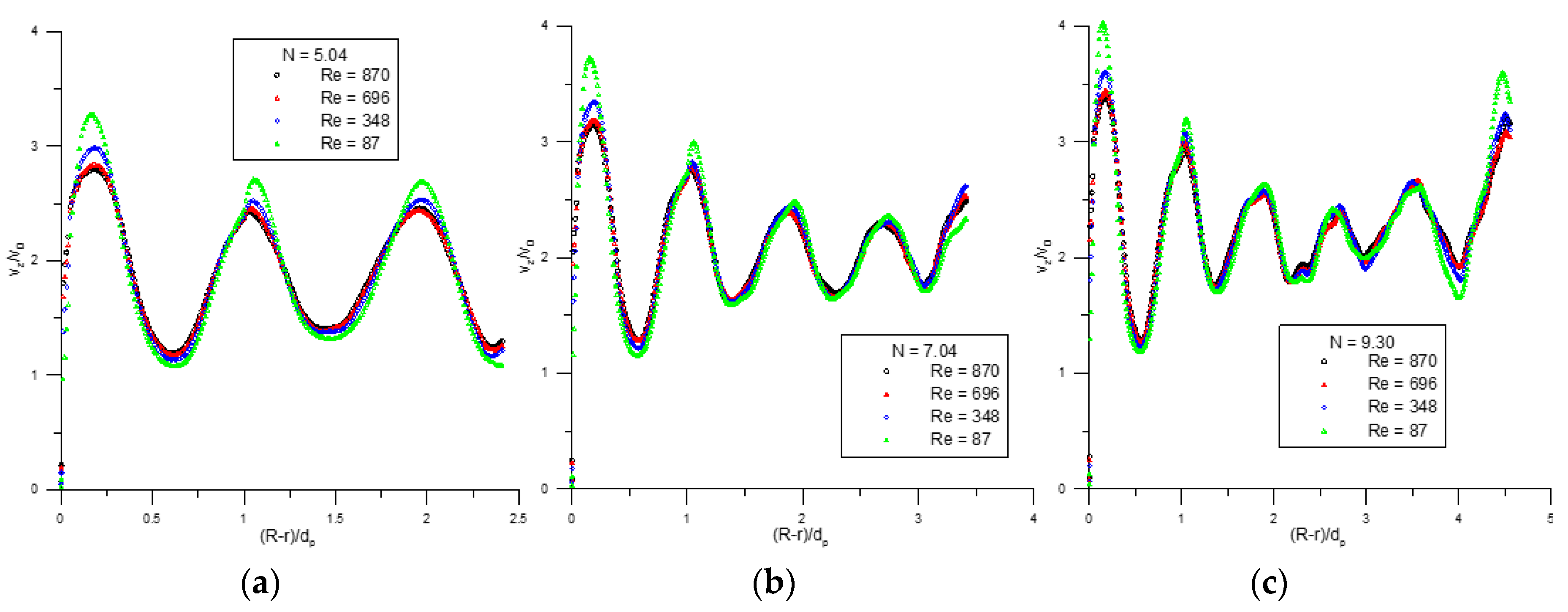
To obtain velocity and methane concentration profiles, cylindrical surfaces aligned axially with the bed were generated at various radial positions spanning the column diameter. The surfaces for axial velocity were clipped five particle diameters from the start of the bed packing and three particle diameters before the end of the packing, to prevent any end effects on the velocities. The resulting velocity profile was therefore averaged both axially and circumferentially. The surfaces for the methane concentrations were created similarly, with those surfaces clipped to 2 mm in height, at different axial positions, giving angularly-averaged methane concentration profiles across the diameter of the bed, at specified axial positions. Area-weighted averages were performed to collect both data sets for all runs.

2.6. Dispersion Models

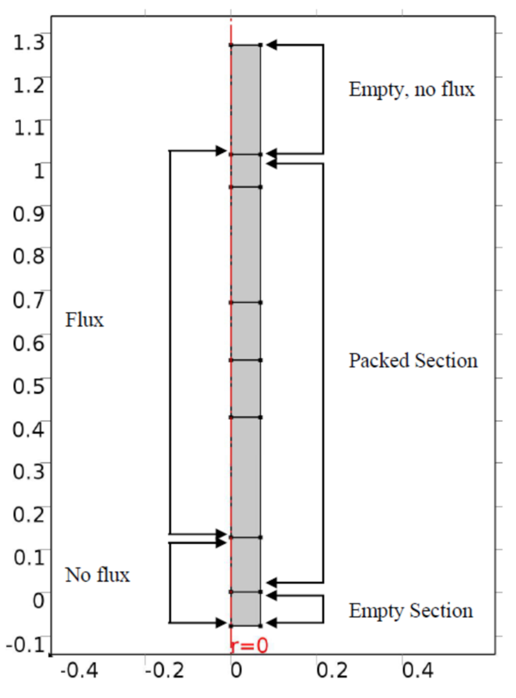
To obtain dispersion coefficients based on the CFD 3D resolved-particle simulation results, 2D effective medium dispersion models based on Equation (1) were used and their mass transfer parameters fitted to the CFD-generated radial profiles of methane concentration. The finite element commercial code COMSOL Multiphysics^® (COMSOL Inc., Stockholm, Sweden) was used. The two-dimensional domain was subdivided as shown in Figure 3 to reflect the corresponding sections in the 3D CFD model.

The radii of the beds simulated in COMSOL were the same as those in the CFD simulations. In Figure 3, the first two and the last sections of the bed represent those parts that were assigned a wall boundary condition of zero methane flux or zero methane concentration. These include the empty sections at the beginning and end of the tube. The “flux” section represents the portion of the 3D model that was assigned a non-zero wall mass fraction of methane. In the two-dimensional model, either a methane wall concentration or a non-zero wall methane flux condition is instead assigned, as detailed in the following subsections. The four horizontal internal boundaries were positioned at the z-values at which concentration radial profiles were extracted from the CFD simulations and were used as the dataset for fitting radial dispersion parameters. For each bed, the highest z-location was always three particle diameters below the top of the bed, to avoid exit effects, while sampling at the most developed profile location possible. The other three z-locations were originally approximately equidistant along the rest of the bed, but as results were analyzed, it was sometimes necessary to dispense with the lowest z-location and replace it with a location further down the bed, which corresponded to more developed concentration profiles.

The 2D domain was meshed with 32 layers of quadrilateral prisms on the tube wall surface, to capture the steep gradients there. The first layer thickness was 1/20 of the local element size, and a stretching factor of 1.3 was applied. The rest of the domain was meshed with triangular elements of sizes between 7.81 × 10⁻⁴ m and a maximum of 0.012 m. The coarse mesh sizes were used only in the bed center region, where the concentration profiles were relatively flat. Different mesh refinement settings were used within COMSOL^® to check for mesh-independence, which led to the given mesh sizes.

Optimization studies were conducted for each of the 2D models, coupled to the transport models within the COMSOL Multiphysics^® framework. The Levenberg-Marquardt least-squares optimization method was employed, which is commonly used for parameter fitting. The objective function was the sum of squares of deviations between the radial concentration profiles of methane, extracted from the CFD simulations at the four bed heights, and the corresponding methane radial concentration profiles from the 2D dispersion model under study. Each optimization was conducted for a given N and Re. The axial Péclet number remained constant at Pe_a = 2 in all runs. The study was complete when a minimization of the least-squares value of methane radial concentration deviations was achieved and an optimality tolerance (1 × 10⁻⁶) was met.

2.6.1. Model 1: Constant D_T

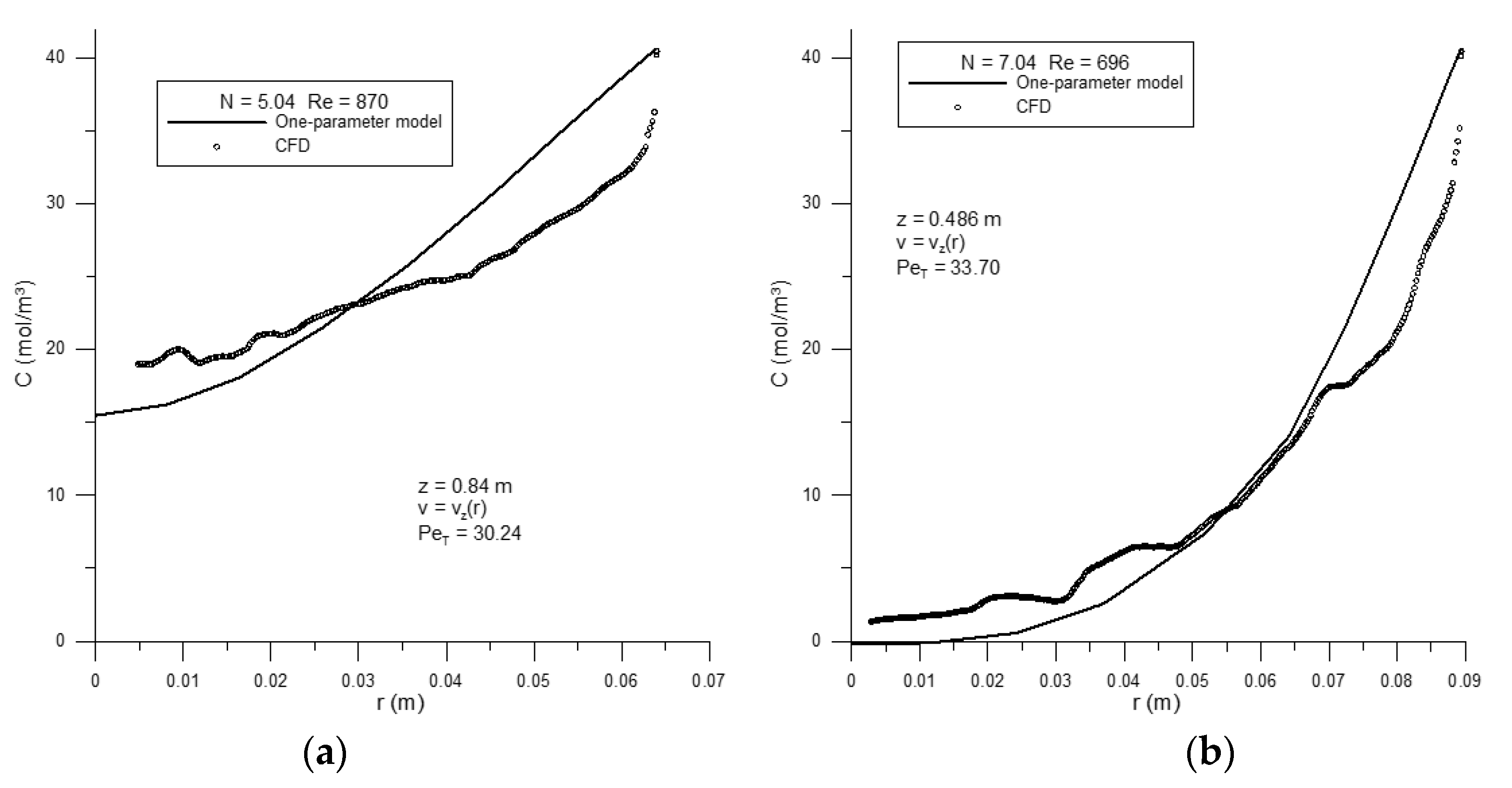
In this model, we tried to reproduce the developing radial concentration profile with a constant transverse dispersion coefficient and a radially-varying interstitial velocity:

$$v_z\left(r\right)\frac{\partial c_A}{\partial z}=\frac{{\overline{v}}_z{d}_p}{P{e}_L}\frac{{\partial }^2{c}_A}{\partial z^2}+\frac{{\overline{v}}_z{d}_p}{P{e}_T}\left(\frac{{\partial }^2{c}_A}{\partial r^2}+\frac{1}{r}\frac{\partial c_A}{\partial r}\right)$$

(11)

and at the coated tube wall r = R:

$$c_A=c_W$$

(12)

Here, $P{e}_L=\frac{{\overline{v}}_z{d}_p}{D_L}=2$ and $P{e}_T=\frac{{\overline{v}}_z{d}_p}{D_T}$. The only fitted parameter was $P{e}_T$.

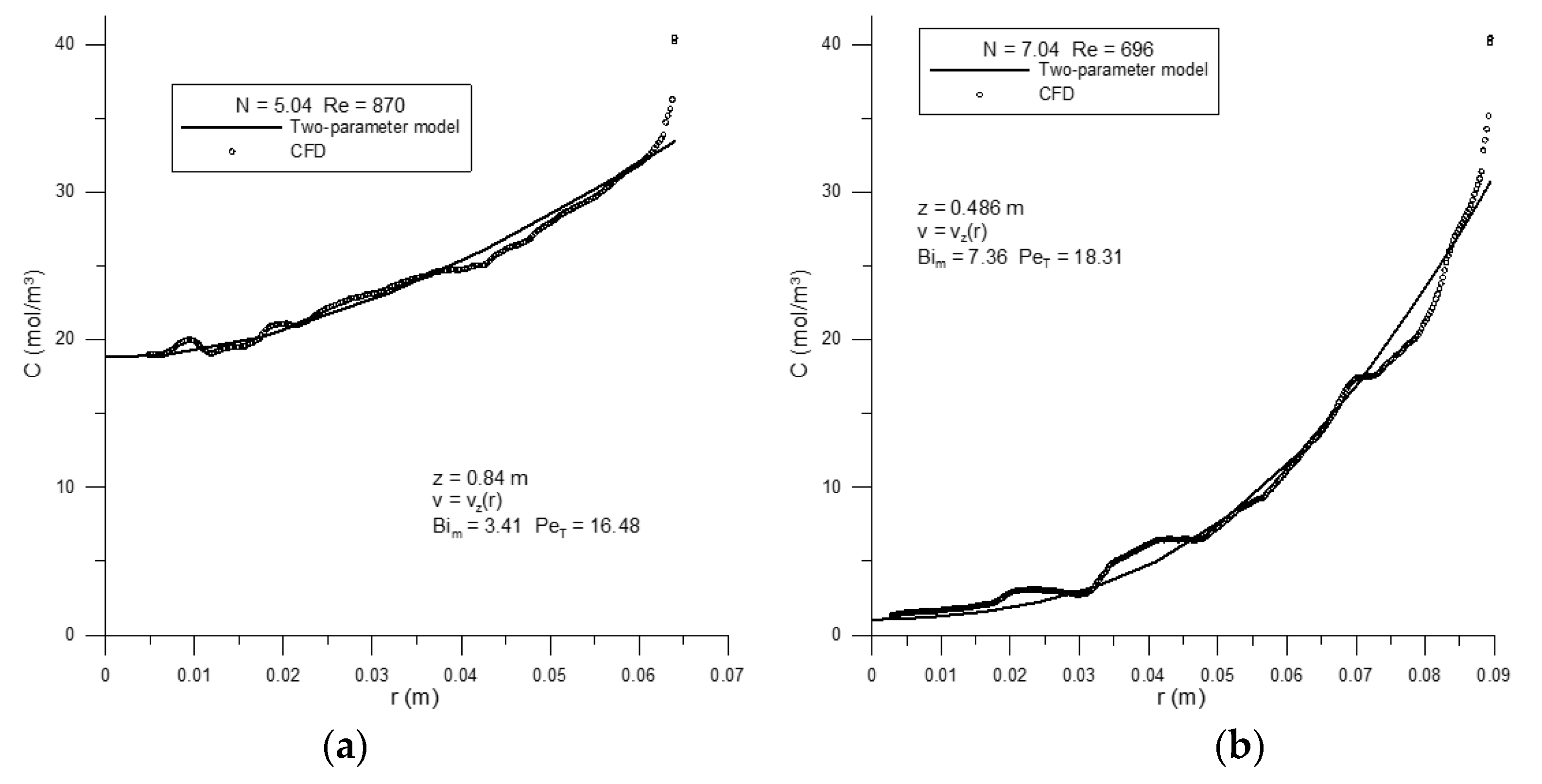
2.6.2. Model 2: Constant D_T and Wall k_m

In this model, we try to take account of the steep gradient near the tube wall by introducing a step change at the wall, governed by a wall mass transfer coefficient:

$$v_z\left(r\right)\frac{\partial c_A}{\partial z}=\frac{{\overline{v}}_z{d}_p}{P{e}_L}\frac{{\partial }^2{c}_A}{\partial z^2}+\frac{{\overline{v}}_z{d}_p}{P{e}_T}\left(\frac{{\partial }^2{c}_A}{\partial r^2}+\frac{1}{r}\frac{\partial c_A}{\partial r}\right)$$

(13)

and at the tube wall r = R:

$$-\frac{\partial c_A}{\partial r}=B{i}_m\frac{1}{R}\left(c_A-c_W\right)$$

(14)

Here, $P{e}_L=\frac{{\overline{v}}_z{d}_p}{D_L}$ (again equal to 2), $P{e}_T=\frac{{\overline{v}}_z{d}_p}{D_T}$ and $B{i}_m=\frac{k_{m}R}{D_T}$. The two fitted parameters were $P{e}_T$ and $B{i}_m$.

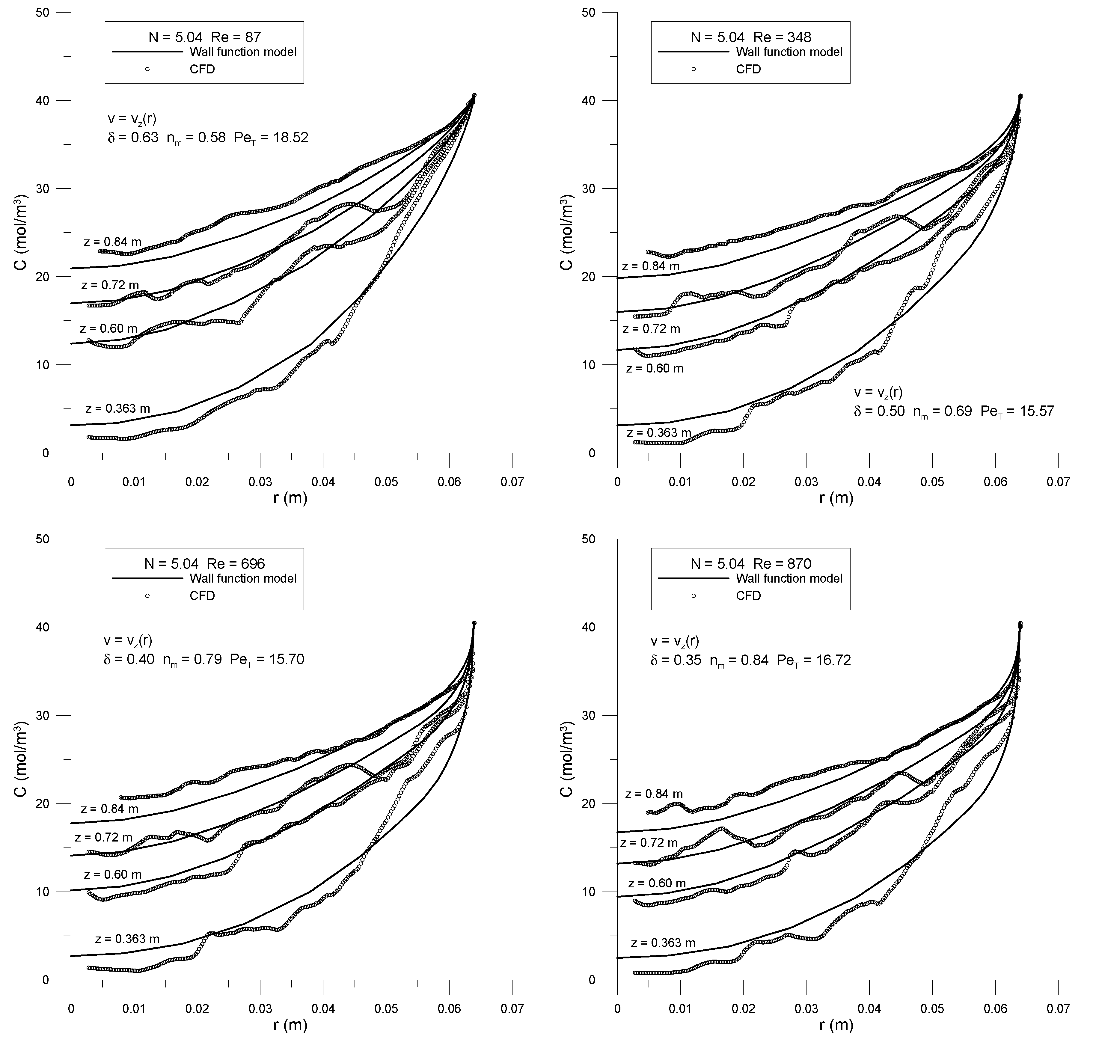
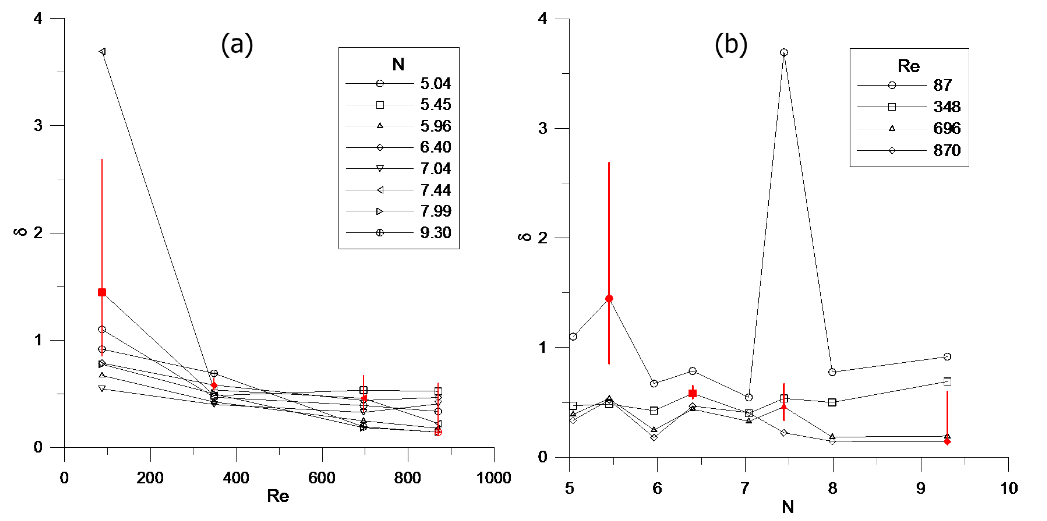
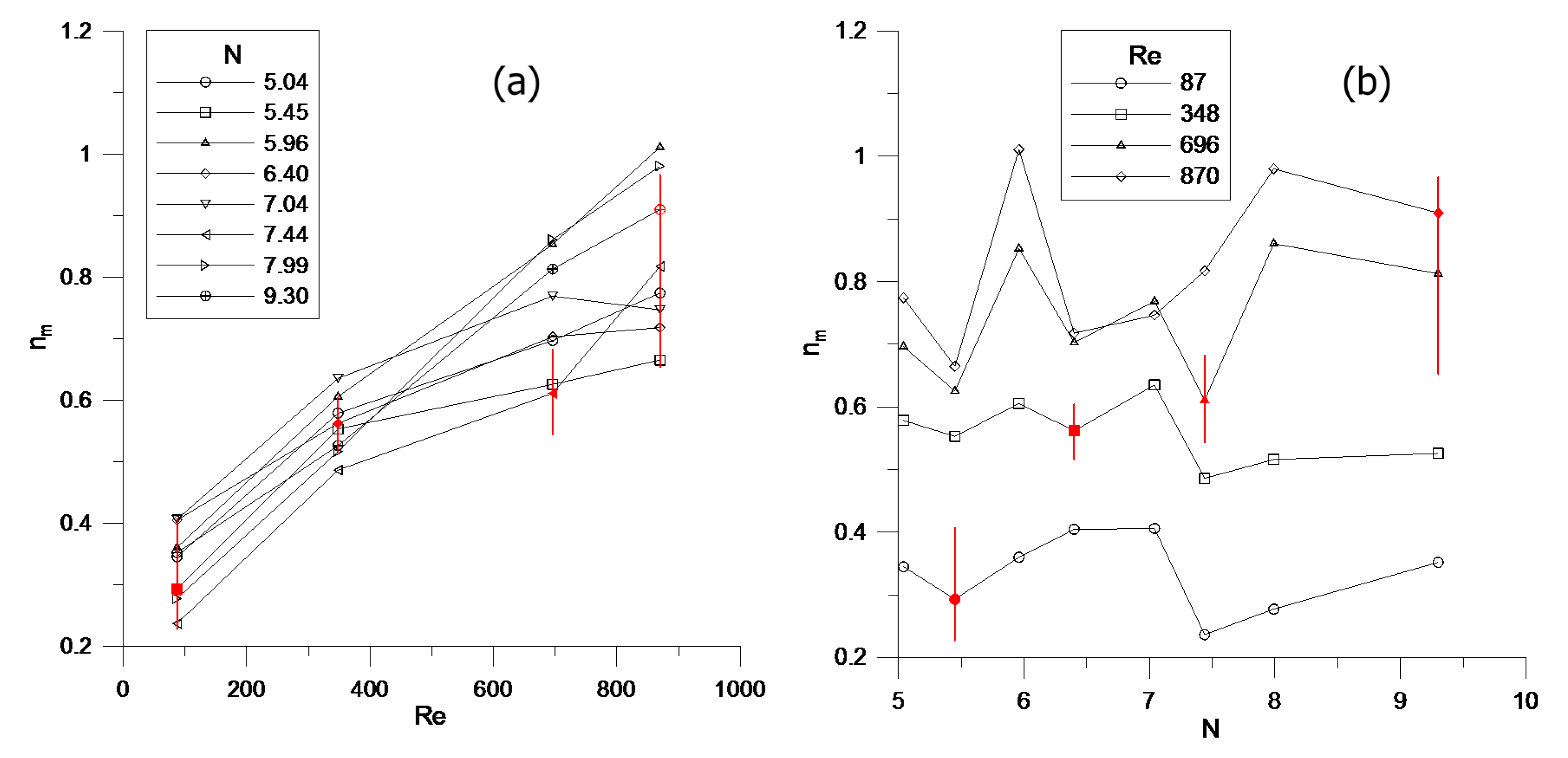
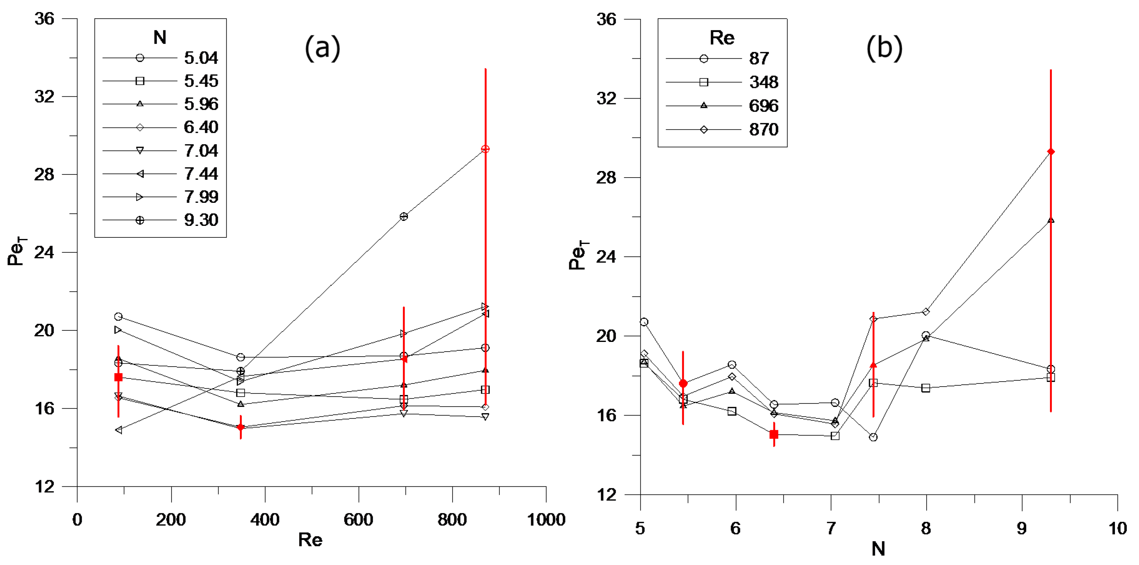
2.6.3. Model 3: Radially-Varying D_T

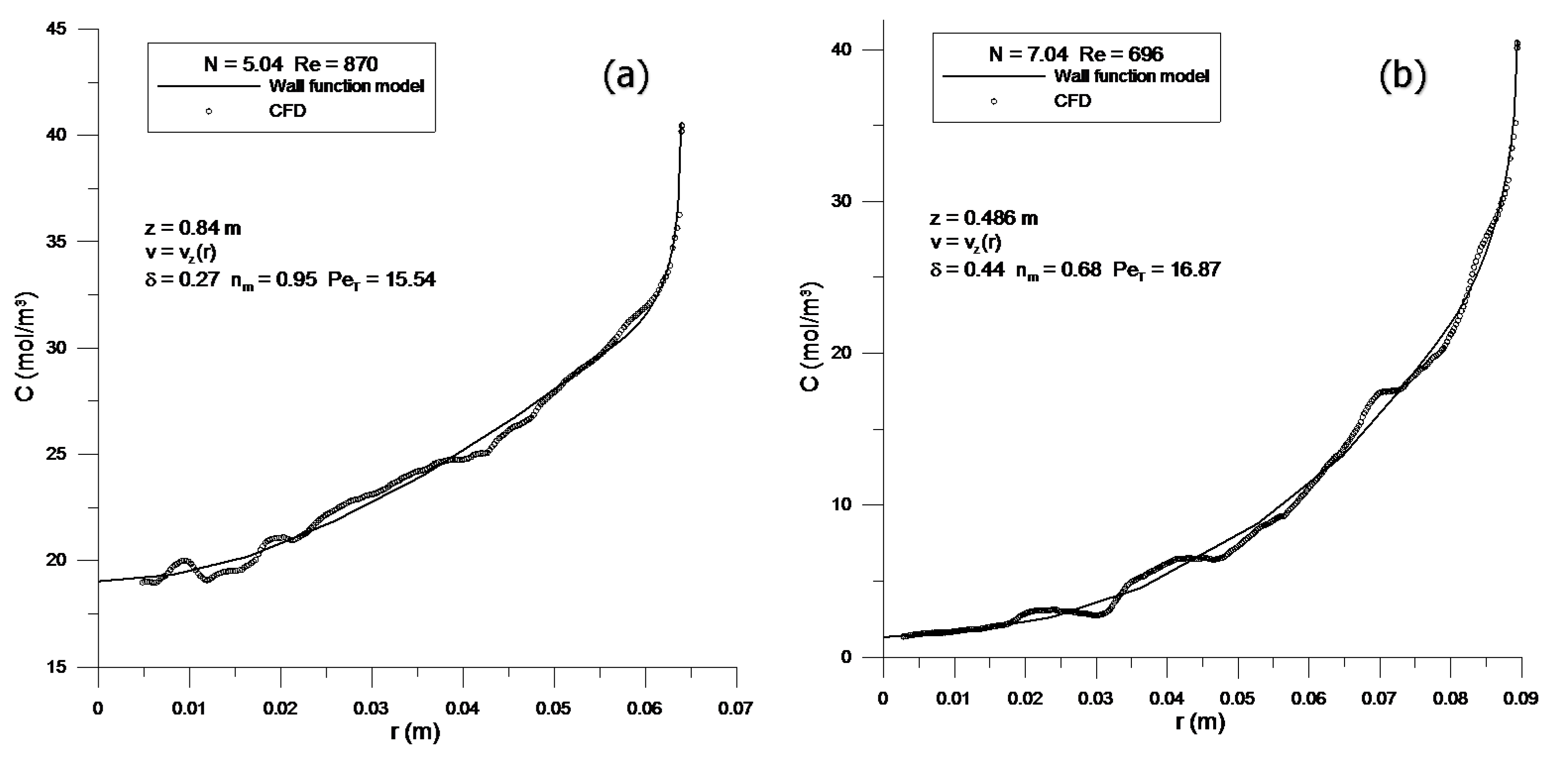
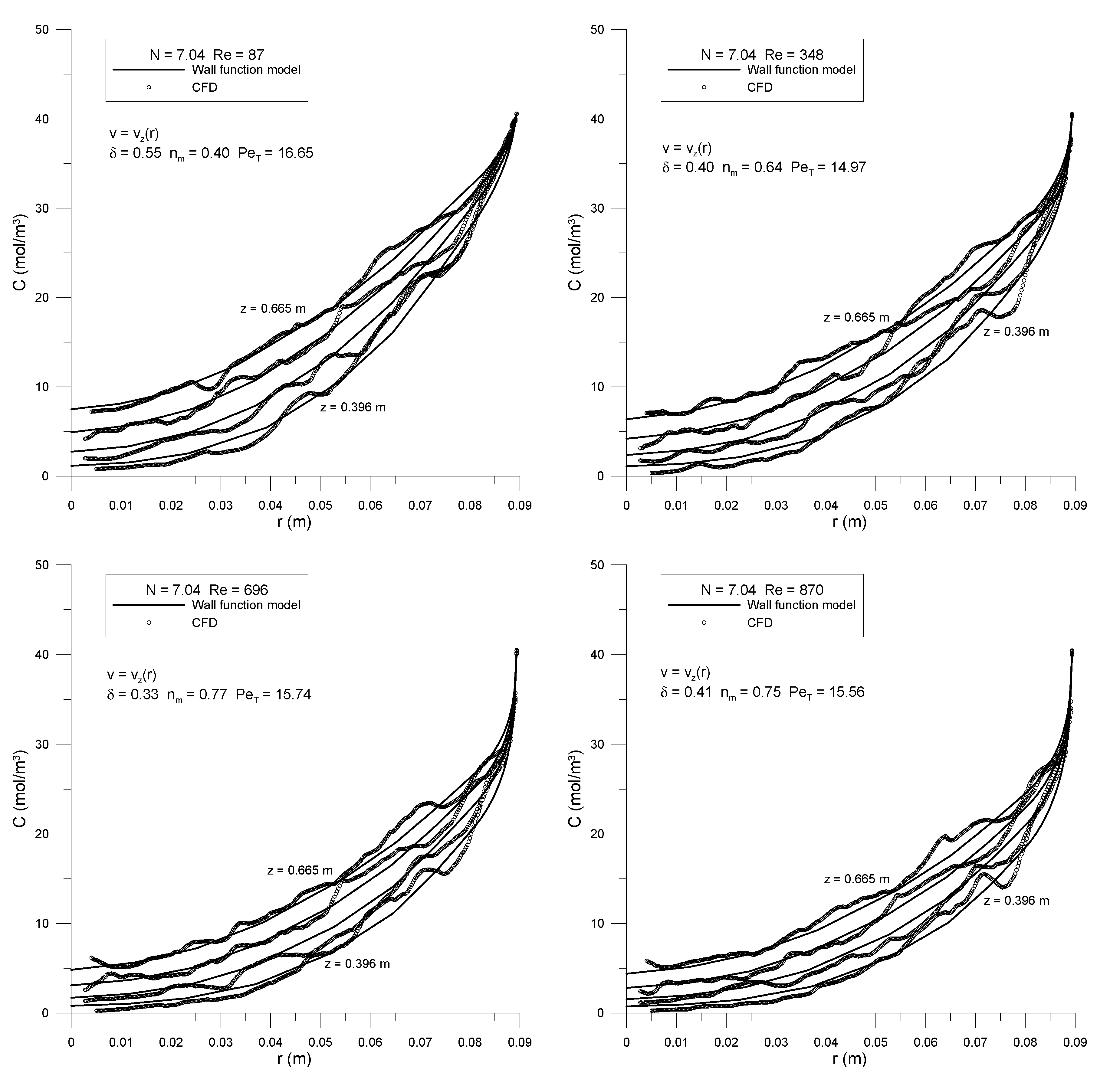
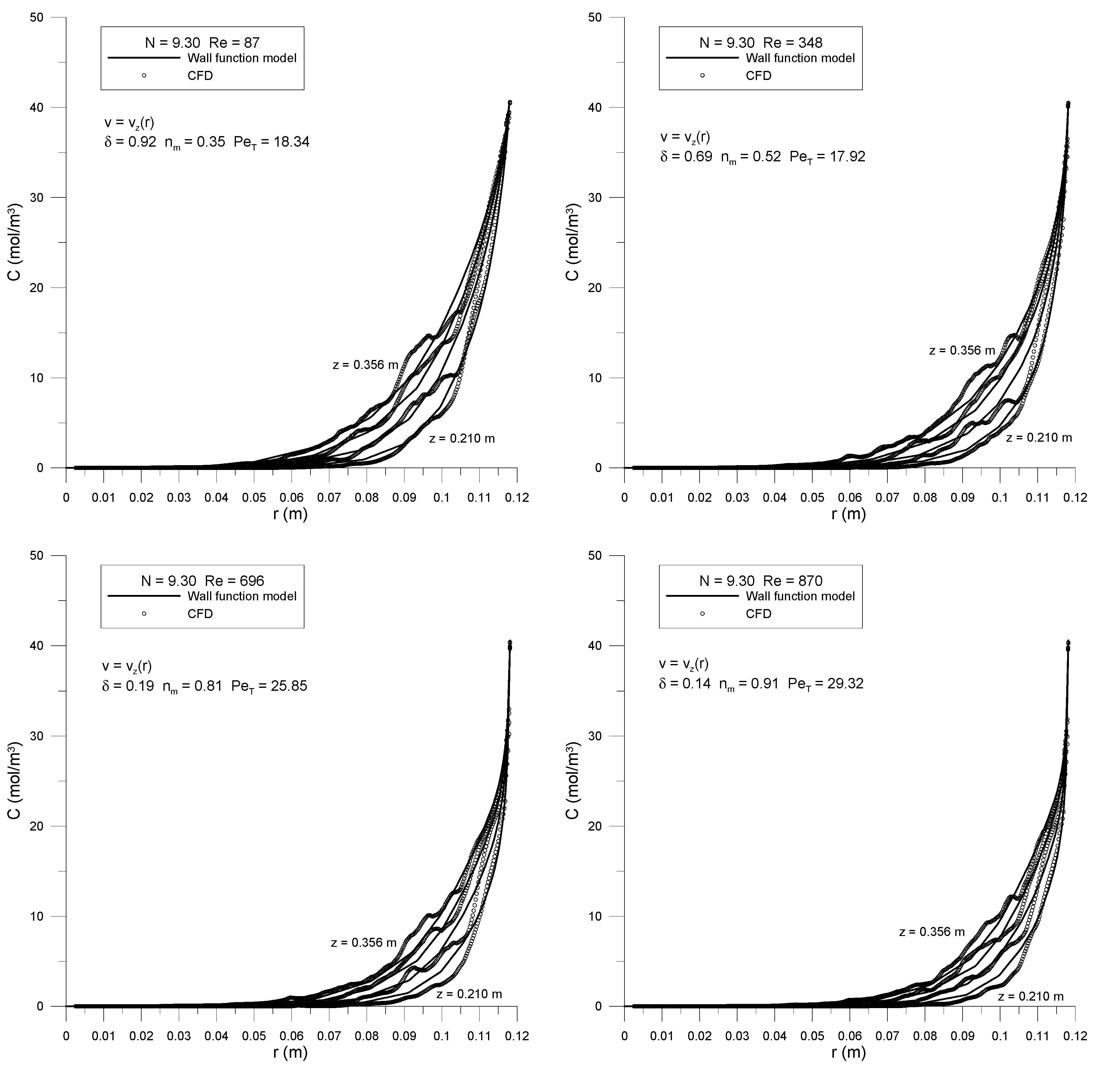
In this model, we use a simplified model for the transverse dispersion coefficient that decreases sharply near the tube wall to take account of the strong decrease in $D_T$ there, while being constant and neglecting any minor variations in the center of the packed bed:

$$v_z\left(r\right)\frac{\partial c_A}{\partial z}=\frac{{\overline{v}}_z{d}_p}{P{e}_L}\frac{{\partial }^2{c}_A}{\partial z^2}+\frac{1}{r}\frac{\partial }{\partial r}\left(r{D}_T\left(r\right)\frac{\partial c_A}{\partial r}\right)$$

(15)

and at the tube wall r = R:

$$c_A=c_W$$

(16)

Here, $P{e}_L=\frac{{\overline{v}}_z{d}_p}{D_L}=2$, and the simplified transverse dispersion coefficient is given by:

$$D_T\left(r\right)=D_m+\frac{{\overline{v}}_z{d}_p}{P{e}_T}f\left(R-r\right)$$

(17)

where:

$$f\left(R-r\right)=\{\begin{array}{cc}{\left[\frac{\left(R-r\right)}{\delta d_p}\right]}^{n_m}\hfill & 0<R-r \le \mathrm{ô}{d}_p\hfill \\ 1\hfill & \mathrm{ô}{d}_p<R-r \le R\hfill \end{array}$$

(18)

which is based on a mixing length model [31] and re-written following Winterberg et al. [32] with some differences. The three fitted parameters were $P{e}_T$, $\delta$ and $n_m$.

The original version of the model [32] was developed to include thermal conductivity and was therefore based on superficial velocity in both the differential equation and the equations for radial variation in the parameters, which used the bed-center value obtained by numerical solution of the Brinkman–Forchheimer–Darcy (BFD) differential equation. In our implementation of the model, the interstitial velocity is used for consistency with Model 1 and Model 2, and the bed center velocity is replaced by the bed-average interstitial velocity, obtained from the CFD velocity profiles, to avoid having to solve the BFD equation. Parameter δ gives the thickness of the region next to the tube wall (in d_p) over which the dispersion coefficient rapidly decreases; n_m controls the shape of the decreasing function; while Pe_T represents the constant bed-center transverse dispersion.

3. Results and Discussion

Validation of the 3D CFD model was made against available experimental data in the literature. Figure 4a shows an example comparing void fractions from the CFD model as a function of radial coordinate to data from Giese et al. [38], for the case N = 9.30. The computed void fractions agree very well with the experimental ones, especially near the tube wall where the strong decrease occurs. The oscillatory nature of the void fraction in a bed of spheres is also well captured, with the locations and magnitudes of the peaks and troughs in the profile in good agreement. Only at the bed center, where the sampling isosurfaces become small, some differences were seen, which is typical in fixed beds. Figure 4b shows comparisons of the normalized superficial velocity profile obtained in [38] by laser-Doppler anemometry on a single plane to the bed-average normalized superficial velocities from CFD obtained by multiplying the interstitial velocity by the void fraction at each radial position and dividing by the inlet velocity. Detailed agreement is less good than for the bed structure, but the major features are reproduced to an acceptable degree. The sharp peak near the wall is predicted by CFD close to that seen in the experimental data, while the locations of maxima and minima in the velocity are in good agreement. Magnitudes of the peaks are somewhat under-predicted, and some deviation is seen at the bed center, which is usual in such studies. The differences between CFD and experiment could be attributed to the sampling of a single plane in the experiments versus averaged velocities over most of the packed bed length in the CFD simulations.

3.1. 3D Computational Fluid Dynamics (CFD) Model

The images below in Figure 5 show contour plots of the concentration of methane taken from a center plane of the two beds, N = 5.04 and N = 9.30, for two selected values of particle Reynolds number Re, to illustrate the developing concentration fields obtained from the CFD simulations.

In the longer, narrower N = 5.04 tube, the full development of the concentration field can be seen. The local irregular penetration of the methane into the bed is evident, caused by the motion of the fluid between the wall particles. Regions of lower concentration near the wall can be seen caused by missing wall particles, which allow greater access of the fluid to the wall region. On average, however, a regular development is clearly seen. For the N = 9.30 tube, which due to computational constraints was necessarily shorter, the methane has only developed 2–3 particle diameters into the bed, and a large core of fluid free of the wall species persists the entire length of the bed. On exiting the bed, the fluid flow pattern exhibits regions of re-circulation and lateral motion, which are reflected in the irregular regions of high and low concentration.

Figure 6 displays the velocity profiles of three selected beds at all particle Reynolds numbers. Each plot contains axial interstitial velocity normalized by the superficial velocity set at the bed entrance. With each bed diameter, the velocity at the lowest Reynolds number (Re = 87) peaks higher than for the other three velocity profiles, which are essentially coincident. This is due to viscous forces in the flow becoming more significant compared to inertial forces at low Re. The velocities approach zero towards the tube wall, owing to the no-slip boundary condition. This low-velocity region is the reason for the separation of the diffusion-dominated wall boundary layer from the dispersion-dominated flow in the rest of the bed. From a comparison of the void fraction profiles, higher axial velocities appear in areas of highest radial void fraction (i.e., low velocities in areas of low bed porosity, except in the near-wall vicinity). Near the wall, when the void fraction is close to unity, a channeling effect occurs, in which flow becomes axial. In this region, resistance to radial mixing is strong, giving a decrease in transverse dispersion.

3.2. One-Parameter Dispersion Model

Typical results for fits of the one-parameter model to single bed depth data are shown in Figure 7, for two values of N and Re. All combinations of N and Re were fitted and gave the same qualitative results. The one-parameter model is clearly unable to describe the developing concentration profiles, although literature results have indicated that it is sufficient for well-developed profiles. In this model, the concentration is forced to take the value c_w at the tube wall. This constrains the shape of the profile, which can reproduce neither the flatter profile region in the bed center, nor the steep increase near the tube wall. It was also found that there was a strong dependence of Pe_T on bed depth, L, and poor fits were obtained if the model was fit to all four bed depths simultaneously.

The dependence of Pe_T (and hence, D_T) on L can be understood by considering that in fact the dispersion must vary with radial position, due to the change in void fraction and velocity close to the tube wall. The use of a constant D_T means that this variation is being represented by an average value, and the value of this average depends on which parts of the radial concentration profile contribute most heavily to the least-squares objective function. That is, a profile that is just starting to develop will be influenced more by the lower values of D_T near the wall, than will a profile that is developed across the whole radius, which will be influenced also by higher dispersion values in the bed center.

3.3. Two-Parameter Dispersion Model

From the one-parameter model results, the next idea is that since most of the change in D_T is anticipated to take place very close to the tube wall, it may be possible to account for it by introducing a wall mass transfer coefficient k_m and retaining the constant D_T. This essentially idealizes the extra resistance to mass transfer in the region of the tube wall, to a resistance located at the tube wall. Typical results are shown in Figure 8. In general, the fitted model predicts methane concentration away from the tube wall with both good qualitative and quantitative agreement. The model is unable to reproduce the increase in concentration in the region of the tube wall.

The wall concentration is better predicted for higher N, lower Re and lower bed depth combinations, as these correspond to situations in which the difference between the near-wall region and the bed center is reduced. In beds of lower N and higher Re and higher bed depth (e.g., N = 5.04, Re = 870), small gradients in methane concentration characterize the radial concentration profiles. In these cases, enough methane has dispersed laterally from the wall and been transported axially up the bed that a smaller drop in concentration from the wall value is seen at the longer bed depth.

The fitted values of Pe_T were somewhat higher than would be expected from literature studies of fully-developed profiles without wall effects [3,4]. This observation corresponds to lower values of the transverse dispersion coefficient. The values of Bi_m for the wall mass transfer coefficient were also quite high, which may be due to the same low D_T. A possible explanation is that the methane dispersion is controlled by slow diffusion through the wall boundary layer and then dispersed at a reduced rate of convective-dispersion at the interface between the diffusive-dispersion and convective-dispersion layers. Previous literature has shown also that 2D models predict higher dispersion coefficients to their 3D counterparts due to higher intercellular fluid motion in the lateral direction [30]. These coupled effects may serve as an explanation for the lower than expected dispersion coefficient values found in this research.

It appears that the mechanism of dispersion should be quantified by at least three types: slow, diffusive-dispersion in the tube wall boundary layer; then, an increasing rate of dispersion at the diffusive-dispersion and convective-dispersion interface and toward the tube center and, finally, a fully convective dispersion at the tube center. The use of the two-parameter model shown here reduces this mechanism to two parts: that of constant radial dispersion from the tube center and up to the wall, at which point a jump in concentration is implemented by the mass transfer coefficient. This limits the physical realization of the various dispersion mechanisms in the bed.

A separate study was conducted using N = 5.04, 6.40 and 9.3 in which the velocity profile was taken constant. The dispersion coefficients predicted with a constant velocity profile were 10%–20% higher than those obtained with a variable velocity. The unidirectional, constant velocity profile includes a nonzero velocity up to the wall, so that the axial convection of mass is higher in the near-wall region, which would reduce transverse mass transfer. To compensate for this, the transverse dispersion coefficient is increased in the fitting process, which would result in lower Pe_T values. The combination of fitting to developing profiles rather than fully-developed ones and using a radially-varying velocity profile rather than plug flow may account for the decreased transverse dispersion coefficients found for this model.

3.4. Three-Parameter Dispersion Model

The results from the two-parameter model suggested that more detail was required to represent the effects of the tube wall on D_T. In the three-parameter model, D_T varies with the radial coordinate controlled by three parameters, $P{e}_T$, $\delta$ and $n_m$. A typical profile of D_T(r) is shown in Figure 9.

The general form of the D_T(r) profile is a constant through most of the bed, followed by a steep decrease in the vicinity of the wall, so that it may be termed a wall-function model. The magnitude of the bed center dispersion coefficient value is controlled by Pe_T, which changes in inverse proportion to D_T. The width of the region over which D_T decreases is given by δ as a fraction of a particle diameter, so that in the example provided in Figure 9, the near-wall region is of thickness 0.32d_p. The form of the decrease is governed by the parameter n_m, which results in a convex function as shown for values less than unity and a concave function for values greater than unity. The convex function gives a decrease, which becomes steeper as the radial coordinate approaches the tube wall, as opposed to the concave function, which is steepest at the initial point of transition from a constant to a variable D_T. The profiles in the present study were always represented better with the convex shape with n_m < 1, a different result than that found for heat transfer in [32], where n_m ≈ 2.

The results of fitting the radial methane concentration profiles one depth at a time using the three-parameter model gave a great improvement, as shown in Figure 10 for the same two cases that were presented previously in Figure 7 and Figure 8, for ease of comparison. The fitted profiles are able to follow both the flat regions in the bed center, as well as the steep gradients very close to the tube wall. Again, similar results were seen for all eight values of N, four values of Re and four bed depths. The only aspects of the profiles that were not reproduced were the slight oscillations, familiar in heat transfer studies, which measure radial temperature profiles and which are attributable to the discrete nature of the ordered layers of the spheres adjacent to the wall. To reproduce these oscillations or “humps” would require a function for the radial dispersion parameter that mirrored the particle level changes. This is a level of detail that may not be worth pursuing. The estimates of all three parameters did change, often quite drastically, with bed depth, but no systematic trends in the changes could be found. The results of the individual bed depth fitting show that the fit was improved by the inclusion of a third parameter, which allowed the inclusion of a more nuanced treatment of the radial variation of the dispersion coefficient.

The next step was to see if the model could fit all bed depths simultaneously and whether depth-averaged parameter values would give acceptable fits. Results are presented in Figure 11, Figure 12 and Figure 13. Figure 11 shows relatively well-developed methane radial concentration profiles for the N = 5.04 case. The methane has dispersed from the tube wall across the entire tube radius, so that the radial concentration gradients are relatively small, and at the longest bed depths, the profiles are quite flat. At all four values of Re, the model slightly over-predicts the concentrations in the bed center at the lowest bed depth and under-predicts the profile in the bed center at the highest bed depth. The two profiles at the middle depths are in good agreement, but even there, a slight trend can be seen suggesting that the predicted profiles show lower spread with bed depth than the CFD-generated ones. This disagreement occurs only for the profiles for N = 5.04; even for N = 5.45 and N = 5.96, the axial spread of CFD profiles and fitted profiles is in good agreement (see Figures S1–S5 in the Supplementary Material). Near the tube wall, the profiles all come closer together, as the boundary condition forces c_A −> c_w for all. As for the individual bed depths, the steeper near-wall gradients are well captured. The fits to the set of four bed depths are reasonable with a single set of parameters.

Steeper radial concentration profiles are shown in Figure 12, for N = 7.04, in which the methane dispersing from the tube wall has only just reached the tube center at r = 0. The spread in the profiles in the center of the bed is much less than in the N = 5.04 case and is quite well captured by the model. Again, the profiles near the tube wall are close together, and the model does well in reproducing them. In particular, the increasingly steep gradient of concentration adjacent to the tube wall with increasing Re is followed, even with the fairly simple treatment of decreasing radial dispersion used in the model. In all cases, there is clearly considerable local variation in the shapes and details of each profile, but the overall trend, magnitudes and gradients of the profiles are fitted well by the three-parameter wall function model.

In Figure 13, the fits for the non-developed profiles of the highest tube-to-particle diameter ratio N = 9.30 case are presented. The CFD-generated radial methane concentration profiles here are flat in the center of the tube, as the methane has not been able to disperse across the full tube radius. This is due to the wider tube, which increases the distance for material to disperse, and also the shorter tube length, which was constrained by the computational restrictions on the total number of particles that could be simulated. This shape of profile, which combines extremely sharp gradients near the tube wall and flat profiles with no gradients at all in the tube center, provides a severe test of the wall-function model’s ability to reproduce a profile in the early stages of development. As can again be seen, the model is in excellent agreement with the CFD profiles over the entire radius, even as the gradients increase with higher Re. The spread of the four profiles with bed depth is less in this case than for the other two shown in Figure 11 and Figure 12, and even that reduction is followed by the model.

The results shown for the three N values in Figure 11, Figure 12 and Figure 13, as well as the five other N values presented in the Supplementary Material confirm that a model that incorporates the reduction in transverse dispersion over a region near the tube wall can fit a wide variety of profiles over the ranges of N and Re studied. This type of model improves on the representation of the complex radial variation of transverse dispersion by distributing a decrease over a finite region, instead of neglecting it or idealizing it to a point. Even a simple mixing-length approach is sufficient to accommodate both sharp and flat gradients, in profiles that range from ones starting to develop to others that are almost fully developed. The greatly improved ability of this three-parameter model to fit these profiles, compared to the one-parameter and two-parameter models, counter balances the disadvantage of having to estimate and correlate an extra parameter.

Having demonstrated that the three-parameter model can provide excellent agreement with CFD-generated developing radial concentration profiles, the next step is to determine whether reasonable correlations for the three parameters can be obtained. The parameters are presented in Figure 14, Figure 15 and Figure 16 as functions of the main variables, N and Re. In each case, there is a reasonable amount of variation in the parameter, as well as one or two points that represent outliers from the main trends. The runs corresponding to these outliers were re-examined for anomalies, but in each case, the results were confirmed. The fitted values of the parameters in these cases may be due to the randomly- generated bed structures, leading to the occasional anomalous feature in the concentration profiles.

From Figure 14, the parameter δ, which represents the width of the near-wall region scaled by particle diameter, can be seen to have a weak dependence on N and to decrease with increasing Re. These trends may be explained by considering that for any N, the arrangement of spheres next to the tube wall is similar, as has been suggested by radial void fraction profiles [37] and velocity profiles (Figure 6 above), which almost (with the exception of Re = 87) fall onto a single curve when properly scaled. As Re increases, also, the convective contribution to transverse dispersion will increase, and the diffusive layer next to the tube wall will be expected to decrease in thickness.

The shape of the decrease in D_T is represented by the parameter n_m, which is seen in Figure 15 to have a strong dependence on Re, increasing from approximately 0.2 up to nearly 1.0 over the range studied here. It is possible that at higher Re, the shape of the function may change and the value may approach 2.0, as found for heat transfer by Winterberg et al. [32]. The reason may be that at higher flow rates, the differences between the two approaches in use of the velocity profile may become less important. The parameter n_m may be taken as independent of N, as shown in Figure 15b.

Finally, the parameter Pe_T as shown in Figure 16 is independent of Re except that it is possibly a little higher for Re = 87. This is consistent with values of transverse dispersion for gases [1,2,3,4] in which the convective contribution dominates and the asymptotic value of Pe_T is reached for Re > 100–200, approximately. Pe_T depends only weakly on N, showing a slight increase at higher N values. The range for Pe_T is 16–20, which is again a little higher than for the cases in which only fully-developed profiles are considered, without wall effects.

For a chosen set of runs, the variance inherent in the CFD data (no replicates in computer simulation) was estimated by forming the sum of squares of the deviations of the CFD points around the fitted curve and dividing by the number of degrees of freedom. Two alternative cases were made, one by adding the square root of this variance (or a sample estimate of standard deviation) to each point of the original CFD data and one by subtracting the standard deviation from each point. The model was then re-fitted to each of the two new datasets, and the range of parameter estimates obtained was taken as an indication of the uncertainty in the parameter estimates. These ranges were then plotted in Figure 13, Figure 14, Figure 15 and Figure 16 as red, vertical lines, and the original CFD data points were also plotted in red so that they would be clearly visible. Note that these “confidence intervals” are not centered on the original data, which is normal for nonlinear parameter estimation. The uncertainty ranges depend on both N and Re and can vary considerably in magnitude. Despite that, the observed trends in the parameters are seen to be significant even in comparison to the uncertainties involved.

4. Conclusions

Literature studies [1,2,3,4] have shown that in the absence of wall effects, i.e., for well-developed concentration profiles, radial dispersion in a packed tube can be described satisfactorily through the use of a single transverse dispersion coefficient. The present study has shown that to describe the development of radial concentration profiles in the presence of wall effects, neither a one-parameter model, nor a two-parameter model that incorporates a wall mass transfer coefficient are adequate. It is necessary to allow for a region of primarily diffusive mass transfer adjacent to the tube wall, a transition region where both diffusive and convective transfer are important, and the bed center region, which is dominated by convective dispersion. Our work has shown that a three-parameter model based on a mixing length concept [31,32] in which the transverse dispersion coefficient varies with radial position can represent the developing profiles even with a relatively simple functional dependence on tube radius. Further work should investigate the development of an equation for the velocity profile in the bed that can be used in engineering (as opposed to CFD) models and the provision of quantitative and reliable correlations for the three model parameters.

References

1. Gunn, D.J. Theory of axial and radial dispersion in packed beds. Trans. Inst. Chem. Eng. Chem. Eng. 1969, 47, T351–T359. [Google Scholar]
2. Gunn, D.J. Axial and radial dispersion in fixed beds. Chem. Eng. Sci. 1987, 42, 363–373. [Google Scholar] [CrossRef]
3. Delgado, J.M.P.Q. A critical review of dispersion in packed beds. Heat Mass Transf. 2006, 42, 279–310. [Google Scholar] [CrossRef]
4. Delgado, J.M.P.Q. Longitudinal and transverse dispersion in porous media. Chem. Eng. Res. Des. 2007, 85, 1245–1252. [Google Scholar] [CrossRef]
5. Bernard, R.A.; Wilhelm, R.H. Turbulent diffusion in fixed beds of packed solids. Chem. Eng. Prog. 1950, 46, 233–244. [Google Scholar]
6. Fahien, R.W.; Smith, J.M. Mass transfer in packed beds. AIChE J. 1955, 1, 28–37. [Google Scholar] [CrossRef]
7. Hiby, J.W. Longitudinal and transverse mixing during single-phase flow through granular beds. Interact. Fluid. Part. 1962, 312–325. [Google Scholar]
8. Gunn, D.J.; Pryce, C. Dispersion in packed beds. Trans. Inst. Chem. Eng. 1969, 47, T341–T350. [Google Scholar]
9. Han, N.-W.; Bhakta, J.; Carbonell, R. Longitudinal and lateral dispersion in packed beds: Effect of column length and particle size distribution. AIChE J. 1985, 31, 277–287. [Google Scholar] [CrossRef]
10. Schertz, W.W.; Bischoff, K.B. Thermal and material transport in nonisothermal packed beds. AIChE J. 1969, 15, 597–604. [Google Scholar] [CrossRef]
11. Foumeny, E.A.; Chowdhury, M.A.; McGreavy, C.; Castro, J.A.A. Estimation of dispersion coefficients in packed beds. Chem. Eng. Technol. 1992, 15, 168–181. [Google Scholar] [CrossRef]
12. Yagi, S.; Wakao, N. Heat and mass transfer from wall to fluid in packed beds. AIChE J. 1959, 5, 79–85. [Google Scholar] [CrossRef]
13. Kunii, D.; Suzuki, M. Heat and mass transfer from wall surface to packed beds. J. Fac. Eng. Univ. Tokyo B 1969, 30, 1–15. [Google Scholar]
14. Storck, A.; Coeuret, F. Mass transfer between a flowing liquid and a wall or an immersed surface in fixed and fluidised beds. Chem. Eng. J. 1980, 20, 149–156. [Google Scholar] [CrossRef]
15. Dixon, A.G.; DiCostanzo, M.A.; Soucy, B.A. Fluid-phase radial transport in packed beds of low tube-to-particle diameter ratio. Int. J. Heat Mass Transf. 1984, 27, 1701–1713. [Google Scholar] [CrossRef]
16. Colledge, R.A.; Paterson, W.R. Heat transfer at the wall of a packed bed: A j-factor analogy established. In Proceedings of the 11th Annual Research Meeting, Bath, UK, 9–10 April 1984; Collected Papers. Institution of Chemical Engineers: Rugby, UK, 1984; pp. 103–108. [Google Scholar]
17. Dixon, A.G.; LaBua, L.A. Wall-to-fluid coefficients for fixed bed heat and mass transfer. Int. J. Heat Mass Transf. 1985, 28, 879–881. [Google Scholar] [CrossRef]
18. Latifi, M.A.; Laurent, A.; Wild, G.; Storck, A. Wall-to-liquid mass transfer in a packed-bed reactor: Influence of Schmidt number. Chem. Eng. Process Intensif. 1994, 33, 189–192. [Google Scholar] [CrossRef]
19. Dixon, A.G.; Arias, J.; Willey, J. Wall-to-liquid mass transfer in fixed beds at low flow rates. Chem. Eng. Sci. 2003, 58, 1847–1857. [Google Scholar] [CrossRef]
20. Coelho, M.A.N.; Guedes de Carvalho, J.R.F. Transverse dispersion in granular beds. Part I Mass transfer from a wall and the dispersion coefficient in packed beds. Chem. Eng. Res. Des. 1988, 66, 165–177. [Google Scholar]
21. Guedes de Carvalho, J.R.F.; Delgado, J.M.P.Q. Lateral dispersion in liquid flow through packed beds at Pem< 1400. AIChE J. 2000, 46, 1089–1095. [Google Scholar]
22. Guedes de Carvalho, J.R.F.; Delgado, J.M.P.Q. Overall map and correlation of dispersion data for flow through granular packed beds. Chem. Eng. Sci. 2005, 60, 365–375. [Google Scholar] [CrossRef]
23. Schnitzlein, K. Modelling radial dispersion in terms of the local structure of packed beds. Chem. Eng. Sci. 2001, 56, 579–585. [Google Scholar] [CrossRef]
24. Schnitzlein, K. Modeling radial dispersion in terms of the local structure of packed beds. Part II: Discrete modeling approach. Chem. Eng. Sci. 2007, 62, 4944–4947. [Google Scholar]
25. Magnico, P. Hydrodynamic and transport properties of packed beds in small tube-to-sphere diameter ratio; pore scale simulation using an Eulerian and a Lagrangian approach. Chem. Eng. Sci. 2003, 58, 5005–5024. [Google Scholar] [CrossRef]
26. Freund, H.; Bauer, J.; Zeiser, T.; Emig, G. Detailed simulation of transport processes in fixed beds. Ind. Eng. Chem. Res. 2005, 44, 6423–6434. [Google Scholar] [CrossRef]
27. Soleymani, A.; Turunen, I.; Yousefi, H.; Bastani, D. Numerical investigations of fluid flow and lateral fluid dispersion in bounded granular beds in a cylindrical coordinates system. Chem. Eng. Technol. 2007, 30, 1369–1375. [Google Scholar] [CrossRef]
28. Jafari, A.; Zamankhan, P.; Mousavi, S.M.; Pietarinen, K. Modeling and CFD simulation of flow behavior and dispersivity through randomly packed bed reactors. Chem. Eng. J. 2008, 144, 476–482. [Google Scholar] [CrossRef]
29. Augier, F.; Idoux, F.; Delenne, J.Y. Numerical simulations of transfer and transport properties inside packed beds of spherical particles. Chem. Eng. Sci. 2010, 65, 1055–1064. [Google Scholar] [CrossRef]
30. Jourak, A.; Hellström, J.G.I.; Lundström, T.S.; Frishfelds, V. Numerical derivation of dispersion coefficients for flow through three-dimensional randomly packed beds of monodisperse spheres. AIChE J. 2014, 60, 749–761. [Google Scholar] [CrossRef]
31. Cheng, P.; Vortmeyer, D. Transverse thermal dispersion and wall channeling in a packed bed with forced convective flow. Chem. Eng. Sci. 1988, 43, 2523–2532. [Google Scholar] [CrossRef]
32. Winterberg, M.; Tsotsas, E.; Krischke, A.; Vortmeyer, D. A simple and coherent set of coefficients for modelling of heat and mass transport with and without chemical reaction in tubes filled with spheres. Chem. Eng. Sci. 2000, 55, 967–979. [Google Scholar] [CrossRef]
33. Fluent UNS Version 14.5 User’s Guide; ANSYS, Inc.: Canonsburg, PA, USA, 2011.
34. Salvat, W.I.; Mariani, N.J.; Barreto, G.F.; Martinez, O.M. An algorithm to simulate packing structure in cylindrical containers. Catal. Today 2005, 107–108, 513–519. [Google Scholar] [CrossRef]
35. Mueller, G.E. Numerical simulation of packed beds with monosized spheres in cylindrical containers. Powder Technol. 1997, 92, 179–183. [Google Scholar] [CrossRef]
36. Dixon, A.G.; Nijemiesland, M.; Stitt, E.H. Systematic mesh development for 3D CFD simulation of fixed beds: Contact point study. Comp. Chem. Eng. 2013, 48, 135–153. [Google Scholar] [CrossRef]
37. Eppinger, T.; Seidler, K.; Kraume, M. DEM-CFD simulations of fixed bed reactors with small tube to particle diameter ratios. Chem. Eng. J. 2011, 166, 324–331. [Google Scholar] [CrossRef]
38. Giese, M.; Rottschafer, K.; Vortmeyer, D. Measured and modeled superficial flow profiles in packed beds with liquid flow. AIChE J. 1998, 44, 484–490. [Google Scholar] [CrossRef]
Figure 1. Cut-away views of three computer-generated beds: N = 5.04, N = 7.04 and N = 9.3 with the short unpacked inlet sections and the longer unpacked outlet sections.
Fluids 02 00056 g001
Figure 2. Treatment of contact points showing close-up views of caps approaches, for both particle-particle and particle-wall cases.
Fluids 02 00056 g002
Figure 3. Two-dimensional representation of N = 5.45 packed bed for dispersion models.
Fluids 02 00056 g003
Figure 4. Validation of Computational Fluid Dynamics (CFD) simulations against data from [38] for (a) bed void fraction for N = 9.30; and (b) normalized axial superficial velocity profile for Re = 532 and N = 9.30.
Fluids 02 00056 g004
Figure 5. Full bed methane molar concentration (kmol/m3) contour plots on a slice through the midplane of two particle beds, for N = 5.04 and N = 9.30. The direction of flow for the two views is left to right.
Fluids 02 00056 g005
Figure 6. Comparison of all four interstitial velocity profiles for each of three values of (a) N: 5.04, (b) N: 7.04 and (c) N: 9.30.
Fluids 02 00056 g006
Figure 7. Representative comparisons of fits of the 1-parameter model using constant DT to simulated data from Validation of Computational Fluid Dynamics (CFD), for (a) N = 5.04 and Re = 870 and for (b) N = 7.04 and Re = 696.
Fluids 02 00056 g007
Figure 8. Representative comparisons of fits of the 2-parameter model using constant DT and km to simulated data from Validation of Computational Fluid Dynamics (CFD), for (a) N = 5.04 and Re = 870, and for (b) N = 7.04 and Re = 696.
Fluids 02 00056 g008
Figure 9. Typical form of DT(r), shown for the case N = 7.04 and Re = 696, with parameters δ = 0.33, nm = 0.77 and PeT = 15.74.
Fluids 02 00056 g009
Figure 10. Results for three-parameter wall function model using DT(r): (a) N = 5.04, Re = 870; (b) N = 7.04, Re = 696. Single bed depth.
Fluids 02 00056 g010
Figure 11. Results for three-parameter wall function model using DT(r) and vz(r) for the case N = 5.04, all four values of Re, each fitted to all four bed depths simultaneously.
Fluids 02 00056 g011
Figure 12. Results for three-parameter wall function model using DT(r) and vz(r) for the case N = 7.04, all four values of Re, each fitted to all four bed depths simultaneously.
Fluids 02 00056 g012
Figure 13. Results for three-parameter wall function model using DT(r) and vz(r) for the case N = 9.30, all four values of Re, each fitted to all four bed depths simultaneously.
Fluids 02 00056 g013
Figure 14. Variation of parameter δ against (a) Re for all values of N; and (b) N for all values of Re.
Fluids 02 00056 g014
Figure 15. Variation of parameter nm against (a) Re for all values of N; and (b) N for all values of Re.
Fluids 02 00056 g015
Figure 16. Variation of parameter PeT against (a) Re for all values of N; and (b) N for all values of Re.
Fluids 02 00056 g016