
Deep Learning Paradigm and Its Bias for Coronary Artery Wall Segmentation in Intravascular Ultrasound Scans: A Closer Look
 , , ,
, , ,  , and
, and
Abstract
:1. Introduction

2. Search Strategy and Statistical Distribution
2.1. PRISMA Model
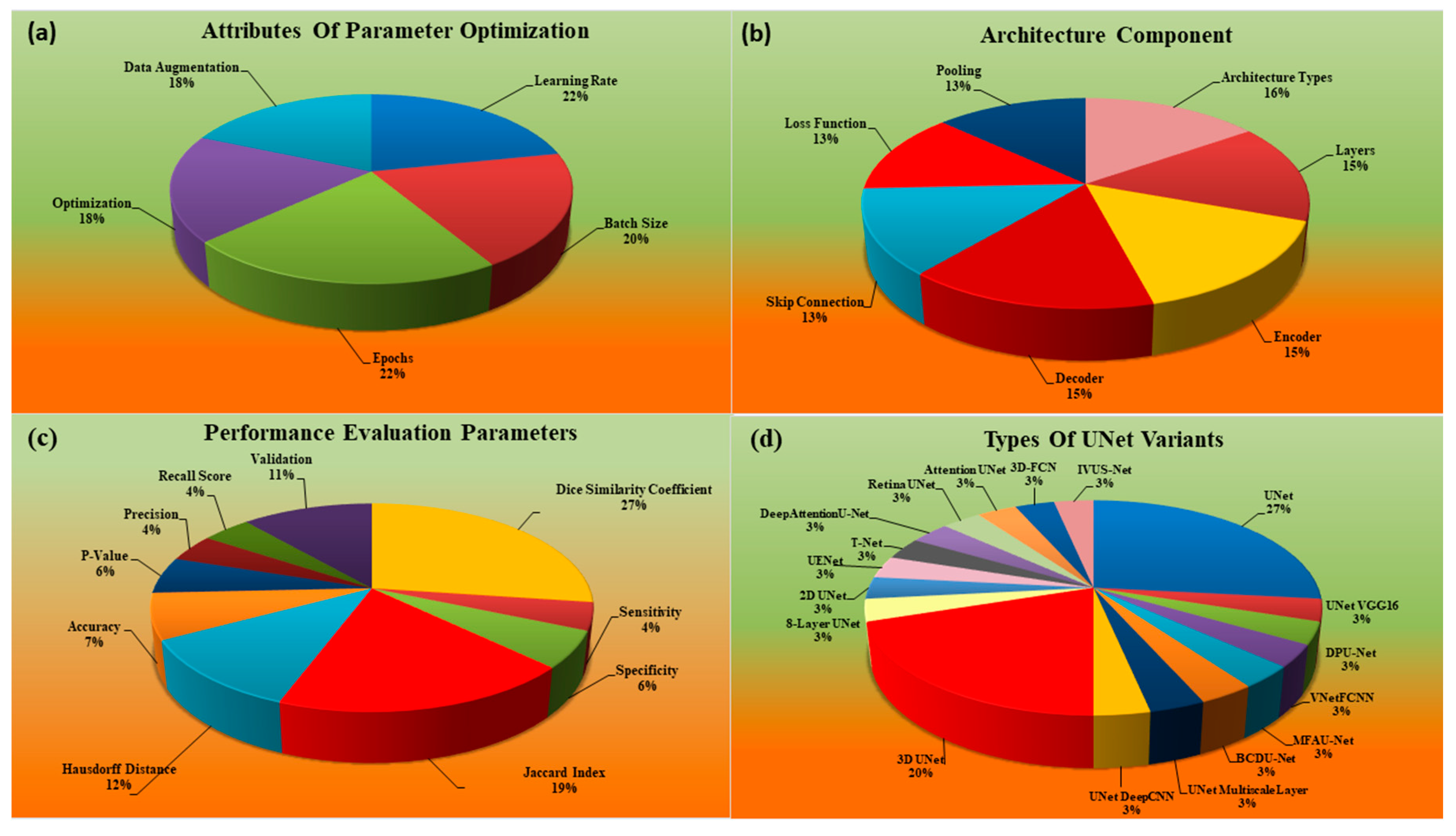
2.2. Statistical Distribution Analysis
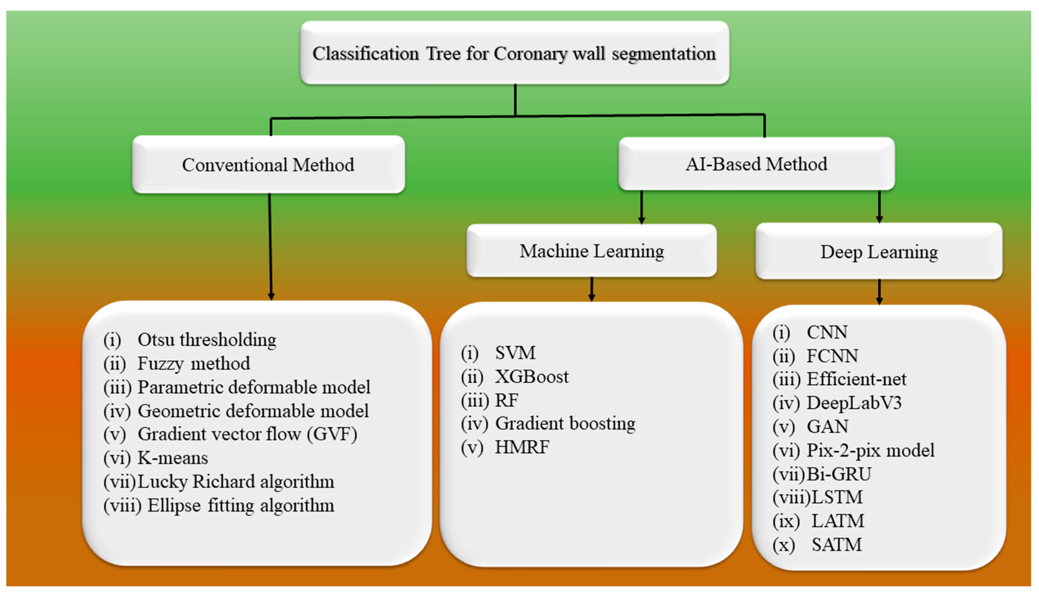
3. Methodology
3.1. Architecture for Wall Segmentation Using Conventional Methods
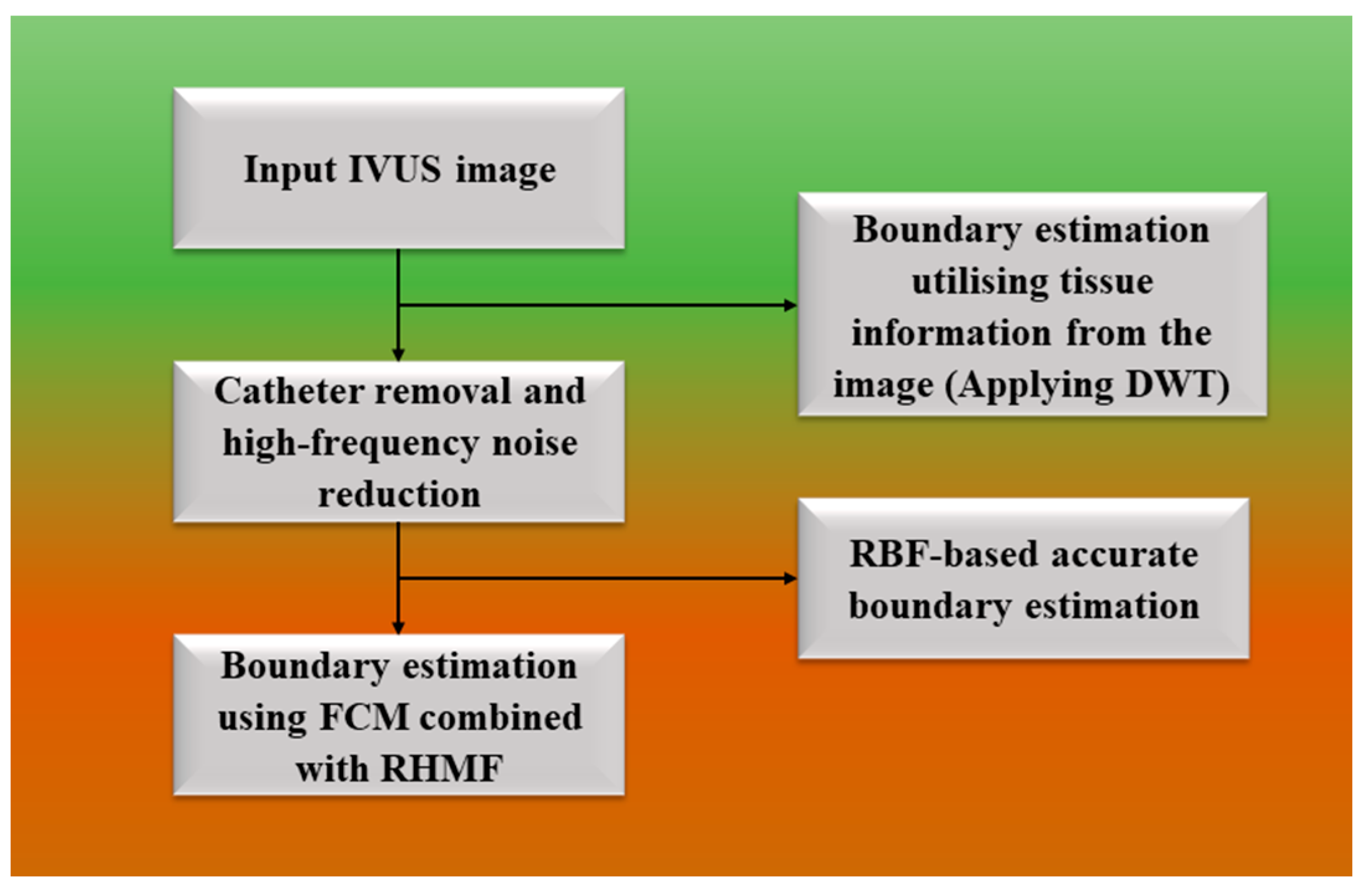
3.1.1. Fuzzy Approach for Wall Segmentation
3.1.2. Parametric Models
3.1.3. Geometric Approach
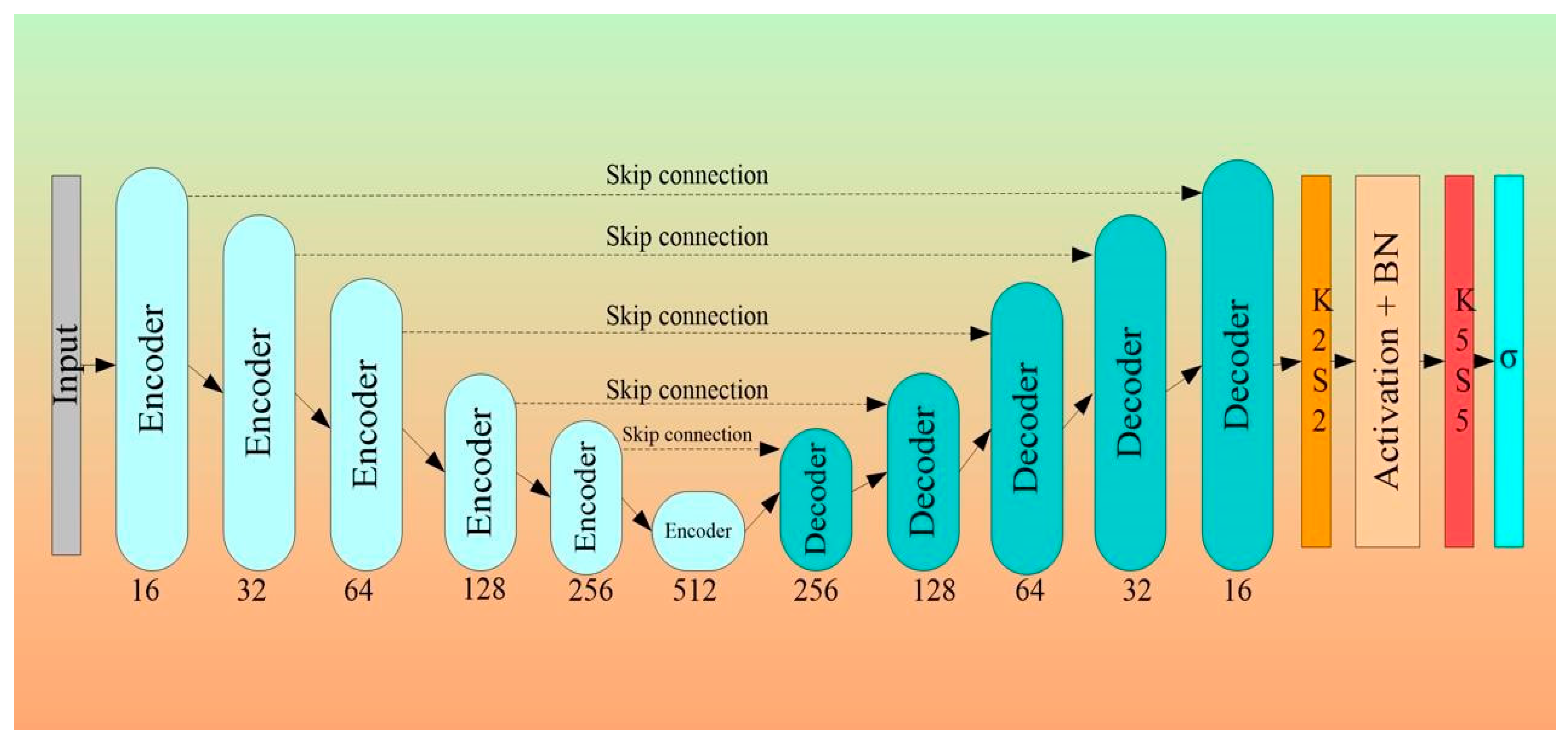
3.2. Architectural Design for 2D Wall Segmentation Using UNet-Based DL System
- The Encoder Block
- The Decoder Block
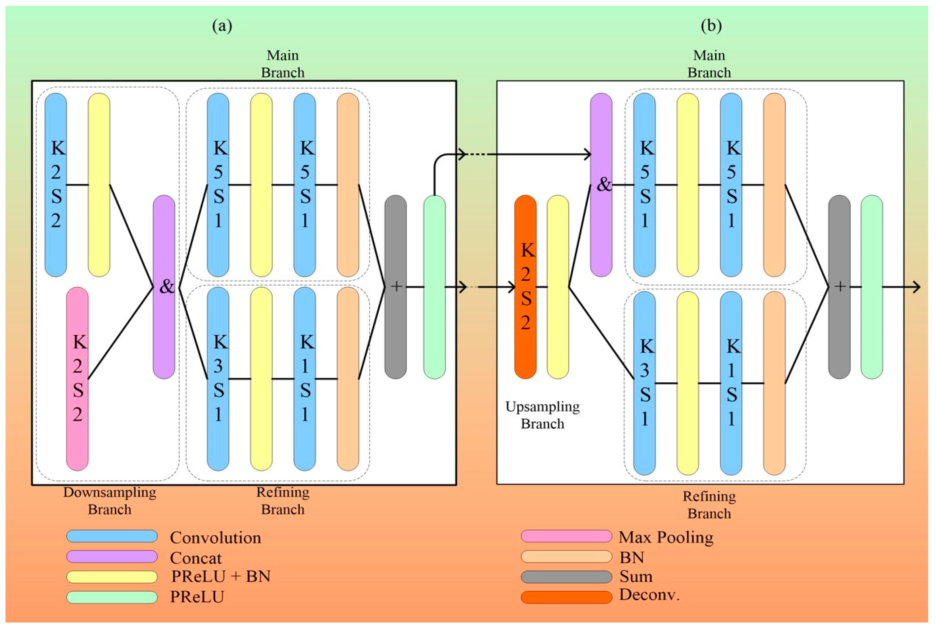
3.2.1. MFAUNet
- Architecture of MFAUNet
- Encoding and Decoding Path
- Feature Aggregation Module.
3.2.2. Dual-Path UNet
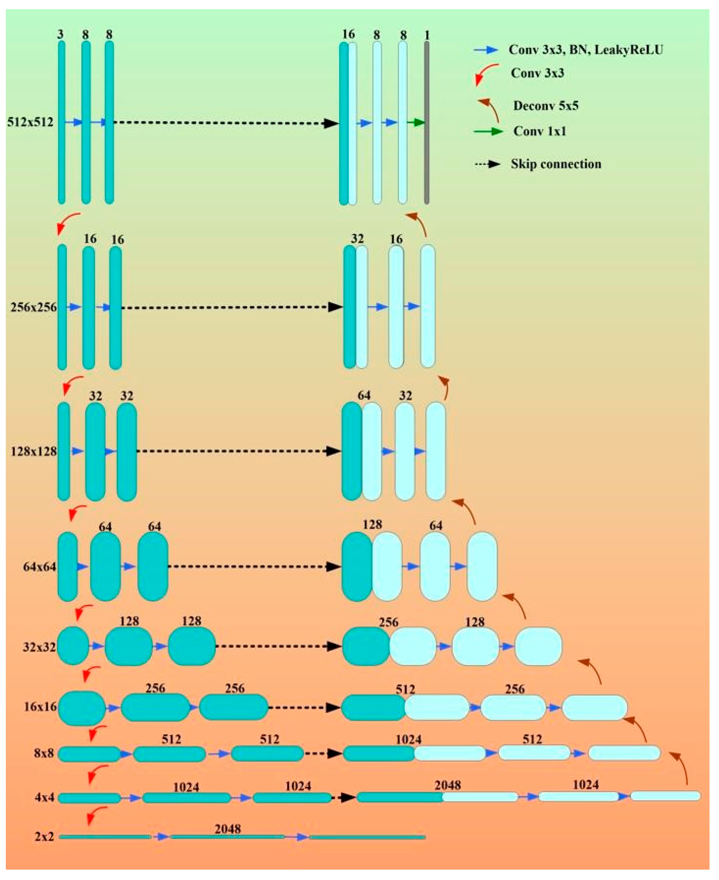
3.2.3. Eight-Layer UNet
- Network architectures of eight-layer UNet
4. Characteristics of UNet and Conventional DL Systems for CAD
4.1. A Special Note on Limitations of Conventional Models and Benefits of AI-Based Solutions
4.2. A Special Note on Quality Control for AI Systems
5. Risk of Bias in Deep-Learning-Based Technologies for Coronary Artery Disease
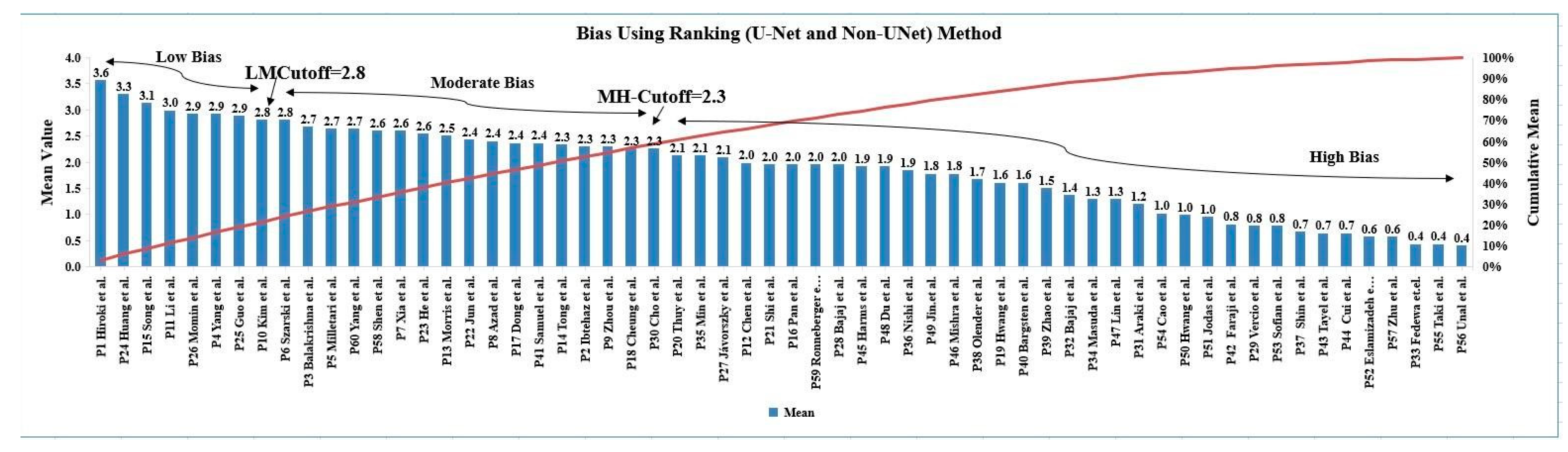
5.1. Risk of Bias via Ranking Method
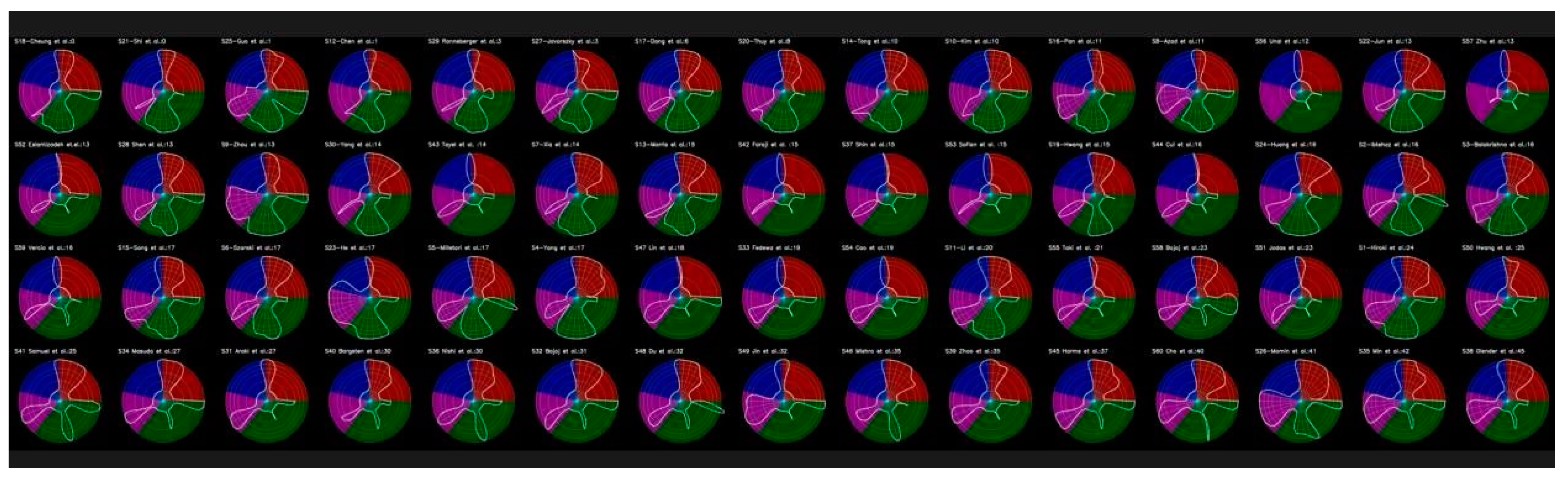
5.2. Radial Bias Map Method
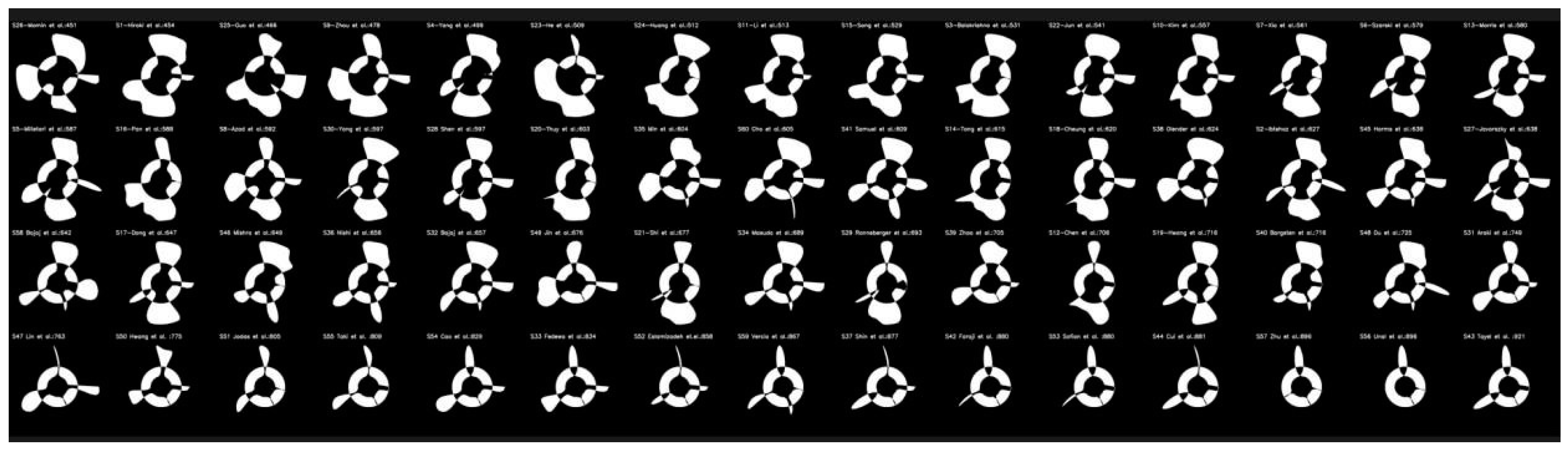
5.3. Radial Bias Area Method
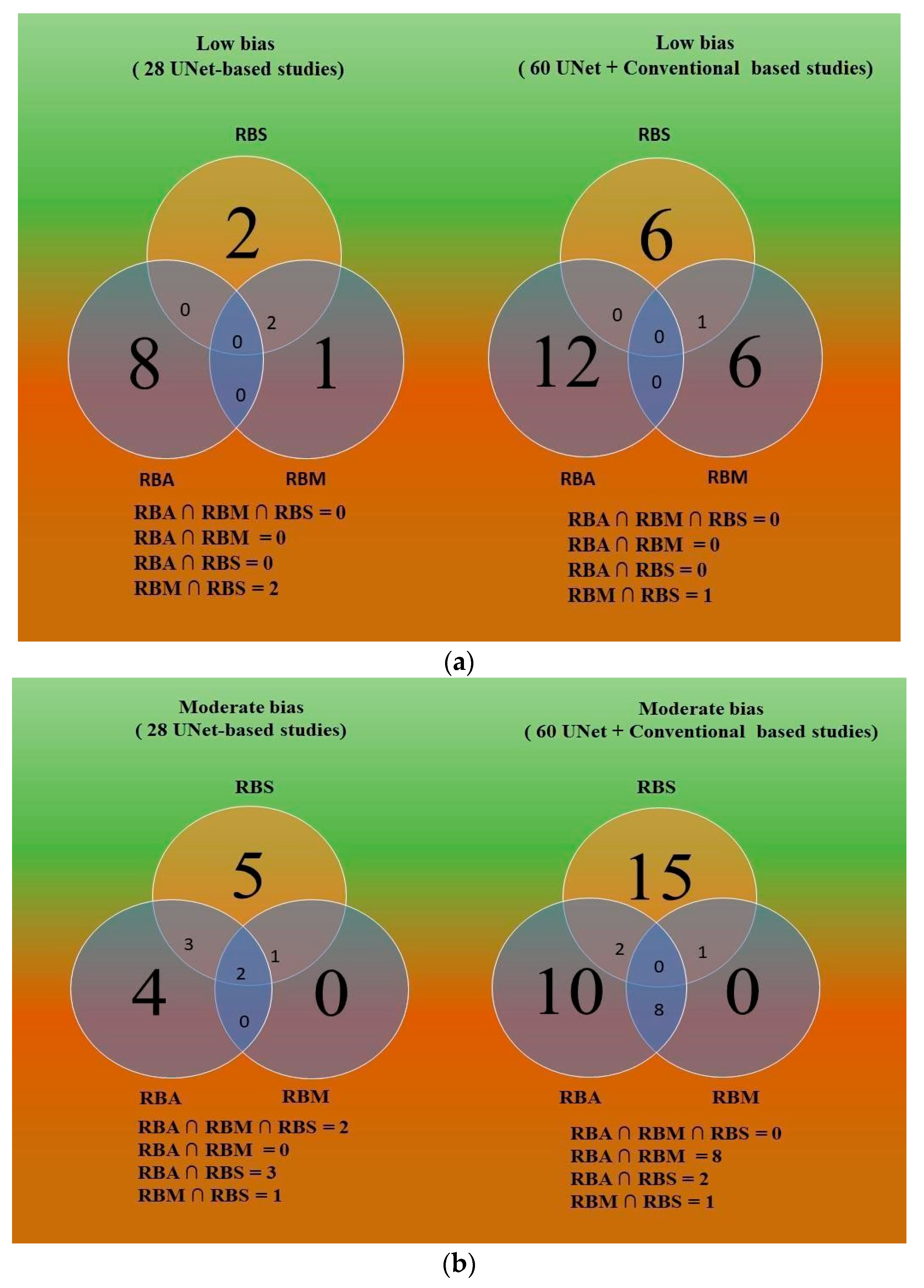
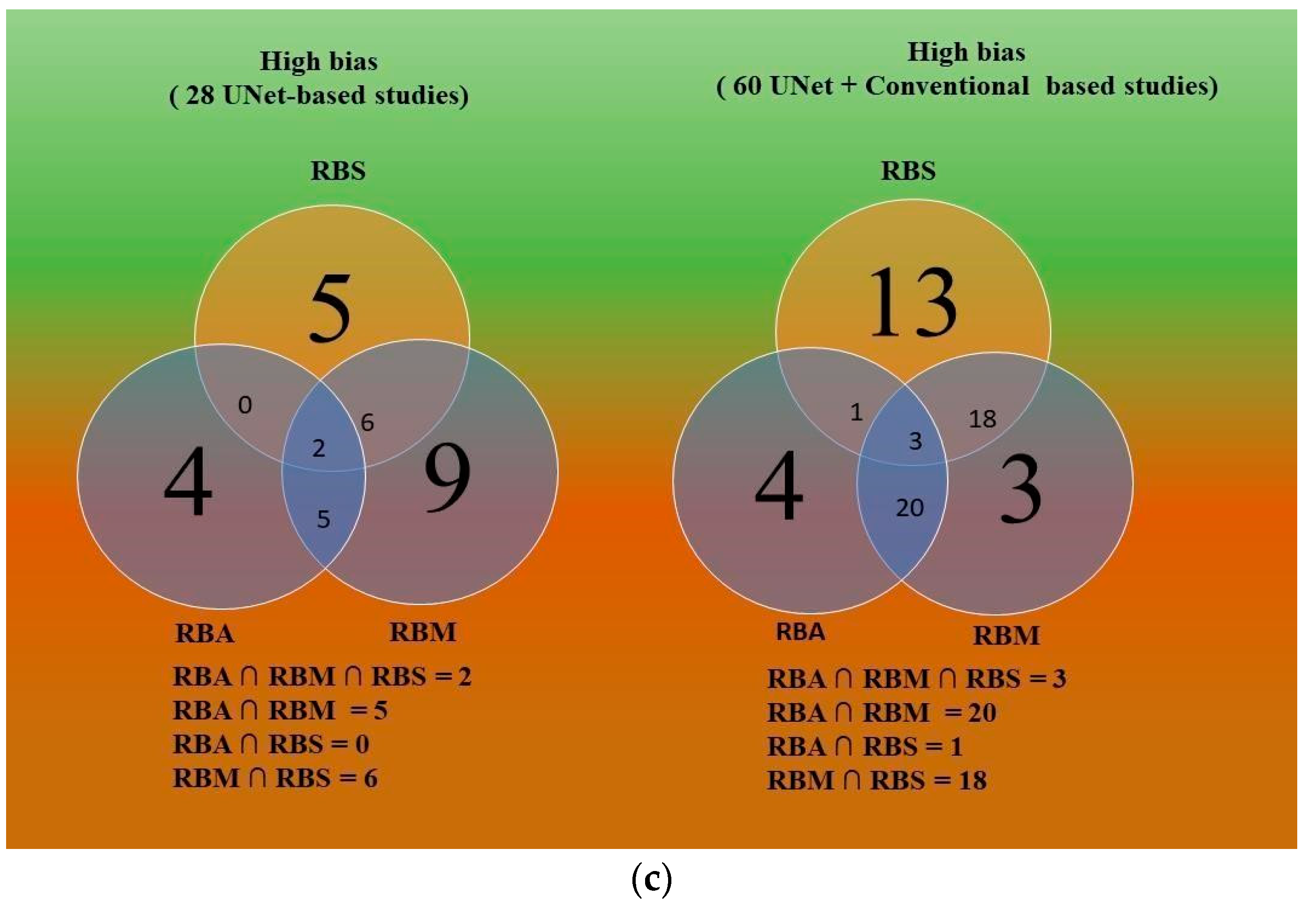
5.4. Comparative study of Three Bias Strategies Based on Venn Diagram
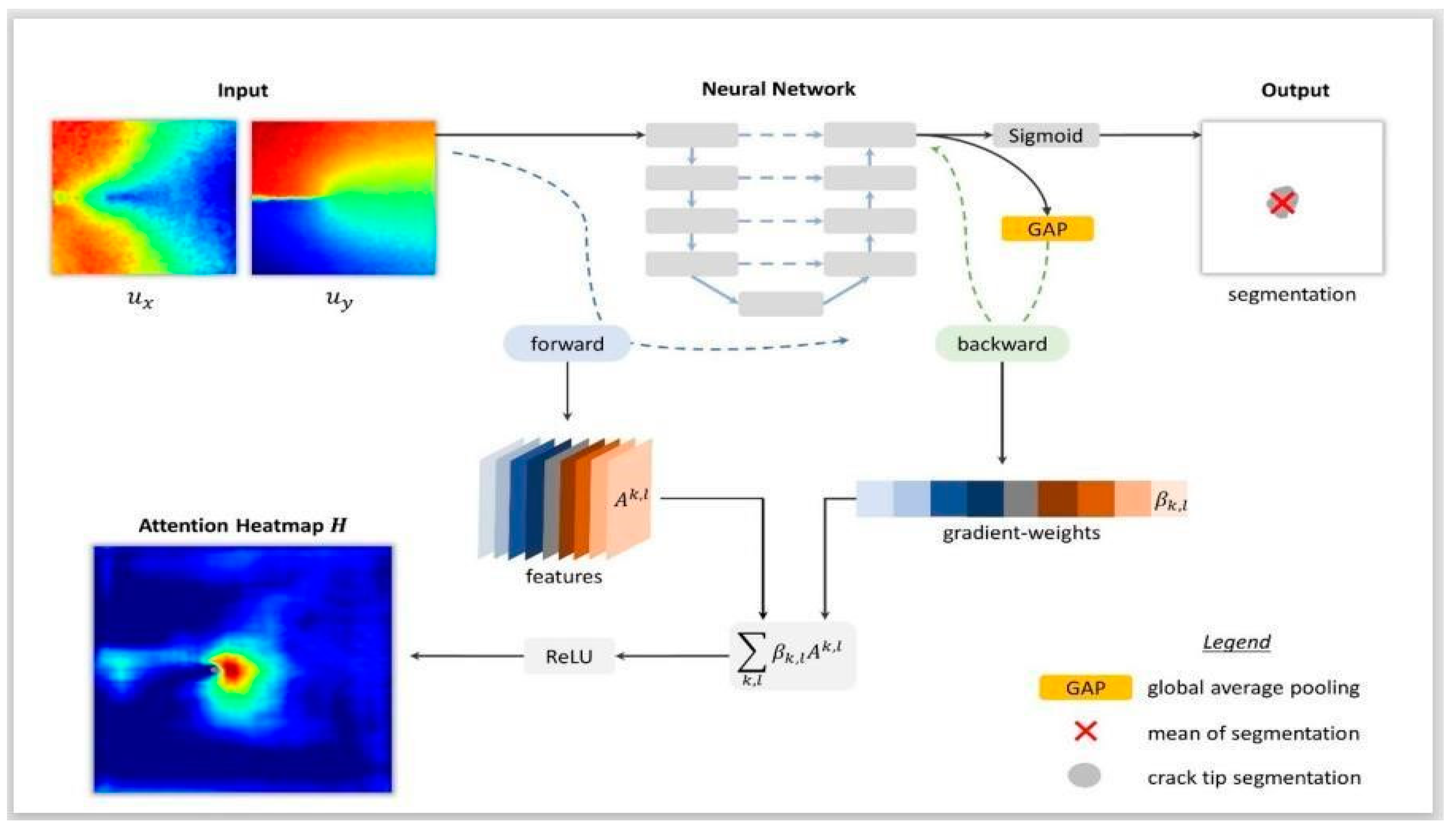
6. Explainability in AI
7. Pruning in Wall Segmentation of IVUS Scan
8. Critical Discussion
8.1. Principal Findings
8.2. Benchmarking
8.3. A Special Note on Comparison of the Latest Deep Learning Solution vs. UNet-Based Models
8.4. A Short Note on UNet and Its Ability
8.5. A Special Note on Machine Learning
8.6. A Special Note on the Differences between Machine Learning (ML) and Deep Learning (DL) Features
8.7. Pros and Cons of Conventional and AI Systems
8.8. Advantage of the UNet Architecture
8.9. A Short Note on Unsupervised Paradigms
8.10. Strengths, Weakness, and Extensions
9. Conclusions
Supplementary Materials
Author Contributions
Funding
Institutional Review Board Statement
Informed Consent Statement
Data Availability Statement
Conflicts of Interest
Appendix A. Ranking Tables

| Studies | Mean | Cumulative Mean | Rank |
|---|---|---|---|
| Shinohara et al. [62] | 3.6 | 3.6 | 1 |
| Huang et al. [67] | 3.3 | 6.9 | 2 |
| Song et al. [24] | 3.1 | 10 | 3 |
| Li et al. [47] | 3.0 | 13 | 4 |
| Momin et al. [58] | 2.9 | 15.9 | 5 |
| Yang et al. [55] | 2.9 | 18.8 | 6 |
| Guo et al. [99] | 2.9 | 21.7 | 7 |
| Kim et al. [48] | 2.8 | 24.5 | 8 |
| Szarski et al. [54] | 2.8 | 27.3 | 9 |
| Balakrishna et al. [46] | 2.7 | 30 | 10 |
| Milletari et al. [53] | 2.7 | 32.7 | 11 |
| Yang et al. [66] | 2.7 | 35.4 | 12 |
| Shen et al. [56] | 2.6 | 38 | 13 |
| Xia et al. [71] | 2.6 | 40.6 | 14 |
| He et al. [44] | 2.6 | 43.2 | 15 |
| Morris et al. [51] | 2.5 | 45.7 | 16 |
| Jun et al. [59] | 2.4 | 48.1 | 17 |
| Dong et al. [61] | 2.4 | 50.5 | 18 |
| Tong et al. [50] | 2.3 | 52.8 | 19 |
| Ibtehaz et al. [45] | 2.3 | 55.1 | 20 |
| Zhou et al. [52] | 2.3 | 57.4 | 21 |
| Cheung et al. [60] | 2.3 | 59.7 | 22 |
| Thuy et al. [68] | 2.1 | 61.8 | 23 |
| Jávorszky et al. [57] | 2.1 | 63.9 | 24 |
| Chen et al. [49] | 2.0 | 65.9 | 25 |
| Shi et al. [64] | 2.0 | 67.9 | 26 |
| Pan et al. [70] | 2.0 | 69.9 | 27 |
| Hwang et al. [69] | 1.6 | 71.5 | 28 |
| Studies | Mean | Cumulative Mean | Rank |
|---|---|---|---|
| Cho et al. [75] | 2.10 | 2.10 | 1 |
| Samuel et al. [96] | 2.10 | 4.20 | 2 |
| Olender et al. [81] | 2.07 | 6.27 | 3 |
| Min et al. [79] | 1.97 | 8.24 | 4 |
| Harms et al. [86] | 1.83 | 10.07 | 5 |
| Bajaj et al. [74] | 1.72 | 11.79 | 6 |
| Bajaj et al. [76] | 1.69 | 13.48 | 7 |
| Jin et al. [95] | 1.69 | 15.17 | 8 |
| Nishi et al. [80] | 1.69 | 16.86 | 9 |
| Mishra et al. [87] | 1.62 | 18.48 | 10 |
| Masuda et al. [78] | 1.59 | 20.07 | 11 |
| Du et al. [98] | 1.52 | 21.59 | 12 |
| Zhao et al. [82] | 1.38 | 22.97 | 13 |
| Bargsten et al. [83] | 1.34 | 24.31 | 14 |
| Lin et al. [97] | 1.24 | 25.55 | 15 |
| Araki et al. [43] | 1.17 | 26.72 | 16 |
| Cao et al. [91] | 0.97 | 27.69 | 17 |
| Fedewa et al. [77] | 0.97 | 28.66 | 18 |
| Hwang et al. [120] | 0.93 | 29.59 | 19 |
| Vercio et al. [65] | 0.79 | 30.38 | 20 |
| Taki et al. [92] | 0.76 | 31.14 | 21 |
| Jodas et al. [88] | 0.72 | 31.86 | 22 |
| Cui et al. [85] | 0.66 | 32.52 | 23 |
| Tayel et al. [84] | 0.66 | 33.18 | 24 |
| Faraji et al. [28] | 0.66 | 33.84 | 25 |
| Shin et al. [111] | 0.66 | 34.50 | 26 |
| Sofian et al. [90] | 0.62 | 35.12 | 27 |
| Eslamizadeh et al. [89] | 0.59 | 35.71 | 28 |
| Zhu et al. [94] | 0.45 | 36.16 | 29 |
| Unal et al. [93] | 0.41 | 36.57 | 30 |
Appendix B
| SN | Acronym | Definition | SN | Acronym | Definition |
|---|---|---|---|---|---|
| 1 | AGs | Attention gates | 33 | LATM | Location-adaptive threshold method |
| 2 | AI | Artificial intelligence | 34 | LI | Lumen-intima |
| 3 | Bi-GRU | Bidirectional gated recurrent unit | 35 | LSTM | Long short-term memory |
| 4 | BN | Batch normalization | 36 | MA | Media-adventitia |
| 5 | CAD | Coronary artery disease | 37 | MFAUNet | Multi-scale feature aggregated UNet |
| 6 | CCTA | Coronary CT angiography | 38 | MI | Myocardial infarction |
| 7 | CKD | Chronic kidney diseases | 39 | ML | Machine learning |
| 8 | CNN | Convolutional neural network | 40 | MRI | Magnetic resonance imaging |
| 9 | CSA | Cross-sectional area | 41 | NB | Naïve Bayes |
| 10 | CT | Computed tomography | 42 | NIRS | Near-infrared spectroscopy |
| 11 | CVD | Cardiovascular disease | 43 | PCA | Principle component analysis |
| 12 | DCNN | Deep convolutional neural network | 44 | PCI | Percutaneous coronary intervention |
| 13 | DL | Deep learning | 45 | PReLU | Parametric rectified linear unit |
| 14 | DPUNet | Dual-path UNet | 46 | PSO | Particle swarm optimization |
| 15 | EAT | Epicardial adipose tissue | 47 | RA | Rheumatoid arthritis |
| 16 | EEM | External elastic membrane | 48 | RF | Random forest |
| 17 | EREL | Extremal area of extremum level | 49 | RNN | Recurrent neural network |
| 18 | FAM | Feature aggregated module | 50 | RoB | Risk of bias |
| 19 | FCM | Fuzzy c-means | 51 | RPN | Regional proposal network |
| 20 | FCNN | Fully convolutional neural network | 52 | RRS | Random radius symmetry |
| 21 | FNs | False negatives | 53 | RUS | Random undersampling |
| 22 | FPs | False positives | 54 | SATM | Scan-adaptive threshold method |
| 23 | GA | Genetic algorithm | 55 | SDL | Solo deep learning |
| 24 | GAN | Generative adversarial network | 56 | SVM | Support vector machine |
| 25 | GT | Ground truth | 57 | TL | Transfer learning |
| 26 | GVF | Gradient vector flow | 58 | US | Ultrasound |
| 27 | HDL | Hybrid deep learning | 59 | VGG | Visual geometric group |
| 28 | HMRF | Hidden Markov random field | 60 | VH | Virtual histology |
| 29 | IMTV | Intima-media thickness variability | 61 | VSSC-Net | Vessel-specific skip chain network |
| 30 | IVOCT | Intravascular optical CT | 62 | WO | Whale optimization |
| 31 | IVUS | Intravascular ultrasound | 63 | XAI | Explainable AI |
| 32 | KNN | K-nearest neighbors | 64 | XCA | X-ray coronary angiography |
- Fuzzy approach
- Parametric approach
- Geometric approach
Appendix C
Appendix D
- Pruning Training Models
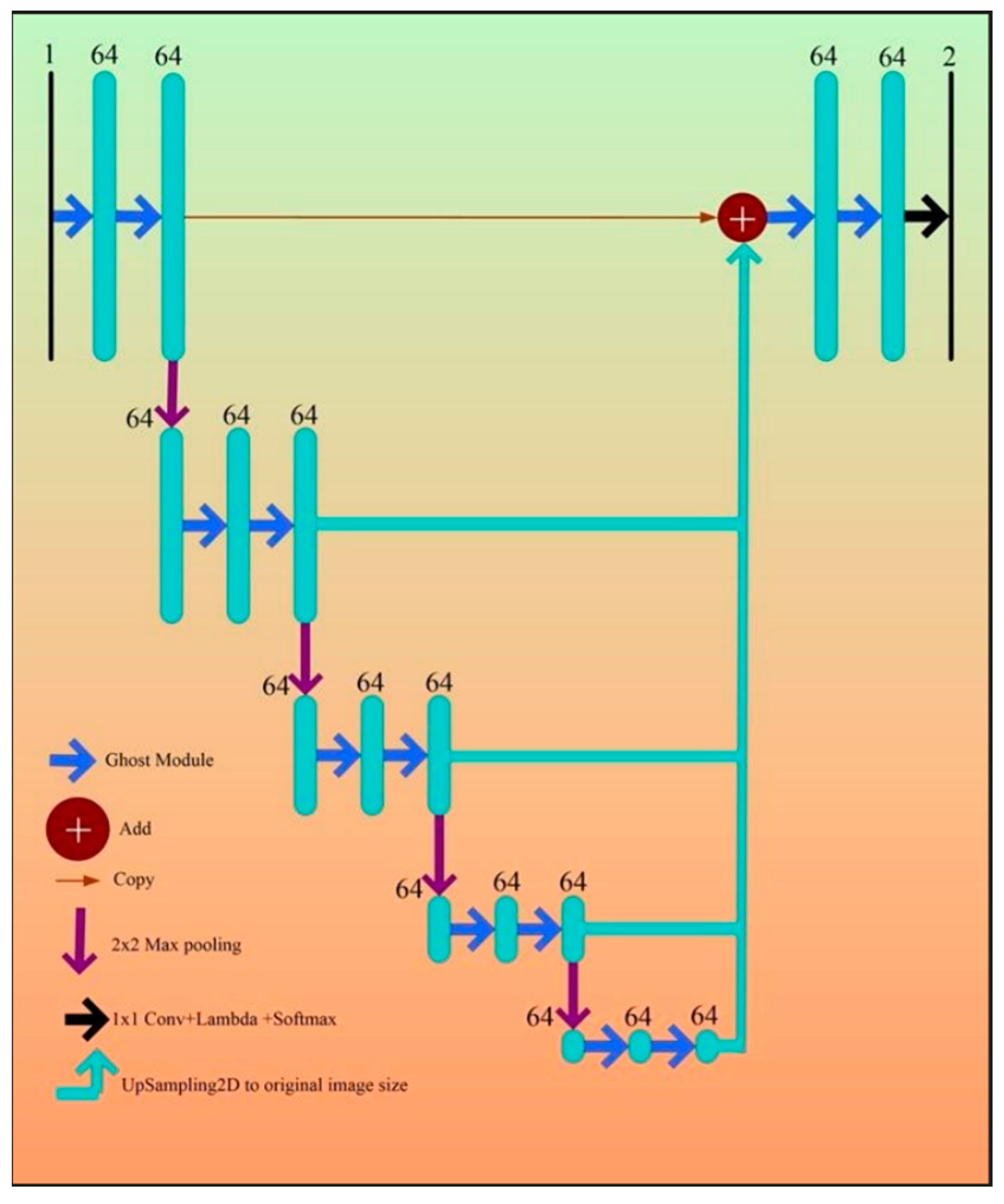
Appendix E. Half-UNet Concepts
Appendix F. Bias Assessment
References
- Smith, S.C., Jr.; Collins, A.; Ferrari, R.; Holmes, D.R., Jr.; Logstrup, S.; McGhie, D.V.; Ralston, J.; Sacco, R.L.; Stam, H.; Taubert, K. Our time: A call to save preventable death from cardiovascular disease (heart disease and stroke). Circulation 2012, 126, 2769–2775. [Google Scholar] [CrossRef] [PubMed]
- Chan, M.Y.; Du, X.; Eccleston, D.; Ma, C.; Mohanan, P.P.; Ogita, M.; Shyu, K.-G.; Yan, B.P.; Jeong, Y.-H. Acute coronary syndrome in the Asia-Pacific region. Int. J. Cardiol. 2016, 202, 861–869. [Google Scholar] [CrossRef] [PubMed]
- Suri, J.S.; Kathuria, C.; Molinari, F. (Eds.) Atherosclerosis Disease Management; Springer Science & Business Media: Berlin, Germany, 2010. [Google Scholar]
- Kandaswamy, E.; Zuo, L. Recent advances in treatment of coronary artery disease: Role of science and technology. Int. J. Mol. Sci. 2018, 19, 424. [Google Scholar] [CrossRef] [PubMed]
- Katouzian, A.; Angelini, E.D.; Carlier, S.G.; Suri, J.S.; Navab, N.; Laine, A.F. A state-of-the-art review on segmentation algorithms in intravascular ultrasound (IVUS) images. IEEE Trans. Inf. Technol. Biomed. 2012, 16, 823–834. [Google Scholar] [CrossRef] [PubMed]
- Darmoch, F.; Alraies, M.C.; Al-Khadra, Y.; Moussa Pacha, H.; Pinto, D.S.; Osborn, E.A. Intravascular ultrasound imaging–guided versus coronary angiography–guided percutaneous coronary intervention: A systematic review and meta-analysis. J. Am. Heart Assoc. 2020, 9, e013678. [Google Scholar] [CrossRef]
- Escolar, E.; Weigold, G.; Fuisz, A.; Weissman, N.J. New imaging techniques for diagnosing coronary artery disease. CMAJ 2006, 174, 487–495. [Google Scholar] [CrossRef]
- Banchhor, S.K.; Londhe, N.D.; Araki, T.; Saba, L.; Radeva, P.; Laird, J.R.; Suri, J.S. Well-balanced system for coronary calcium detection and volume measurement in a low resolution intravascular ultrasound videos. Comput. Biol. Med. 2017, 84, 168–181. [Google Scholar] [CrossRef]
- Boi, A.; Jamthikar, A.D.; Saba, L.; Gupta, D.; Sharma, A.; Loi, B.; Laird, J.R.; Khanna, N.N.; Suri, J.S. A survey on coronary atherosclerotic plaque tissue characterization in intravascular optical coherence tomography. Curr. Atheroscler. Rep. 2018, 20, 1–17. [Google Scholar] [CrossRef]
- Saba, L.; Suri, J.S. Multi-Detector CT Imaging: Principles, Head, Neck, and Vascular Systems; CRC Press: Boca Raton, FL, USA, 2013; Volume 1. [Google Scholar]
- Saba, L.; Agarwal, N.; Cau, R.; Gerosa, C.; Sanfilippo, R.; Porcu, M.; Montisci, R.; Cerrone, G.; Qi, Y.; Balestrieri, A. Review of imaging biomarkers for the vulnerable carotid plaque. JVS Vasc. Sci. 2021, 2, 149–158. [Google Scholar] [CrossRef]
- Caredda, G.; Bassareo, P.P.; Cherchi, M.V.; Pontone, G.; Suri, J.S.; Saba, L. Anderson-fabry disease: Role of traditional and new cardiac MRI techniques. Br. J. Radiol. 2021, 94, 20210020. [Google Scholar] [CrossRef]
- Cau, R.; Cherchi, V.; Micheletti, G.; Porcu, M.; Mannelli, L.; Bassareo, P.; Suri, J.S.; Saba, L. Potential role of artificial intelligence in cardiac magnetic resonance imaging: Can it help clinicians in making a diagnosis? J. Thorac. Imaging 2021, 36, 142–148. [Google Scholar] [CrossRef] [PubMed]
- Laine, A.; Sanches, J.M.; Suri, J.S. Ultrasound Imaging: Advances and Applications; Springer: Cham, Seitzerland, 2012. [Google Scholar]
- Radeva, P.; Suri, J.S. Vascular and Intravascular Imaging Trends, Analysis, and Challenges: Plaque Characterization; IOP Publishing: Bristol, UK, 2019; Volume 2. [Google Scholar]
- Sun, Z.; Xu, L. Coronary CT angiography in the quantitative assessment of coronary plaques. BioMed Res. Int. 2014, 2014, 346380. [Google Scholar] [CrossRef] [PubMed]
- Cau, R.; Flanders, A.; Mannelli, L.; Politi, C.; Faa, G.; Suri, J.S.; Saba, L. Artificial intelligence in computed tomography plaque characterization: A review. Eur. J. Radiol. 2021, 140, 109767. [Google Scholar] [CrossRef] [PubMed]
- Murgia, A.; Balestrieri, A.; Crivelli, P.; Suri, J.S.; Conti, M.; Cademartiri, F.; Saba, L. Cardiac computed tomography radiomics: An emerging tool for the non-invasive assessment of coronary atherosclerosis. Cardiovasc. Diagn. Ther. 2020, 10, 2005. [Google Scholar] [CrossRef] [PubMed]
- Onnis, C.; Cadeddu Dessalvi, C.; Cademartiri, F.; Muscogiuri, G.; Angius, S.; Contini, F.; Suri, J.S.; Sironi, S.; Salgado, R.; Esposito, A. Quantitative and qualitative features of carotid and coronary atherosclerotic plaque among men and women. Front. Cardiovasc. Med. 2022, 9, 970438. [Google Scholar] [CrossRef]
- Onnis, C.; Muscogiuri, G.; Bassareo, P.P.; Cau, R.; Mannelli, L.; Cadeddu, C.; Suri, J.S.; Cerrone, G.; Gerosa, C.; Sironi, S. Non-invasive coronary imaging in patients with COVID-19: A narrative review. Eur. J. Radiol. 2022, 149, 110188. [Google Scholar] [CrossRef]
- Ghekiere, O.; Salgado, R.; Buls, N.; Leiner, T.; Mancini, I.; Vanhoenacker, P.; Dendale, P.; Nchimi, A. Image quality in coronary CT angiography: Challenges and technical solutions. Br. J. Radiol. 2017, 90, 20160567. [Google Scholar] [CrossRef]
- Ozolanta, I.; Tetere, G.; Purinya, B.; Kasyanov, V. Changes in the mechanical properties, biochemical contents and wall structure of the human coronary arteries with age and sex. Med. Eng. Phys. 1998, 20, 523–533. [Google Scholar] [CrossRef]
- Hayes, S.N.; Kim, E.S.; Saw, J.; Adlam, D.; Arslanian-Engoren, C.; Economy, K.E.; Ganesh, S.K.; Gulati, R.; Lindsay, M.E.; Mieres, J.H. Spontaneous coronary artery dissection: Current state of the science: A scientific statement from the American Heart Association. Circulation 2018, 137, e523–e557. [Google Scholar] [CrossRef]
- Song, A.; Xu, L.; Wang, L.; Wang, B.; Yang, X.; Xu, B.; Yang, B.; Greenwald, S.E. Automatic Coronary Artery Segmentation of CCTA Images with an Efficient Feature-Fusion-and-Rectification 3D-UNet. IEEE J. Biomed. Health Inform. 2022, 26, 4044–4055. [Google Scholar] [CrossRef]
- Schroeder, S.; Kopp, A.F.; Kuettner, A.; Burgstahler, C.; Herdeg, C.; Heuschmid, M.; Baumbach, A.; Claussen, C.D.; Karsch, K.R.; Seipel, L. Influence of heart rate on vessel visibility in noninvasive coronary angiography using new multislice computed tomography: Experience in 94 patients. Clin. Imaging 2002, 26, 106–111. [Google Scholar] [CrossRef] [PubMed]
- Araki, T.; Ikeda, N.; Shukla, D.; Londhe, N.D.; Shrivastava, V.K.; Banchhor, S.K.; Saba, L.; Nicolaides, A.; Shafique, S.; Laird, J.R. A new method for IVUS-based coronary artery disease risk stratification: A link between coronary & carotid ultrasound plaque burdens. Comput. Methods Programs Biomed. 2016, 124, 161–179. [Google Scholar] [PubMed]
- Ono, M.; Kawashima, H.; Hara, H.; Gao, C.; Wang, R.; Kogame, N.; Takahashi, K.; Chichareon, P.; Modolo, R.; Tomaniak, M. Advances in IVUS/OCT and future clinical perspective of novel hybrid catheter system in coronary imaging. Front. Cardiovasc. Med. 2020, 7, 119. [Google Scholar] [CrossRef] [PubMed]
- Faraji, M.; Cheng, I.; Naudin, I.; Basu, A. Segmentation of arterial walls in intravascular ultrasound cross-sectional images using extremal region selection. Ultrasonics 2018, 84, 356–365. [Google Scholar] [CrossRef] [PubMed]
- Suri, J.S.; Paul, S.; Maindarkar, M.A.; Puvvula, A.; Saxena, S.; Saba, L.; Turk, M.; Laird, J.R.; Khanna, N.N.; Viskovic, K. Cardiovascular/stroke risk stratification in Parkinson’s disease patients using atherosclerosis pathway and artificial intelligence paradigm: A systematic review. Metabolites 2022, 12, 312. [Google Scholar] [CrossRef] [PubMed]
- Jena, B.; Saxena, S.; Nayak, G.K.; Balestrieri, A.; Gupta, N.; Khanna, N.N.; Laird, J.R.; Kalra, M.K.; Fouda, M.M.; Saba, L.; et al. Brain Tumor Characterization Using Radiogenomics in Artificial Intelligence Framework. Cancers 2022, 14, 4052. [Google Scholar] [CrossRef] [PubMed]
- Suri, J.S.; Maindarkar, M.A.; Paul, S.; Ahluwalia, P.; Bhagawati, M.; Saba, L.; Faa, G.; Saxena, S.; Singh, I.M.; Chadha, P.S. Deep Learning Paradigm for Cardiovascular Disease/Stroke Risk Stratification in Parkinson’s Disease Affected by COVID-19: A Narrative Review. Diagnostics 2022, 12, 1543. [Google Scholar] [CrossRef] [PubMed]
- Suri, J.S.; Bhagawati, M.; Paul, S.; Protogerou, A.D.; Sfikakis, P.P.; Kitas, G.D.; Khanna, N.N.; Ruzsa, Z.; Sharma, A.M.; Saxena, S. A powerful paradigm for cardiovascular risk stratification using multiclass, multi-label, and ensemble-based machine learning paradigms: A narrative review. Diagnostics 2022, 12, 722. [Google Scholar] [CrossRef]
- Das, S.; Nayak, G.K.; Saba, L.; Kalra, M.; Suri, J.S.; Saxena, S. An artificial intelligence framework and its bias for brain tumor segmentation: A narrative review. Comput. Biol. Med. 2022, 143, 105273. [Google Scholar] [CrossRef]
- Suri, J.S.; Agarwal, S.; Jena, B.; Saxena, S.; El-Baz, A.; Agarwal, V.; Kalra, M.K.; Saba, L.; Viskovic, K.; Fatemi, M. Five strategies for bias estimation in artificial intelligence-based hybrid deep learning for acute respiratory distress syndrome COVID-19 lung infected patients using AP (AI) Bias 2.0: A systematic review. In IEEE Transactions on Instrumentation and Measurement; IEEE: Piscataway, NJ, USA, 2022. [Google Scholar] [CrossRef]
- Suri, J.S.; Agarwal, S.; Gupta, S.K.; Puvvula, A.; Viskovic, K.; Suri, N.; Alizad, A.; El-Baz, A.; Saba, L.; Fatemi, M. Systematic review of artificial intelligence in acute respiratory distress syndrome for COVID-19 lung patients: A biomedical imaging perspective. IEEE J. Biomed. Health Inform. 2021, 25, 4128–4139. [Google Scholar] [CrossRef]
- Ikeda, N.; Gupta, A.; Dey, N.; Bose, S.; Shafique, S.; Arak, T.; Godia, E.C.; Saba, L.; Laird, J.R.; Nicolaides, A. Improved correlation between carotid and coronary atherosclerosis SYNTAX score using automated ultrasound carotid bulb plaque IMT measurement. Ultrasound Med. Biol. 2015, 41, 1247–1262. [Google Scholar] [CrossRef] [PubMed]
- Ikeda, N.; Araki, T.; Sugi, K.; Nakamura, M.; Deidda, M.; Molinari, F.; Meiburger, K.M.; Acharya, U.R.; Saba, L.; Bassareo, P.P. Ankle–brachial index and its link to automated carotid ultrasound measurement of intima–media thickness variability in 500 Japanese coronary artery disease patients. Curr. Atheroscler. Rep. 2014, 16, 1–8. [Google Scholar] [CrossRef] [PubMed]
- Kumar, A.; Aelgani, V.; Vohra, R.; Gupta, S.K.; Bhagawati, M.; Paul, S.; Saba, L.; Suri, N.; Khanna, N.N.; Laird, J.R. Artificial intelligence bias in medical system designs: A systematic review. Multimedia Tools and Applications. 2023, 347, 1–53. [Google Scholar] [CrossRef]
- Suri, J.S.; Bhagawati, M.; Agarwal, S.; Paul, S.; Pandey, A.; Gupta, S.K.; Saba, L.; Paraskevas, K.I.; Khanna, N.N.; Laird, J.R. UNet Deep Learning Architecture for Segmentation of Vascular and Non-Vascular Images: A Microscopic Look at UNet Components Buffered With Pruning, Explainable Artificial Intelligence, and Bias. IEEE Access 2022, 11, 595–645. [Google Scholar] [CrossRef]
- Sanagala, S.S.; Nicolaides, A.; Gupta, S.K.; Koppula, V.K.; Saba, L.; Agarwal, S.; Johri, A.M.; Kalra, M.S.; Suri, J.S. Ten fast transfer learning models for carotid ultrasound plaque tissue characterization in augmentation framework embedded with heatmaps for stroke risk stratification. Diagnostics 2021, 11, 2109. [Google Scholar] [CrossRef]
- Suri, J.S.; Agarwal, S.; Chabert, G.L.; Carriero, A.; Paschè, A.; Danna, P.S.; Saba, L.; Mehmedović, A.; Faa, G.; Singh, I.M. COVLIAS 2.0-cXAI: Cloud-based explainable deep learning system for COVID-19 lesion localization in computed tomography scans. Diagnostics 2022, 12, 1482. [Google Scholar] [CrossRef]
- Agarwal, M.; Agarwal, S.; Saba, L.; Chabert, G.L.; Gupta, S.; Carriero, A.; Pasche, A.; Danna, P.; Mehmedovic, A.; Faa, G. Eight pruning deep learning models for low storage and high-speed COVID-19 computed tomography lung segmentation and heatmap-based lesion localization: A multicenter study using COVLIAS 2.0. Comput. Biol. Med. 2022, 146, 105571. [Google Scholar] [CrossRef]
- Araki, T.; Banchhor, S.K.; Londhe, N.D.; Ikeda, N.; Radeva, P.; Shukla, D.; Saba, L.; Balestrieri, A.; Nicolaides, A.; Shafique, S. Reliable and accurate calcium volume measurement in coronary artery using intravascular ultrasound videos. J. Med. Syst. 2016, 40, 1–20. [Google Scholar] [CrossRef]
- He, X.; Guo, B.J.; Lei, Y.; Wang, T.; Fu, Y.; Curran, W.J.; Zhang, L.J.; Liu, T.; Yang, X. Automatic segmentation and quantification of epicardial adipose tissue from coronary computed tomography angiography. Phys. Med. Biol. 2020, 65, 095012. [Google Scholar] [CrossRef]
- Ibtehaz, N.; Rahman, M.S. MultiResUNet: Rethinking the U-Net architecture for multimodal biomedical image segmentation. Neural Netw. 2020, 121, 74–87. [Google Scholar] [CrossRef]
- Balakrishna, C.; Dadashzadeh, S.; Soltaninejad, S. Automatic detection of lumen and media in the IVUS images using U-Net with VGG16 Encoder. arXiv 2018, arXiv:1806.07554. [Google Scholar]
- Li, Y.-C.; Shen, T.-Y.; Chen, C.-C.; Chang, W.-T.; Lee, P.-Y.; Huang, C.-C.J. Automatic detection of atherosclerotic plaque and calcification from intravascular ultrasound images by using deep convolutional neural networks. IEEE Trans. Ultrason. Ferroelectr. Freq. Control. 2021, 68, 1762–1772. [Google Scholar] [CrossRef]
- Kim, S.; Jang, Y.; Jeon, B.; Hong, Y.; Shim, H.; Chang, H. Fully automatic segmentation of coronary arteries based on deep neural network in intravascular ultrasound images. In Intravascular Imaging and Computer Assisted Stenting and Large-Scale Annotation of Biomedical Data and Expert Label Synthesis; 7th Joint International Workshop, CVII-STENT 2018 and Third International Workshop, LABELS 2018, Held in Conjunction with MICCAI 2018, Granada, Spain, September 16, 2018, Proceedings 3; Springer International Publishing: Cham, Switzerland, 2018; pp. 161–168. [Google Scholar]
- Chen, Y.-C.; Lin, Y.-C.; Wang, C.-P.; Lee, C.-Y.; Lee, W.-J.; Wang, T.-D.; Chen, C.-M. Coronary artery segmentation in cardiac CT angiography using 3D multi-channel U-net. arXiv 2019, arXiv:1907.12246. [Google Scholar]
- Tong, Q.; Ning, M.; Si, W.; Liao, X.; Qin, J. 3D deeply-supervised U-net based whole heart segmentation. In Statistical Atlases and Computational Models of the Heart. ACDC and MMWHS Challenges: 8th International Workshop, STACOM 2017, Held in Conjunction with MICCAI 2017, Quebec City, Canada, September 10–14, 2017, Revised Selected Papers 8; Springer International Publishing: Cham, Switzerland, 2018; pp. 224–232. [Google Scholar]
- Morris, E.D.; Ghanem, A.I.; Dong, M.; Pantelic, M.V.; Walker, E.M.; Glide-Hurst, C.K. Cardiac substructure segmentation with deep learning for improved cardiac sparing. Med. Phys. 2020, 47, 576–586. [Google Scholar] [CrossRef]
- Zhou, Z.; Siddiquee, M.M.R.; Tajbakhsh, N.; Liang, J. Unet++: Redesigning skip connections to exploit multiscale features in image segmentation. IEEE Trans. Med. Imaging 2019, 39, 1856–1867. [Google Scholar] [CrossRef]
- Milletari, F.; Navab, N.; Ahmadi, S.-A. V-net: Fully convolutional neural networks for volumetric medical image segmentation. In Proceedings of the 2016 Fourth International Conference on 3D Vision (3DV), Stanford, CA, USA, 25–28 October 2016; pp. 565–571. [Google Scholar]
- Szarski, M.; Chauhan, S. Improved real-time segmentation of Intravascular Ultrasound images using coordinate-aware fully convolutional networks. Comput. Med. Imaging Graph. 2021, 91, 101955. [Google Scholar] [CrossRef]
- Yang, J.; Faraji, M.; Basu, A. Robust segmentation of arterial walls in intravascular ultrasound images using Dual Path U-Net. Ultrasonics 2019, 96, 24–33. [Google Scholar] [CrossRef]
- Shen, Y.; Fang, Z.; Gao, Y.; Xiong, N.; Zhong, C.; Tang, X. Coronary arteries segmentation based on 3D FCN with attention gate and level set function. IEEE Access 2019, 7, 42826–42835. [Google Scholar] [CrossRef]
- Jávorszky, N.; Homonnay, B.; Gerstenblith, G.; Bluemke, D.; Kiss, P.; Török, M.; Celentano, D.; Lai, H.; Lai, S.; Kolossváry, M. Deep learning–based atherosclerotic coronary plaque segmentation on coronary CT angiography. Eur. Radiol. 2022, 32, 7217–7226. [Google Scholar] [CrossRef]
- Momin, S.; Lei, Y.; McCall, N.S.; Zhang, J.; Roper, J.; Harms, J.; Tian, S.; Lloyd, M.S.; Liu, T.; Bradley, J.D. Mutual enhancing learning-based automatic segmentation of CT cardiac substructure. Phys. Med. Biol. 2022, 67, 105008. [Google Scholar] [CrossRef]
- Jun Guo, B.; He, X.; Lei, Y.; Harms, J.; Wang, T.; Curran, W.J.; Liu, T.; Jiang Zhang, L.; Yang, X. Automated left ventricular myocardium segmentation using 3D deeply supervised attention U-net for coronary computed tomography angiography; CT myocardium segmentation. Med. Phys. 2020, 47, 1775–1785. [Google Scholar] [CrossRef]
- Cheung, W.K.; Bell, R.; Nair, A.; Menezes, L.J.; Patel, R.; Wan, S.; Chou, K.; Chen, J.; Torii, R.; Davies, R.H. A computationally efficient approach to segmentation of the aorta and coronary arteries using deep learning. IEEE Access 2021, 9, 108873–108888. [Google Scholar] [CrossRef]
- Dong, L.; Jiang, W.; Lu, W.; Jiang, J.; Zhao, Y.; Song, X.; Leng, X.; Zhao, H.; Wang, J.A.; Li, C. Automatic segmentation of coronary lumen and external elastic membrane in intravascular ultrasound images using 8-layer U-Net. BioMedical Eng. OnLine 2021, 20, 1–9. [Google Scholar] [CrossRef]
- Shinohara, H.; Kodera, S.; Ninomiya, K.; Nakamoto, M.; Katsushika, S.; Saito, A.; Minatsuki, S.; Kikuchi, H.; Kiyosue, A.; Higashikuni, Y. Automatic detection of vessel structure by deep learning using intravascular ultrasound images of the coronary arteries. PLoS ONE 2021, 16, e0255577. [Google Scholar] [CrossRef]
- Zhou, B.; Khosla, A.; Lapedriza, A.; Oliva, A.; Torralba, A. Learning deep features for discriminative localization. In Proceedings of the IEEE Conference on Computer Vision and Pattern Recognition, Las Vegas, NV, USA, 27–30 June 2016; pp. 2921–2929. [Google Scholar]
- Shi, X.; Du, T.; Chen, S.; Zhang, H.; Guan, C.; Xu, B. UENet: A novel generative adversarial network for angiography image segmentation. In Proceedings of the 2020 42nd Annual International Conference of the IEEE Engineering in Medicine & Biology Society (EMBC), Montreal, QC, Canada, 20–24 July 2020; pp. 1612–1615. [Google Scholar]
- Vercio, L.L.; Del Fresno, M.; Larrabide, I. Lumen-intima and media-adventitia segmentation in IVUS images using supervised classifications of arterial layers and morphological structures. Comput. Methods Programs Biomed. 2019, 177, 113–121. [Google Scholar] [CrossRef]
- Yang, J.; Tong, L.; Faraji, M.; Basu, A. IVUS-Net: An intravascular ultrasound segmentation network. In Smart Multimedia: First International Conference, ICSM 2018, Toulon, France, August 24–26, 2018, Revised Selected Papers 1; Springer International Publishing: Cham, Switzerland, 2018; pp. 367–377. [Google Scholar]
- Huang, C.; Lan, Y.; Xu, G.; Zhai, X.; Wu, J.; Lin, F.; Zeng, N.; Hong, Q.; Ng, E.; Peng, Y. A deep segmentation network of multi-scale feature fusion based on attention mechanism for IVOCT lumen contour. IEEE/ACM Trans. Comput. Biol. Bioinform. 2020, 18, 62–69. [Google Scholar] [CrossRef]
- Thuy, L.N.L.; Trinh, T.D.; Anh, L.H.; Kim, J.Y.; Hieu, H.T. Coronary vessel segmentation by coarse-to-fine strategy using u-nets. BioMed Res. Int. 2021, 2021, 5548517. [Google Scholar] [CrossRef]
- Hwang, M.; Hwang, S.-B.; Yu, H.; Kim, J.; Kim, D.; Hong, W.; Ryu, A.-J.; Cho, H.Y.; Zhang, J.; Koo, B.K. A Simple Method for Automatic 3D Reconstruction of Coronary Arteries from X-ray Angiography. Front. Physiol. 2021, 12, 724216. [Google Scholar] [CrossRef]
- Pan, L.-S.; Li, C.-W.; Su, S.-F.; Tay, S.-Y.; Tran, Q.-V.; Chan, W.P. Coronary artery segmentation under class imbalance using a U-Net based architecture on computed tomography angiography images. Sci. Rep. 2021, 11, 14493. [Google Scholar] [CrossRef]
- Xia, M.; Yan, W.; Huang, Y.; Guo, Y.; Zhou, G.; Wang, Y. Extracting membrane borders in ivus images using a multi-scale feature aggregated u-net. In Proceedings of the 2020 42nd Annual International Conference of the IEEE Engineering in Medicine & Biology Society (EMBC), Montreal, QC, Canada, 20–24 July 2020; pp. 1650–1653. [Google Scholar]
- Azad, R.; Asadi-Aghbolaghi, M.; Fathy, M.; Escalera, S. Bi-directional ConvLSTM U-Net with densley connected convolutions. In Proceedings of the IEEE/CVF international conference on computer vision workshops, Montreal, BC, Canada, 11–17 October 2021. [Google Scholar]
- Ronneberger, O.; Fischer, P.; Brox, T. U-net: Convolutional networks for biomedical image segmentation. In Medical Image Computing and Computer-Assisted Intervention–MICCAI 2015: 18th International Conference, Munich, Germany, October 5–9, 2015, Proceedings, Part III 18 (pp. 234–241); Springer International Publishing: Cham, Switzerland, 2015. [Google Scholar]
- Bajaj, R.; Huang, X.; Kilic, Y.; Ramasamy, A.; Jain, A.; Ozkor, M.; Tufaro, V.; Safi, H.; Erdogan, E.; Serruys, P.W. Advanced deep learning methodology for accurate, real-time segmentation of high-resolution intravascular ultrasound images. Int. J. Cardiol. 2021, 339, 185–191. [Google Scholar] [CrossRef]
- Cho, H.; Kang, S.-J.; Min, H.-S.; Lee, J.-G.; Kim, W.-J.; Kang, S.H.; Kang, D.-Y.; Lee, P.H.; Ahn, J.-M.; Park, D.-W. Intravascular ultrasound-based deep learning for plaque characterization in coronary artery disease. Atherosclerosis 2021, 324, 69–75. [Google Scholar] [CrossRef] [PubMed]
- Bajaj, R.; Huang, X.; Kilic, Y.; Jain, A.; Ramasamy, A.; Torii, R.; Moon, J.; Koh, T.; Crake, T.; Parker, M.K. A deep learning methodology for the automated detection of end-diastolic frames in intravascular ultrasound images. Int. J. Cardiovasc. Imaging 2021, 37, 1825–1837. [Google Scholar] [CrossRef] [PubMed]
- Fedewa, R.; Puri, R.; Fleischman, E.; Lee, J.; Prabhu, D.; Wilson, D.L.; Vince, D.G.; Fleischman, A. Artificial intelligence in intracoronary imaging. Curr. Cardiol. Rep. 2020, 22, 1–15. [Google Scholar] [CrossRef] [PubMed]
- Masuda, T.; Nakaura, T.; Funama, Y.; Oda, S.; Okimoto, T.; Sato, T.; Noda, N.; Yoshiura, T.; Baba, Y.; Arao, S. Deep learning with convolutional neural network for estimation of the characterisation of coronary plaques: Validation using IB-IVUS. Radiography 2022, 28, 61–67. [Google Scholar] [CrossRef] [PubMed]
- Min, H.-S.; Ryu, D.; Kang, S.-J.; Lee, J.-G.; Yoo, J.H.; Cho, H.; Kang, D.-Y.; Lee, P.H.; Ahn, J.-M.; Park, D.-W. Prediction of coronary stent underexpansion by pre-procedural intravascular ultrasound–based deep learning. Cardiovasc. Interv. 2021, 14, 1021–1029. [Google Scholar] [CrossRef] [PubMed]
- Nishi, T.; Yamashita, R.; Imura, S.; Tateishi, K.; Kitahara, H.; Kobayashi, Y.; Yock, P.G.; Fitzgerald, P.J.; Honda, Y. Deep learning-based intravascular ultrasound segmentation for the assessment of coronary artery disease. Int. J. Cardiol. 2021, 333, 55–59. [Google Scholar] [CrossRef] [PubMed]
- Olender, M.L.; Athanasiou, L.S.; Michalis, L.K.; Fotiadis, D.I.; Edelman, E.R. A domain enriched deep learning approach to classify atherosclerosis using intravascular ultrasound imaging. IEEE J. Sel. Top. Signal Process. 2020, 14, 1210–1220. [Google Scholar] [CrossRef] [PubMed]
- Zhao, F.; Wu, B.; Chen, F.; Cao, X.; Yi, H.; Hou, Y.; He, X.; Liang, J. An automatic multi-class coronary atherosclerosis plaque detection and classification framework. Med. Biol. Eng. Comput. 2019, 57, 245–257. [Google Scholar] [CrossRef]
- Bargsten, L.; Raschka, S.; Schlaefer, A. Capsule networks for segmentation of small intravascular ultrasound image datasets. Int. J. Comput. Assist. Radiol. Surg. 2021, 16, 1243–1254. [Google Scholar] [CrossRef]
- Tayel, M.B.; Massoud, M.; Farouk, Y. A modified segmentation method for determination of IV vessel boundaries. Alex. Eng. J. 2017, 56, 449–457. [Google Scholar] [CrossRef]
- Cui, H.; Xia, Y.; Zhang, Y. Supervised machine learning for coronary artery lumen segmentation in intravascular ultrasound images. Int. J. Numer. Methods Biomed. Eng. 2020, 36, e3348. [Google Scholar] [CrossRef] [PubMed]
- Harms, J.; Lei, Y.; Tian, S.; McCall, N.S.; Higgins, K.A.; Bradley, J.D.; Curran, W.J.; Liu, T.; Yang, X. Automatic delineation of cardiac substructures using a region-based fully convolutional network. Med. Phys. 2021, 48, 2867–2876. [Google Scholar] [CrossRef] [PubMed]
- Mishra, D.; Chaudhury, S.; Sarkar, M.; Soin, A.S. Ultrasound image segmentation: A deeply supervised network with attention to boundaries. IEEE Trans. Biomed. Eng. 2018, 66, 1637–1648. [Google Scholar] [CrossRef] [PubMed]
- Jodas, D.S.; Pereira, A.S.; Tavares, J.M.R. Automatic segmentation of the lumen region in intravascular images of the coronary artery. Med. Image Anal. 2017, 40, 60–79. [Google Scholar] [CrossRef] [PubMed]
- Eslamizadeh, M.; Attarodi, G.; Dabanloo, N.J.; Sedehi, J.F.; Setaredan, S.K. The segmentation of lumen boundaries at intravascular ultrasound images using fuzzy approach. In Proceedings of the 2017 Computing in Cardiology (CinC), Rennes, France, 24–27 September 2017; pp. 1–4. [Google Scholar]
- Sofian, H.; Than, J.C.; Noor, N.M.; Dao, H. Segmentation and detection of media adventitia coronary artery boundary in medical imaging intravascular ultrasound using otsu thresholding. In Proceedings of the 2015 International Conference on BioSignal Analysis, Processing and Systems (ICBAPS), Kuala Lumpur, Malaysia, 26–28 May 2015; pp. 72–76. [Google Scholar]
- Cao, Y.; Wang, Z.; Liu, Z.; Li, Y.; Xiao, X.; Sun, L.; Zhang, Y.; Hou, H.; Zhang, P.; Yang, G. Multiparameter synchronous measurement with IVUS images for intelligently diagnosing coronary cardiac disease. IEEE Trans. Instrum. Meas. 2020, 70, 1–10. [Google Scholar] [CrossRef]
- Taki, A.; Najafi, Z.; Roodaki, A.; Setarehdan, S.K.; Zoroofi, R.A.; Konig, A.; Navab, N. Automatic segmentation of calcified plaques and vessel borders in IVUS images. Int. J. Comput. Assist. Radiol. Surg. 2008, 3, 347–354. [Google Scholar] [CrossRef]
- Unal, G.; Bucher, S.; Carlier, S.; Slabaugh, G.; Fang, T.; Tanaka, K. Shape-driven segmentation of the arterial wall in intravascular ultrasound images. IEEE Trans. Inf. Technol. Biomed. 2008, 12, 335–347. [Google Scholar] [CrossRef] [PubMed]
- Zhu, X.; Zhang, P.; Shao, J.; Cheng, Y.; Zhang, Y.; Bai, J. A snake-based method for segmentation of intravascular ultrasound images and its in vivo validation. Ultrasonics 2011, 51, 181–189. [Google Scholar] [CrossRef]
- Jin, X.; Li, Y.; Yan, F.; Liu, Y.; Zhang, X.; Li, T.; Yang, L.; Chen, H. Automatic coronary plaque detection, classification, and stenosis grading using deep learning and radiomics on computed tomography angiography images: A multi-center multi-vendor study. Eur. Radiol. 2022, 32, 5276–5286. [Google Scholar] [CrossRef]
- Samuel, P.M.; Veeramalai, T. VSSC Net: Vessel specific skip chain convolutional network for blood vessel segmentation. Comput. Methods Programs Biomed. 2021, 198, 105769. [Google Scholar] [CrossRef]
- Lin, A.; Manral, N.; McElhinney, P.; Killekar, A.; Matsumoto, H.; Kwiecinski, J.; Pieszko, K.; Razipour, A.; Grodecki, K.; Park, C. Deep learning-enabled coronary CT angiography for plaque and stenosis quantification and cardiac risk prediction: An international multicentre study. Lancet Digit. Health 2022, 4, e256–e265. [Google Scholar] [CrossRef] [PubMed]
- Du, H.; Ling, L.; Yu, W.; Wu, P.; Yang, Y.; Chu, M.; Yang, J.; Yang, W.; Tu, S. Convolutional networks for the segmentation of intravascular ultrasound images: Evaluation on a multicenter dataset. Comput. Methods Programs Biomed. 2022, 215, 106599. [Google Scholar] [CrossRef] [PubMed]
- Guo, C.; Li, P. Hybrid Pruning Method Based on Convolutional Neural Network Sensitivity and Statistical Threshold. In Journal of Physics: Conference Series; IOP Publishing: Bristol, UK, 2022; Volume 2171, p. 012055. [Google Scholar]
- Jun, T.J.; Kweon, J.; Kim, Y.-H.; Kim, D. T-net: Nested encoder–decoder architecture for the main vessel segmentation in coronary angiography. Neural Netw. 2020, 128, 216–233. [Google Scholar] [CrossRef] [PubMed]
- Lee, J.H.; Hwang, Y.N.; Kim, G.Y.; Sung Min, K. Segmentation of the lumen and media-adventitial borders in intravascular ultrasound images using a geometric deformable model. IET Image Process. 2018, 12, 1881–1891. [Google Scholar] [CrossRef]
- Sun, S.; Sonka, M.; Beichel, R.R. Graph-based IVUS segmentation with efficient computer-aided refinement. IEEE Trans. Med. Imaging 2013, 32, 1536–1549. [Google Scholar] [PubMed]
- Zakeri, F.S.; Setarehdan, S.K.; Norouzi, S. Automatic media-adventitia IVUS image segmentation based on sparse representation framework and dynamic directional active contour model. Comput. Biol. Med. 2017, 89, 561–572. [Google Scholar] [CrossRef]
- Cui, H.; Xia, Y.; Zhang, Y.; Zhong, L. Validation of right coronary artery lumen area from cardiac computed tomography against intravascular ultrasound. Mach. Vis. Appl. 2018, 29, 1287–1298. [Google Scholar] [CrossRef]
- Shen, D.; Wu, G.; Suk, H.-I. Deep learning in medical image analysis. Annu. Rev. Biomed. Eng. 2017, 19, 221–248. [Google Scholar] [CrossRef]
- Gupta, N.; Gupta, S.K.; Pathak, R.K.; Jain, V.; Rashidi, P.; Suri, J.S. Human activity recognition in artificial intelligence framework: A narrative review. Artif. Intell. Rev. 2022, 55, 4755–4808. [Google Scholar] [CrossRef]
- Jamthikar, A.D.; Gupta, D.; Mantella, L.E.; Saba, L.; Laird, J.R.; Johri, A.M.; Suri, J.S. Multiclass machine learning vs. conventional calculators for stroke/CVD risk assessment using carotid plaque predictors with coronary angiography scores as gold standard: A 500 participants study. Int. J. Cardiovasc. Imaging 2021, 37, 1171–1187. [Google Scholar] [CrossRef]
- Teji, J.S.; Jain, S.; Gupta, S.K.; Suri, J.S. NeoAI 1.0: Machine learning-based paradigm for prediction of neonatal and infant risk of death. Comput. Biol. Med. 2022, 147, 105639. [Google Scholar] [CrossRef] [PubMed]
- Banchhor, S.K.; Araki, T.; Londhe, N.D.; Ikeda, N.; Radeva, P.; Elbaz, A.; Saba, L.; Nicolaides, A.; Shafique, S.; Laird, J.R. Five multiresolution-based calcium volume measurement techniques from coronary IVUS videos: A comparative approach. Comput. Methods Programs Biomed. 2016, 134, 237–258. [Google Scholar] [CrossRef] [PubMed]
- Banchhor, S.K.; Londhe, N.D.; Saba, L.; Radeva, P.; Laird, J.R.; Suri, J.S. Relationship between automated coronary calcium volumes and a set of manual coronary lumen volume, vessel volume and atheroma volume in Japanese diabetic cohort. J. Clin. Diagn. Res. 2017, 11, TC09. [Google Scholar] [CrossRef] [PubMed]
- Shin, C.-I.; Park, S.J.; Kim, J.-H.; Yoon, Y.E.; Park, E.-A.; Koo, B.-K.; Lee, W. Coronary Artery Lumen Segmentation Using Location–Adaptive Threshold in Coronary Computed Tomographic Angiography: A Proof-of-Concept. Korean J. Radiol. 2021, 22, 688. [Google Scholar] [CrossRef] [PubMed]
- Tygert, M.; Bruna, J.; Chintala, S.; LeCun, Y.; Piantino, S.; Szlam, A. A mathematical motivation for complex-valued convolutional networks. Neural Comput. 2016, 28, 815–825. [Google Scholar] [CrossRef]
- Su, S.; Hu, Z.; Lin, Q.; Hau, W.K.; Gao, Z.; Zhang, H. An artificial neural network method for lumen and media-adventitia border detection in IVUS. Comput. Med. Imaging Graph. 2017, 57, 29–39. [Google Scholar] [CrossRef] [PubMed]
- Sun, S.; Pang, J.; Shi, J.; Yi, S.; Ouyang, W. Fishnet: A versatile backbone for image, region, and pixel level prediction. Adv. Neural Inf. Process. Syst. 2018, 31, 754. [Google Scholar]
- Werdiger, F.; Parsons, M.W.; Visser, M.; Levi, C.; Spratt, N.; Kleinig, T.; Lin, L.; Bivard, A. Machine learning segmentation of core and penumbra from acute stroke CT perfusion data. Front. Neurol. 2023, 14, 1098562. [Google Scholar] [CrossRef]
- Hassan, D.; Gill, H.M.; Happe, M.; Bhatwadekar, A.D.; Hajrasouliha, A.R.; Janga, S.C. Combining Transfer Learning with Retinal Lesions Features for Accurate Detection of Diabetic Retinopathy. Front. Med. 2022, 9, 1050436. [Google Scholar] [CrossRef]
- Jain, P.K.; Sharma, N.; Kalra, M.K.; Johri, A.; Saba, L.; Suri, J.S. Far wall plaque segmentation and area measurement in common and internal carotid artery ultrasound using U-series architectures: An unseen Artificial Intelligence paradigm for stroke risk assessment. Comput. Biol. Med. 2022, 149, 106017. [Google Scholar] [CrossRef]
- Brunenberg, E.; Pujol, O.; ter Haar Romeny, B.; Radeva, P. Automatic IVUS segmentation of atherosclerotic plaque with stop & go snake. In Medical Image Computing and Computer-Assisted Intervention–MICCAI 2006: 9th International Conference, Copenhagen, Denmark, October 1–6, 2006. Proceedings, Part II 9; Springer: Berlin/Heidelberg, Germany, 2006; pp. 9–16. [Google Scholar]
- Pujol, O.; Gil, D.; Radeva, P. Fundamentals of stop and go active models. Image Vis. Comput. 2005, 23, 681–691. [Google Scholar] [CrossRef]
- Hwang, Y.N.; Lee, J.H.; Kim, G.Y.; Shin, E.S.; Kim, S.M. Characterization of coronary plaque regions in intravascular ultrasound images using a hybrid ensemble classifier. Comput. Methods Programs Biomed. 2018, 153, 83–92. [Google Scholar] [CrossRef] [PubMed]
- Drozdzal, M.; Vorontsov, E.; Chartrand, G.; Kadoury, S.; Pal, C. The importance of skip connections in biomedical image segmentation. In International Workshop on Deep Learning in Medical Image Analysis, International Workshop on Large-Scale Annotation of Biomedical Data and Expert Label Synthesis; Springer: Cham, Switzerland, 2016; pp. 179–187. [Google Scholar]
- Szegedy, C.; Liu, W.; Jia, Y.; Sermanet, P.; Reed, S.; Anguelov, D.; Erhan, D.; Vanhoucke, V.; Rabinovich, A. Going deeper with convolutions. In Proceedings of the IEEE Conference on Computer Vision and Pattern Recognition, Boston, MA, USA, 7–12 June 2015; pp. 1–9. [Google Scholar]
- Xie, S.; Girshick, R.; Dollár, P.; Tu, Z.; He, K. Aggregated residual transformations for deep neural networks. In Proceedings of the IEEE Conference on Computer Vision and Pattern Recognition, Honolulu, HI, USA, 21–26 July 2017; pp. 1492–1500. [Google Scholar]
- Badrinarayanan, V.; Kendall, A.; Cipolla, R. Segnet: A deep convolutional encoder-decoder architecture for image segmentation. IEEE Trans. Pattern Anal. Mach. Intell. 2017, 39, 2481–2495. [Google Scholar] [CrossRef] [PubMed]
- Chen, L.-C.; Papandreou, G.; Kokkinos, I.; Murphy, K.; Yuille, A.L. Deeplab: Semantic image segmentation with deep convolutional nets, atrous convolution, and fully connected crfs. IEEE Trans. Pattern Anal. Mach. Intell. 2017, 40, 834–848. [Google Scholar] [CrossRef] [PubMed]
- Peng, C.; Zhang, X.; Yu, G.; Luo, G.; Sun, J. Large kernel matters–improve semantic segmentation by global convolutional network. In Proceedings of the IEEE Conference on Computer Vision and Pattern Recognition, Honolulu, HI, USA, 21–26 July 2017; pp. 4353–4361. [Google Scholar]
- He, K.; Zhang, X.; Ren, S.; Sun, J. Delving deep into rectifiers: Surpassing human-level performance on imagenet classification. In Proceedings of the IEEE International Conference on Computer Vision, Santiago, Chile, 7–13 December 2015; pp. 1026–1034. [Google Scholar]
- Xu, B.; Wang, N.; Chen, T.; Li, M. Empirical evaluation of rectified activations in convolutional network. arXiv 2015, arXiv:1505.00853. [Google Scholar]
- Long, J.; Shelhamer, E.; Darrell, T. Fully convolutional networks for semantic segmentation. In Proceedings of the IEEE Conference on Computer Vision and Pattern Recognition, Boston, MA, USA, 7–12 June 2015; pp. 3431–3440. [Google Scholar]
- Suri, J.S. Computer vision, pattern recognition and image processing in left ventricle segmentation: The last 50 years. Pattern Anal. Appl. 2000, 3, 209–242. [Google Scholar] [CrossRef]
- El-Baz, A.S.; Acharya, R.; Mirmehdi, M.; Suri, J.S. Multi Modality State-of-the-Art Medical Image Segmentation and Registration Methodologies; Springer Science & Business Media: Cham, Switzerland, 2011; Volume 1. [Google Scholar]
- El-Baz, A.; Jiang, X.; Suri, J.S. Biomedical Image Segmentation: Advances and Trends; CRC Press: Boca Raton, FL, USA, 2016; p. 1. [Google Scholar]
- El-Baz, A.; Suri, J.S. Level Set Method in Medical Imaging Segmentation; CRC Press: Boca Raton, FL, USA, 2019. [Google Scholar]
- Kumar, A.; Jain, R. Behavioral Prediction of Cancer Using Machine Learning; Chapman and Hall/CRC Press: Boca Raton, FL, USA, 2021; pp. 91–105. [Google Scholar]
- Bindu, C.H. An improved medical image segmentation algorithm using Otsu method. Int. J. Recent Trends Eng. 2009, 2, 88. [Google Scholar]
- Noor, N.M.; Than, J.C.; Rijal, O.M.; Kassim, R.M.; Yunus, A.; Zeki, A.A.; Anzidei, M.; Saba, L.; Suri, J.S. Automatic lung segmentation using control feedback system: Morphology and texture paradigm. J. Med. Syst. 2015, 39, 1–18. [Google Scholar] [CrossRef]
- Suri, J.S. Leaking prevention in fast level sets using fuzzy models: An application in MR brain. In Proceedings of the 2000 IEEE EMBS International Conference on Information Technology Applications in Biomedicine. ITAB-ITIS 2000. Joint Meeting Third IEEE EMBS International Conference on Information Technol, Arlington, VA, USA, 9–10 November 2000; pp. 220–225. [Google Scholar]
- Suri, J.S.; Liu, K. Level set regularizers for shape recovery in medical images. In Proceedings of the 14th IEEE Symposium on Computer-Based Medical Systems. CBMS 2001, Bethesda, MD, USA, 26–27 July 2001; pp. 369–374. [Google Scholar]
- Jain, P.K.; Sharma, N.; Saba, L.; Paraskevas, K.I.; Kalra, M.K.; Johri, A.; Laird, J.R.; Nicolaides, A.N.; Suri, J.S. Unseen artificial intelligence—Deep learning paradigm for segmentation of low atherosclerotic plaque in carotid ultrasound: A multicenter cardiovascular study. Diagnostics 2021, 11, 2257. [Google Scholar] [CrossRef]
- Paul, S.; Maindarkar, M.; Saxena, S.; Saba, L.; Turk, M.; Kalra, M.; Krishnan, P.R.; Suri, J.S. Bias investigation in artificial intelligence systems for early detection of Parkinson’s disease: A narrative review. Diagnostics 2022, 12, 166. [Google Scholar] [CrossRef]
- Suri, J.S.; Agarwal, S.; Chabert, G.L.; Carriero, A.; Paschè, A.; Danna, P.S.; Saba, L.; Mehmedović, A.; Faa, G.; Singh, I.M. COVLIAS 1.0 Lesion vs. MedSeg: An Artificial Intelligence Framework for Automated Lesion Segmentation in COVID-19 Lung Computed Tomography Scans. Diagnostics 2022, 12, 1283. [Google Scholar] [CrossRef] [PubMed]
- Sharma, N.; Saba, L.; Khanna, N.N.; Kalra, M.K.; Fouda, M.M.; Suri, J.S. Segmentation-Based Classification Deep Learning Model Embedded with Explainable AI for COVID-19 Detection in Chest X-ray Scans. Diagnostics 2022, 12, 2132. [Google Scholar]
- El-Baz, A.S.; Suri, J.S. State of the Art in Neural Networks and Their Applications; Volume 1: Imaging and Signal Analysis; Academic Press: Cambridge, MA, USA, 2021. [Google Scholar]
- Kumar, K.; Saeed, U.; Rai, A.; Islam, N.; Shaikh, G.M.; Qayoom, A. Idc breast cancer detection using deep learning schemes. Adv. Data Sci. Adapt. Anal. 2020, 12, 2041002. [Google Scholar] [CrossRef]
- Saba, L.; Biswas, M.; Kuppili, V.; Godia, E.C.; Suri, H.S.; Edla, D.R.; Omerzu, T.; Laird, J.R.; Khanna, N.N.; Mavrogeni, S. The present and future of deep learning in radiology. Eur. J. Radiol. 2019, 114, 14–24. [Google Scholar] [CrossRef] [PubMed]
- Jain, P.K.; Sharma, N.; Saba, L.; Paraskevas, K.I.; Kalra, M.K.; Johri, A.; Nicolaides, A.N.; Suri, J.S. Automated deep learning-based paradigm for high-risk plaque detection in B-mode common carotid ultrasound scans: An asymptomatic Japanese cohort study. Int. Angiol 2021, 41, 9–23. [Google Scholar] [CrossRef] [PubMed]
- Saxena, S.; Jena, B.; Mohapatra, B.; Gupta, N.; Kalra, M.; Scartozzi, M.; Saba, L.; Suri, J.S. Fused deep learning paradigm for the prediction of o6-methylguanine-DNA methyltransferase genotype in glioblastoma patients: A neuro-oncological investigation. Comput. Biol. Med. 2023, 153, 106492. [Google Scholar] [CrossRef] [PubMed]
- Jain, P.K.; Sharma, N.; Giannopoulos, A.A.; Saba, L.; Nicolaides, A.; Suri, J.S. Hybrid deep learning segmentation models for atherosclerotic plaque in internal carotid artery B-mode ultrasound. Comput. Biol. Med. 2021, 136, 104721. [Google Scholar] [CrossRef] [PubMed]
- Jain, P.K.; Dubey, A.; Saba, L.; Khanna, N.N.; Laird, J.R.; Nicolaides, A.; Fouda, M.M.; Suri, J.S.; Sharma, N. Attention-based UNet Deep Learning model for Plaque segmentation in carotid ultrasound for stroke risk stratification: An artificial Intelligence paradigm. J. Cardiovasc. Dev. Dis. 2022, 9, 326. [Google Scholar] [CrossRef]
- Dubey, A.K.; Chabert, G.L.; Carriero, A.; Pasche, A.; Danna, P.S.; Agarwal, S.; Mohanty, L.; Nillmani; Sharma, N.; Yadav, S. Ensemble Deep Learning Derived from Transfer Learning for Classification of COVID-19 Patients on Hybrid Deep-Learning-Based Lung Segmentation: A Data Augmentation and Balancing Framework. Diagnostics 2023, 13, 1954. [Google Scholar] [CrossRef]
- Skandha, S.S.; Gupta, S.K.; Saba, L.; Koppula, V.K.; Johri, A.M.; Khanna, N.N.; Mavrogeni, S.; Laird, J.R.; Pareek, G.; Miner, M. 3-D optimized classification and characterization artificial intelligence paradigm for cardiovascular/stroke risk stratification using carotid ultrasound-based delineated plaque: Atheromatic™ 2.0. Comput. Biol. Med. 2020, 125, 103958. [Google Scholar] [CrossRef]
- Agarwal, M.; Saba, L.; Gupta, S.K.; Johri, A.M.; Khanna, N.N.; Mavrogeni, S.; Laird, J.R.; Pareek, G.; Miner, M.; Sfikakis, P.P. Wilson disease tissue classification and characterization using seven artificial intelligence models embedded with 3D optimization paradigm on a weak training brain magnetic resonance imaging datasets: A supercomputer application. Med. Biol. Eng. Comput. 2021, 59, 511–533. [Google Scholar] [CrossRef] [PubMed]
- Suri, J.S.; Bhagawati, M.; Paul, S.; Protogeron, A.; Sfikakis, P.P.; Kitas, G.D.; Khanna, N.N.; Ruzsa, Z.; Sharma, A.M.; Saxena, S. Understanding the bias in machine learning systems for cardiovascular disease risk assessment: The first of its kind review. Comput. Biol. Med. 2022, 142, 105204. [Google Scholar] [CrossRef] [PubMed]
- Khanna, N.N.; Maindarkar, M.A.; Viswanathan, V.; Puvvula, A.; Paul, S.; Bhagawati, M.; Ahluwalia, P.; Ruzsa, Z.; Sharma, A.; Kolluri, R. Cardiovascular/Stroke Risk Stratification in Diabetic Foot Infection Patients Using Deep Learning-Based Artificial Intelligence: An Investigative Study. J. Clin. Med. 2022, 11, 6844. [Google Scholar] [CrossRef] [PubMed]
- Rajendra Acharya, U.; Paul Joseph, K.; Kannathal, N.; Lim, C.M.; Suri, J.S. Heart rate variability: A review. Med. Biol. Eng. Comput. 2006, 44, 1031–1051. [Google Scholar] [CrossRef]
- Saba, L.; Than, J.C.; Noor, N.M.; Rijal, O.M.; Kassim, R.M.; Yunus, A.; Ng, C.R.; Suri, J.S. Inter-observer variability analysis of automatic lung delineation in normal and disease patients. J. Med. Syst. 2016, 40, 1–18. [Google Scholar] [CrossRef] [PubMed]
- Zhang, S.; Suri, J.S.; Salvado, O.; Chen, Y.; Wacker, F.K.; Wilson, D.L.; Duerk, J.L.; Lewin, J.S. Inter-and Intra-Observer Variability Assessment of in Vivo Carotid Plaque Burden Quantification Using Multi-Contrast Dark Blood MR Images. Stud. Health Technol. Inform. 2005, 113, 384–393. [Google Scholar] [PubMed]
- Saba, L.; Molinari, F.; Meiburger, K.M.; Acharya, U.R.; Nicolaides, A.; Suri, J.S. Inter-and intra-observer variability analysis of completely automated cIMT measurement software (AtheroEdge™) and its benchmarking against commercial ultrasound scanner and expert Readers. Comput. Biol. Med. 2013, 43, 1261–1272. [Google Scholar] [CrossRef]
- Saba, L.; Banchhor, S.K.; Araki, T.; Viskovic, K.; Londhe, N.D.; Laird, J.R.; Suri, H.S.; Suri, J.S. Intra-and inter-operator reproducibility of automated cloud-based carotid lumen diameter ultrasound measurement. Indian Heart J. 2018, 70, 649–664. [Google Scholar] [CrossRef]
- Lin, A.; Kolossváry, M.; Motwani, M.; Išgum, I.; Maurovich-Horvat, P.; Slomka, P.J.; Dey, D. Artificial intelligence in cardiovascular imaging for risk stratification in coronary artery disease. Radiol. Cardiothorac. Imaging 2021, 3, e200512. [Google Scholar] [CrossRef]
- Banchhor, S.K.; Londhe, N.D.; Araki, T.; Saba, L.; Radeva, P.; Khanna, N.N.; Suri, J.S. Calcium detection, its quantification, and grayscale morphology-based risk stratification using machine learning in multimodality big data coronary and carotid scans: A review. Comput. Biol. Med. 2018, 101, 184–198. [Google Scholar] [CrossRef]
- He, Q.; Banerjee, S.; Schwiebert, L.; Dong, M. AgileGCN: Accelerating Deep GCN with Residual Connections using Structured Pruning. In Proceedings of the 2022 IEEE 5th International Conference on Multimedia Information Processing and Retrieval (MIPR), Online, 2–4 August 2022; pp. 20–26. [Google Scholar]
- Sterne, J.A.; Hernán, M.A.; Reeves, B.C.; Savović, J.; Berkman, N.D.; Viswanathan, M.; Henry, D.; Altman, D.G.; Ansari, M.T.; Boutron, I. ROBINS-I: A tool for assessing risk of bias in non-randomised studies of interventions. BMJ 2016, 355. [Google Scholar] [CrossRef] [PubMed]
- Saleiro, P.; Kuester, B.; Hinkson, L.; London, J.; Stevens, A.; Anisfeld, A.; Rodolfa, K.T.; Ghani, R. Aequitas: A bias and fairness audit toolkit. arXiv 2018, arXiv:1811.05577. [Google Scholar]
- Maier-Hein, L.; Reinke, A.; Kozubek, M.; Martel, A.L.; Arbel, T.; Eisenmann, M.; Hanbury, A.; Jannin, P.; Müller, H.; Onogur, S. BIAS: Transparent reporting of biomedical image analysis challenges. Med. Image Anal. 2020, 66, 101796. [Google Scholar] [CrossRef] [PubMed]
- Vollmer, S.; Mateen, B.A.; Bohner, G.; Király, F.J.; Ghani, R.; Jonsson, P.; Cumbers, S.; Jonas, A.; McAllister, K.S.; Myles, P. Machine learning and artificial intelligence research for patient benefit: 20 critical questions on transparency, replicability, ethics, and effectiveness. BMJ 2020, 368. [Google Scholar] [CrossRef]
- Marshall, I.J.; Kuiper, J.; Wallace, B.C. Automating risk of bias assessment for clinical trials. In Proceedings of the 5th ACM Conference on Bioinformatics, Computational Biology, and Health Informatics, Newport Beach, CA, USA, 20–23 September 2014; pp. 88–95. [Google Scholar]
- Landers, R.N.; Behrend, T.S. Auditing the AI auditors: A framework for evaluating fairness and bias in high stakes AI predictive models. Am. Psychol. 2023, 78, 36. [Google Scholar] [CrossRef]
- Belenguer, L. AI bias: Exploring discriminatory algorithmic decision-making models and the application of possible machine-centric solutions adapted from the pharmaceutical industry. AI Ethics 2022, 2, 771–787. [Google Scholar] [CrossRef]
- Ntoutsi, E.; Fafalios, P.; Gadiraju, U.; Iosifidis, V.; Nejdl, W.; Vidal, M.E.; Ruggieri, S.; Turini, F.; Papadopoulos, S.; Krasanakis, E. Bias in data-driven artificial intelligence systems—An introductory survey. Wiley Interdiscip. Rev. Data Min. Knowl. Discov. 2020, 10, e1356. [Google Scholar] [CrossRef]
- Weber, C. Engineering bias in AI. IEEE Pulse 2019, 10, 15–17. [Google Scholar] [CrossRef]
- Geis, J.R.; Brady, A.P.; Wu, C.C.; Spencer, J.; Ranschaert, E.; Jaremko, J.L.; Langer, S.G.; Borondy Kitts, A.; Birch, J.; Shields, W.F. Ethics of artificial intelligence in radiology: Summary of the joint European and North American multisociety statement. Radiology 2019, 293, 436–440. [Google Scholar] [CrossRef]
- Berg, T.; Burg, V.; Gombović, A.; Puri, M. On the rise of fintechs: Credit scoring using digital footprints. Rev. Financ. Stud. 2020, 33, 2845–2897. [Google Scholar] [CrossRef]
- Shimron, E.; Tamir, J.I.; Wang, K.; Lustig, M. Implicit data crimes: Machine learning bias arising from misuse of public data. Proc. Natl. Acad. Sci. USA 2022, 119, e2117203119. [Google Scholar] [CrossRef] [PubMed]
- Biecek, P. DALEX: Explainers for complex predictive models in R. J. Mach. Learn. Res. 2018, 19, 3245–3249. [Google Scholar]
- Jain, R.; Kumar, A.; Nayyar, A.; Dewan, K.; Garg, R.; Raman, S.; Ganguly, S. Explaining sentiment analysis results on social media texts through visualization. In Multimedia Tools and Applications; Springer: Cham, Switzerland, 2023; pp. 1–17. [Google Scholar]
- Kumar, A.; Walia, G.S.; Sharma, K. Recent trends in multicue based visual tracking: A review. Expert Syst. Appl. 2020, 162, 113711. [Google Scholar] [CrossRef]
- Mothilal, R.K.; Sharma, A.; Tan, C. Explaining machine learning classifiers through diverse counterfactual explanations. In Proceedings of the 2020 Conference on Fairness, Accountability, and Transparency, Barcelona, Spain, 27–30 January 2020; pp. 607–617. [Google Scholar]
- Apley, D.W.; Zhu, J. Visualizing the effects of predictor variables in black box supervised learning models. J. R. Stat. Soc. Ser. B 2020, 82, 1059–1086. [Google Scholar] [CrossRef]
- Goldstein, A.; Kapelner, A.; Bleich, J.; Pitkin, E. Peeking inside the black box: Visualizing statistical learning with plots of individual conditional expectation. J. Comput. Graph. Stat. 2015, 24, 44–65. [Google Scholar] [CrossRef]
- Ribeiro, M.T.; Singh, S.; Guestrin, C. “Why should I trust you?” Explaining the predictions of any classifier. In Proceedings of the 22nd ACM SIGKDD International Conference on Knowledge Discovery and Data Mining, San Francisco, CA, USA, 13–17 August 2016; pp. 1135–1144. [Google Scholar]
- Lundberg, S.M.; Lee, S.I. A unified approach to interpreting model predictions. Adv. Neural Inf. Process. Syst. 2017, 30, 4765–4774. [Google Scholar]
- Kumar, A. Visual Object Tracking Using Deep Learning; CRC Press: Boca Raton, FL, USA, 2023. [Google Scholar]
- Melching, D.; Strohmann, T.; Requena, G.; Breitbarth, E. Explainable machine learning for precise fatigue crack tip detection. Sci. Rep. 2022, 12, 1–14. [Google Scholar] [CrossRef]
- Zhao, X.; Wang, Y.; Liu, C.; Shi, C.; Tu, K.; Zhang, L. Network Pruning for Bit-Serial Accelerators. In IEEE Transactions on Computer-Aided Design of Integrated Circuits and Systems; IEEE: Piscataway, NJ, USA, 2022. [Google Scholar]
- Chiu, D.-Y.; Huang, S.-H. Network Pruning by Feature Map Sharing with K-Means Clustering. In Proceedings of the 2022 IEEE International Conference on Consumer Electronics-Taiwan, Taipei, Taiwan, 6–8 July 2022; pp. 143–144. [Google Scholar]
- Weiss, J.O.B.; Alves, T.; Kundu, S. Hardening DNNs against Transfer Attacks during Network Compression using Greedy Adversarial Pruning. In Proceedings of the 2022 IEEE 4th International Conference on Artificial Intelligence Circuits and Systems (AICAS), Incheon, Republic of Korea, 13–15 June 2022; pp. 324–327. [Google Scholar]
- Hassibi, B.; Stork, D.G.; Wolff, G.J. Optimal brain surgeon and general network pruning. In Proceedings of the IEEE international conference on neural networks, San Francisco, CA, USA, 28 March–1 April 1993; pp. 293–299. [Google Scholar]
- Kumar, A.; Jain, R.; Gupta, M.; Islam, S.M. (Eds.) 6G-Enabled IoT and AI for Smart Healthcare: Challenges, Impact, and Analysis; CRC Press: Boca Raton, FL, USA, 2023. [Google Scholar]
- Srinivas, S.; Kuzmin, A.; Nagel, M.; van Baalen, M.; Skliar, A.; Blankevoort, T. Cyclical Pruning for Sparse Neural Networks. In Proceedings of the IEEE/CVF Conference on Computer Vision and Pattern Recognition, New Orleans, LA, USA, 18–24 June 2022; pp. 2762–2771. [Google Scholar]
- Shao, T.; Shin, D. Structured Pruning for Deep Convolutional Neural Networks via Adaptive Sparsity Regularization. In Proceedings of the 2022 IEEE 46th Annual Computers, Software, and Applications Conference (COMPSAC), Los Alamitos, CA, USA, 27 June–1 July 2022; pp. 982–987. [Google Scholar]
- Chang, X.Q.; Chew, A.F.; Choong, B.C.M.; Wang, S.; Han, R.; He, W.; Xiaolin, L.; Panicker, R.C.; John, D. Atrial Fibrillation Detection Using Weight-Pruned, Log-Quantised Convolutional Neural Networks. In Proceedings of the 2022 IEEE 13th Latin America Symposium on Circuits and System (LASCAS), Puerto Varas, Chile, 1–4 March 2022; pp. 1–4. [Google Scholar]
- Polyak, A.; Wolf, L. Channel-level acceleration of deep face representations. IEEE Access 2015, 3, 2163–2175. [Google Scholar] [CrossRef]
- Hu, H.; Peng, R.; Tai, Y.-W.; Tang, C.-K. Network trimming: A data-driven neuron pruning approach towards efficient deep architectures. arXiv 2016, arXiv:1607.03250. [Google Scholar]
- Molchanov, P.; Tyree, S.; Karras, T.; Aila, T.; Kautz, J. Pruning convolutional neural networks for resource efficient inference. arXiv 2016, arXiv:1611.06440. [Google Scholar]
- Hou, Z.; Qin, M.; Sun, F.; Ma, X.; Yuan, K.; Xu, Y.; Chen, Y.-K.; Jin, R.; Xie, Y.; Kung, S.-Y. CHEX: CHannel EXploration for CNN Model Compression. In Proceedings of the IEEE/CVF Conference on Computer Vision and Pattern Recognition, New Orleans, LA, USA, 18–24 June 2022; pp. 12287–12298. [Google Scholar]
- Che, J.; Wang, C.; Chen, W.; Dai, X.; Wang, J.; Wu, J. Pruning Dynamic Group Convolution with Static Substitute. In Proceedings of the 2022 IEEE International Conference on Multimedia and Expo (ICME), Taipei, Taiwan, 18–22 July 2022; pp. 1–6. [Google Scholar]
- Wang, X.; Zeng, D.; Zhao, Q.; Li, S. Rank-Based Filter Pruning for Real-Time UAV Tracking. In Proceedings of the 2022 IEEE International Conference on Multimedia and Expo (ICME), Taipei, Taiwan, 18–22 July 2022; pp. 1–6. [Google Scholar]
- Lee, J.; Elibol, A.; Chong, N.Y. A Novel Filter Pruning Algorithm for Vision Tasks based on Kernel Grouping. In Proceedings of the 2022 19th International Conference on Ubiquitous Robots (UR), Jeju, Republic of Korea, 4–6 July 2022; pp. 213–218. [Google Scholar]
- Rui, L.; Yang, S.; Chen, S.; Yang, Y.; Gao, Z. Smart Network Maintenance in an Edge Cloud Computing Environment: An Adaptive Model Compression Algorithm Based on Model Pruning and Model Clustering. IEEE Trans. Netw. Serv. Manag. 2022, 19, 4165–4175. [Google Scholar] [CrossRef]
- Xu, X.; Park, M.S.; Brick, C. Hybrid pruning: Thinner sparse networks for fast inference on edge devices. arXiv 2018, arXiv:1811.00482. [Google Scholar]
- Wen, D.; Jiang, J.; Xu, J.; Wang, K.; Xiao, T.; Zhao, Y.; Dou, Y. RFC-HyPGCN: A Runtime Sparse Feature Compress Accelerator for Skeleton-Based GCNs Action Recognition Model with Hybrid Pruning. In Proceedings of the 2021 IEEE 32nd International Conference on Application-specific Systems, Architectures and Processors (ASAP), Online, 7–9 July 2021; pp. 33–40. [Google Scholar]
- Soni, R.; Guan, J.; Avinash, G.; Saripalli, V.R. HMC: A hybrid reinforcement learning based model compression for healthcare applications. In Proceedings of the 2019 IEEE 15th International Conference on Automation Science and Engineering (CASE), Vancouver, BC, Canada, 22–26 August 2019; pp. 146–151. [Google Scholar]
- Albishri, A.A.; Shah, S.J.H.; Kang, S.S.; Lee, Y. AM-UNet: Automated mini 3D end-to-end U-net based network for brain claustrum segmentation. Multimed. Tools Appl. 2022, 81, 36171–36194. [Google Scholar] [CrossRef] [PubMed]
- Lu, H.; She, Y.; Tie, J.; Xu, S. Half-UNet: A Simplified U-Net Architecture for Medical Image Segmentation. Front. Neuroinform. 2022, 16, 911679. [Google Scholar] [CrossRef] [PubMed]
- Kaptoge, S.; Pennells, L.; De Bacquer, D.; Cooney, M.T.; Kavousi, M.; Stevens, G.; Riley, L.M.; Savin, S.; Khan, T.; Altay, S. World Health Organization cardiovascular disease risk charts: Revised models to estimate risk in 21 global regions. Lancet Glob. Health 2019, 7, e1332–e1345. [Google Scholar] [CrossRef] [PubMed]
- Dunbar, S.B.; Khavjou, O.A.; Bakas, T.; Hunt, G.; Kirch, R.A.; Leib, A.R.; Morrison, R.S.; Poehler, D.C.; Roger, V.L.; Whitsel, L.P. Projected costs of informal caregiving for cardiovascular disease: 2015 to 2035: A policy statement from the American Heart Association. Circulation 2018, 137, e558–e577. [Google Scholar] [CrossRef]
- Fleetwood, K. An introduction to differential evolution. In Proceedings of the Mathematics and Statistics of Complex Systems (MASCOS) One Day Symposium, Brisbane, Australia, 26 November 2004; pp. 785–791. [Google Scholar]
- Price, K.V. Differential evolution. In Handbook of Optimization: From Classical to Modern Approach; Springer: Berlin/Heidelberg, Germany, 2013; pp. 187–214. [Google Scholar]
- Singh, D.; Kumar, V.; Vaishali; Kaur, M. Classification of COVID-19 patients from chest CT images using multi-objective differential evolution–based convolutional neural networks. Eur. J. Clin. Microbiol. Infect. Dis. 2020, 39, 1379–1389. [Google Scholar] [CrossRef]
- Baştürk, A.; Günay, E. Efficient edge detection in digital images using a cellular neural network optimized by differential evolution algorithm. Expert Syst. Appl. 2009, 36, 2645–2650. [Google Scholar] [CrossRef]
- Ruse, M. Charles Darwin’s theory of evolution: An analysis. J. Hist. Biol. 1975, 8, 219–241. [Google Scholar]
- Kozek, T.; Roska, T.; Chua, L.O. Genetic algorithm for CNN template learning. IEEE Trans. Circuits Syst. I Fundam. Theory Appl. 1993, 40, 392–402. [Google Scholar] [CrossRef]
- Sun, Y.; Xue, B.; Zhang, M.; Yen, G.G.; Lv, J. Automatically designing CNN architectures using the genetic algorithm for image classification. IEEE Trans. Cybern. 2020, 50, 3840–3854. [Google Scholar] [CrossRef]
- Kennedy, J.; Eberhart, R. Particle swarm optimization. In Proceedings of the ICNN’95-International Conference on Neural Networks, Perth, WA, Australia, 27 November–1 December 1995; Voume 4; pp. 1942–1948. [Google Scholar]
- Navaneeth, B.; Suchetha, M. PSO optimized 1-D CNN-SVM architecture for real-time detection and classification applications. Comput. Biol. Med. 2019, 108, 85–92. [Google Scholar] [CrossRef]
- Wang, Y.; Zhang, H.; Zhang, G. cPSO-CNN: An efficient PSO-based algorithm for fine-tuning hyper-parameters of convolutional neural networks. Swarm Evol. Comput. 2019, 49, 114–123. [Google Scholar] [CrossRef]
- Mirjalili, S.; Lewis, A. The whale optimization algorithm. Adv. Eng. Softw. 2016, 95, 51–67. [Google Scholar] [CrossRef]
- Dixit, U.; Mishra, A.; Shukla, A.; Tiwari, R. Texture classification using convolutional neural network optimized with whale optimization algorithm. SN Appl. Sci. 2019, 1, 1–11. [Google Scholar] [CrossRef]
- Rana, N.; Latiff, M.S.A.; Abdulhamid, S.i.M.; Chiroma, H. Whale optimization algorithm: A systematic review of contemporary applications, modifications and developments. Neural Comput. Appl. 2020, 32, 16245–16277. [Google Scholar] [CrossRef]
- Khanna, N.N.; Maindarkar, M.; Saxena, A.; Ahluwalia, P.; Paul, S.; Srivastava, S.K.; Cuadrado-Godia, E.; Sharma, A.; Omerzu, T.; Saba, L. Cardiovascular/Stroke Risk Assessment in Patients with Erectile Dysfunction—A Role of Carotid Wall Arterial Imaging and Plaque Tissue Characterization Using Artificial Intelligence Paradigm: A Narrative Review. Diagnostics 2022, 12, 1249. [Google Scholar] [CrossRef] [PubMed]
- Jamthikar, A.D.; Gupta, D.; Puvvula, A.; Johri, A.M.; Khanna, N.N.; Saba, L.; Mavrogeni, S.; Laird, J.R.; Pareek, G.; Miner, M. Cardiovascular risk assessment in patients with rheumatoid arthritis using carotid ultrasound B-mode imaging. Rheumatol. Int. 2020, 40, 1921–1939. [Google Scholar] [CrossRef] [PubMed]
- Faizal, A.S.M.; Thevarajah, T.M.; Khor, S.M.; Chang, S.-W. A review of risk prediction models in cardiovascular disease: Conventional approach vs. artificial intelligent approach. Comput. Methods Programs Biomed. 2021, 207, 106190. [Google Scholar]
- Biswas, M.; Saba, L.; Omerzu, T.; Johri, A.M.; Khanna, N.N.; Viskovic, K.; Mavrogeni, S.; Laird, J.R.; Pareek, G.; Miner, M. A review on joint carotid intima-media thickness and plaque area measurement in ultrasound for cardiovascular/stroke risk monitoring: Artificial intelligence framework. J. Digit. Imaging 2021, 34, 581–604. [Google Scholar] [CrossRef]
- Saba, L.; Sanagala, S.S.; Gupta, S.K.; Koppula, V.K.; Johri, A.M.; Khanna, N.N.; Mavrogeni, S.; Laird, J.R.; Pareek, G.; Miner, M. Multimodality carotid plaque tissue characterization and classification in the artificial intelligence paradigm: A narrative review for stroke application. Ann. Transl. Med. 2021, 9, 1206. [Google Scholar] [CrossRef] [PubMed]
- Al Hinai, G.; Jammoul, S.; Vajihi, Z.; Afilalo, J. Deep learning analysis of resting electrocardiograms for the detection of myocardial dysfunction, hypertrophy, and ischaemia: A systematic review. Eur. Heart J. Digit. Health 2021, 2, 416–423. [Google Scholar] [CrossRef] [PubMed]
- Yasmin, F.; Shah, S.M.I.; Naeem, A.; Shujauddin, S.M.; Jabeen, A.; Kazmi, S.; Siddiqui, S.A.; Kumar, P.; Salman, S.; Hassan, S.A. Artificial intelligence in the diagnosis and detection of heart failure: The past, present, and future. Rev. Cardiovasc. Med. 2021, 22, 1095–1113. [Google Scholar] [CrossRef] [PubMed]
- Jamthikar, A.D.; Puvvula, A.; Gupta, D.; Johri, A.M.; Nambi, V.; Khanna, N.N.; Saba, L.; Mavrogeni, S.; Laird, J.R.; Pareek, G. Cardiovascular disease and stroke risk assessment in patients with chronic kidney disease using integration of estimated glomerular filtration rate, ultrasonic image phenotypes, and artificial intelligence: A narrative review. Int. Angiol. A J. Int. Union Angiol. 2020, 40, 150–164. [Google Scholar] [CrossRef] [PubMed]
- Monti, C.B.; Codari, M.; van Assen, M.; De Cecco, C.N.; Vliegenthart, R. Machine learning and deep neural networks applications in computed tomography for coronary artery disease and myocardial perfusion. J. Thorac. Imaging 2020, 35, S58–S65. [Google Scholar] [CrossRef] [PubMed]
- Saba, L.; Jamthikar, A.; Gupta, D.; Khanna, N.N.; Viskovic, K.; Suri, H.S.; Gupta, A.; Mavrogeni, S.; Turk, M.; Laird, J.R. Global perspective on carotid intima-media thickness and plaque: Should the current measurement guidelines be revisited? Int. Angiol. 2020, 38, 451–465. [Google Scholar] [CrossRef]
- Krittanawong, C.; Johnson, K.W.; Rosenson, R.S.; Wang, Z.; Aydar, M.; Baber, U.; Min, J.K.; Tang, W.W.; Halperin, J.L.; Narayan, S.M. Deep learning for cardiovascular medicine: A practical primer. Eur. Heart J. 2019, 40, 2058–2073. [Google Scholar] [CrossRef]
- Bass, R.D.; García-García, H.M.; Ueki, Y.; Holmvang, L.; Pedrazzini, G.; Roffi, M.; Koskinas, K.C.; Shibutani, H.; Losdat, S.; Ziemer, P.G. Effect of high-intensity statin therapy on atherosclerosis (IBIS-4): Manual versus automated methods of IVUS analysis. Cardiovasc. Revascularization Med. 2023, 54, 33–38. [Google Scholar] [CrossRef]
- Arora, P.; Singh, P.; Girdhar, A.; Vijayvergiya, R. A State-Of-The-Art Review on Coronary Artery Border Segmentation Algorithms for Intravascular Ultrasound (IVUS) Images. In Cardiovascular Engineering and Technology; Springer: Cham, Switzerland, 2023; pp. 1–32. [Google Scholar]
- Blanco, P.J.; Ziemer, P.G.; Bulant, C.A.; Ueki, Y.; Bass, R.; Räber, L.; Lemos, P.A.; García-García, H.M. Fully automated lumen and vessel contour segmentation in intravascular ultrasound datasets. Med. Image Anal. 2022, 75, 102262. [Google Scholar] [CrossRef]
- Maniruzzaman, M.; Kumar, N.; Abedin, M.M.; Islam, M.S.; Suri, H.S.; El-Baz, A.S.; Suri, J.S. Comparative approaches for classification of diabetes mellitus data: Machine learning paradigm. Comput. Methods Programs Biomed. 2017, 152, 23–34. [Google Scholar] [CrossRef]
- Maniruzzaman, M.; Rahman, M.J.; Ahammed, B.; Abedin, M.M.; Suri, H.S.; Biswas, M.; El-Baz, A.; Bangeas, P.; Tsoulfas, G.; Suri, J.S. Statistical characterization and classification of colon microarray gene expression data using multiple machine learning paradigms. Comput. Methods Programs Biomed. 2019, 176, 173–193. [Google Scholar] [CrossRef] [PubMed]
- Zhi, Y.; Zhang, H.; Gao, Z. Vessel Contour Detection in Intracoronary Images via Bilateral Cross-Domain Adaptation. In IEEE Journal of Biomedical and Health Informatics; IEEE: Piscataway, NJ, USA, 2023. [Google Scholar]
- Zhang, L.; Chen, Z.; Zhang, H.; Zaman, F.A.; Wahle, A.; Wu, X.; Sonka, M. Efficient Deep-Learning-Assisted Annotation for Medical Image Segmentation; TechRxiv: Iowa City, IA, USA, 2023. [Google Scholar] [CrossRef]
- Huang, X.; Bajaj, R.; Li, Y.; Ye, X.; Lin, J.; Pugliese, F.; Ramasamy, A.; Gu, Y.; Wang, Y.; Torii, R. POST-IVUS: A perceptual organisation-aware selective transformer framework for intravascular ultrasound segmentation. Med. Image Anal. 2023, 89, 102922. [Google Scholar] [CrossRef] [PubMed]
- Acharya, U.R.; Faust, O.; Sree, S.V.; Alvin, A.P.C.; Krishnamurthi, G.; Sanches, J.; Suri, J.S. Atheromatic™: Symptomatic vs. asymptomatic classification of carotid ultrasound plaque using a combination of HOS, DWT & texture. In Proceedings of the 2011 Annual International Conference of the IEEE Engineering in Medicine and Biology Society, Boston, MA, USA, 30 August–3 September 2011; pp. 4489–4492. [Google Scholar]
- Shrivastava, V.K.; Londhe, N.D.; Sonawane, R.S.; Suri, J.S. Exploring the color feature power for psoriasis risk stratification and classification: A data mining paradigm. Comput. Biol. Med. 2015, 65, 54–68. [Google Scholar] [CrossRef] [PubMed]
- Banchhor, S.K.; Londhe, N.D.; Araki, T.; Saba, L.; Radeva, P.; Laird, J.R.; Suri, J.S. Wall-based measurement features provides an improved IVUS coronary artery risk assessment when fused with plaque texture-based features during machine learning paradigm. Comput. Biol. Med. 2017, 91, 198–212. [Google Scholar] [CrossRef] [PubMed]
- Acharya, U.R.; Swapna, G.; Sree, S.V.; Molinari, F.; Gupta, S.; Bardales, R.H.; Witkowska, A.; Suri, J.S. A review on ultrasound-based thyroid cancer tissue characterization and automated classification. Technol. Cancer Res. Treat. 2014, 13, 289–301. [Google Scholar] [CrossRef] [PubMed]
- Acharya, U.R.; Sree, S.V.; Krishnan, M.M.R.; Molinari, F.; Saba, L.; Ho, S.Y.S.; Ahuja, A.T.; Ho, S.C.; Nicolaides, A.; Suri, J.S. Atherosclerotic risk stratification strategy for carotid arteries using texture-based features. Ultrasound Med. Biol. 2012, 38, 899–915. [Google Scholar] [CrossRef] [PubMed]
- Acharya, U.R.; Sree, S.V.; Kulshreshtha, S.; Molinari, F.; Koh, J.E.W.; Saba, L.; Suri, J.S. GyneScan: An improved online paradigm for screening of ovarian cancer via tissue characterization. Technol. Cancer Res. Treat. 2014, 13, 529–539. [Google Scholar] [CrossRef]
- Acharya, U.R.; Sree, S.V.; Krishnan, M.M.R.; Molinari, F.; ZieleŸnik, W.; Bardales, R.H.; Witkowska, A.; Suri, J.S. Computer-aided diagnostic system for detection of Hashimoto thyroiditis on ultrasound images from a Polish population. J. Ultrasound Med. 2014, 33, 245–253. [Google Scholar] [CrossRef]
- Acharya, U.R.; Sree, S.V.; Molinari, F.; Saba, L.; Nicolaides, A.; Suri, J.S. An automated technique for carotid far wall classification using grayscale features and wall thickness variability. J. Clin. Ultrasound 2015, 43, 302–311. [Google Scholar] [CrossRef]
- Verma, A.K.; Kuppili, V.; Srivastava, S.K.; Suri, J.S. A new backpropagation neural network classification model for prediction of incidence of malaria. Front. Biosci. Landmark 2020, 25, 299–334. [Google Scholar]
- Miikkulainen, R.; Liang, J.; Meyerson, E.; Rawal, A.; Fink, D.; Francon, O.; Raju, B.; Shahrzad, H.; Navruzyan, A.; Duffy, N. Evolving deep neural networks. In Artificial Intelligence in the Age of Neural Networks and Brain Computing; Academic Press: Cambridge, MA, USA, 2018; pp. 269–287. [Google Scholar]
- Dargan, S.; Kumar, M.; Ayyagari, M.R.; Kumar, G. A survey of deep learning and its applications: A new paradigm to machine learning. Arch. Comput. Methods Eng. 2020, 27, 1071–1092. [Google Scholar] [CrossRef]
- Koliousis, A.; Watcharapichat, P.; Weidlich, M.; Mai, L.; Costa, P.; Pietzuch, P. Crossbow: Scaling deep learning with small batch sizes on multi-gpu servers. arXiv 2019, arXiv:1901.02244. [Google Scholar] [CrossRef]
- Buber, E.; Banu, D. Performance analysis and CPU vs GPU comparison for deep learning. In Proceedings of the 2018 6th International Conference on Control Engineering & Information Technology (CEIT), Istanbul, Turkey, 25–27 October 2018; pp. 1–6. [Google Scholar]
- Keshari, R.; Ghosh, S.; Chhabra, S.; Vatsa, M.; Singh, R. Unravelling small sample size problems in the deep learning world. In Proceedings of the 2020 IEEE Sixth International Conference on Multimedia Big Data (BigMM), New Delhi, India, 24–26 September 2020; pp. 134–143. [Google Scholar]
- Jamthikar, A.; Gupta, D.; Khanna, N.N.; Saba, L.; Laird, J.R.; Suri, J.S. Cardiovascular/stroke risk prevention: A new machine learning framework integrating carotid ultrasound image-based phenotypes and its harmonics with conventional risk factors. Indian Heart J. 2020, 72, 258–264. [Google Scholar] [CrossRef] [PubMed]
- Jamthikar, A.; Gupta, D.; Khanna, N.N.; Saba, L.; Araki, T.; Viskovic, K.; Suri, H.S.; Gupta, A.; Mavrogeni, S.; Turk, M. A low-cost machine learning-based cardiovascular/stroke risk assessment system: Integration of conventional factors with image phenotypes. Cardiovasc. Diagn. Ther. 2019, 9, 420. [Google Scholar] [CrossRef] [PubMed]
- Johri, A.M.; Singh, K.V.; Mantella, L.E.; Saba, L.; Sharma, A.; Laird, J.R.; Utkarsh, K.; Singh, I.M.; Gupta, S.; Kalra, M.S. Deep learning artificial intelligence framework for multiclass coronary artery disease prediction using combination of conventional risk factors, carotid ultrasound, and intraplaque neovascularization. Comput. Biol. Med. 2022, 150, 106018. [Google Scholar] [CrossRef]
- Saba, L.; Antignani, P.L.; Gupta, A.; Cau, R.; Paraskevas, K.I.; Poredos, P.; Wasserman, B.; Kamel, H.; Avgerinos, E.D.; Salgado, R. International Union of Angiology (IUA) consensus paper on imaging strategies in atherosclerotic carotid artery imaging: From basic strategies to advanced approaches. Atherosclerosis 2022, 354, 23–40. [Google Scholar] [CrossRef]
- Jamthikar, A.; Gupta, D.; Johri, A.M.; Mantella, L.E.; Saba, L.; Suri, J.S. A machine learning framework for risk prediction of multi-label cardiovascular events based on focused carotid plaque B-Mode ultrasound: A Canadian study. Comput. Biol. Med. 2022, 140, 105102. [Google Scholar] [CrossRef]
- Johri, A.M.; Lajkosz, K.A.; Grubic, N.; Islam, S.; Li, T.Y.; Simpson, C.S.; Ewart, P.; Suri, J.S.; Hétu, M.-F. Maximum plaque height in carotid ultrasound predicts cardiovascular disease outcomes: A population-based validation study of the American society of echocardiography’s grade II–III plaque characterization and protocol. Int. J. Cardiovasc. Imaging 2021, 37, 1601–1610. [Google Scholar] [CrossRef]
- Jamthikar, A.D.; Gupta, D.; Saba, L.; Khanna, N.N.; Viskovic, K.; Mavrogeni, S.; Laird, J.R.; Sattar, N.; Johri, A.M.; Pareek, G. Artificial intelligence framework for predictive cardiovascular and stroke risk assessment models: A narrative review of integrated approaches using carotid ultrasound. Comput. Biol. Med. 2020, 126, 104043. [Google Scholar] [CrossRef]
- Khanna, N.N.; Maindarkar, M.; Puvvula, A.; Paul, S.; Bhagawati, M.; Ahluwalia, P.; Ruzsa, Z.; Sharma, A.; Munjral, S.; Kolluri, R. Vascular Implications of COVID-19: Role of Radiological Imaging, Artificial Intelligence, and Tissue Characterization: A Special Report. J. Cardiovasc. Dev. Dis. 2022, 9, 268. [Google Scholar] [CrossRef]
- Viswanathan, V.; Puvvula, A.; Jamthikar, A.D.; Saba, L.; Johri, A.M.; Kotsis, V.; Khanna, N.N.; Dhanjil, S.K.; Majhail, M.; Misra, D.P. Bidirectional link between diabetes mellitus and coronavirus disease 2019 leading to cardiovascular disease: A narrative review. World J. Diabetes 2021, 12, 215. [Google Scholar] [CrossRef] [PubMed]
- Munjral, S.; Ahluwalia, P.; Jamthikar, A.D.; Puvvula, A.; Saba, L.; Faa, G.; Singh, I.M.; Chadha, P.S.; Turk, M.; Johri, A.M. Nutrition, atherosclerosis, arterial imaging, cardiovascular risk stratification, and manifestations in COVID-19 framework: A narrative review. Front. Biosci. Landmark 2021, 26, 1312–1339. [Google Scholar]
- Camci, E.; Gupta, M.; Wu, M.; Lin, J. Qlp: Deep q-learning for pruning deep neural networks. IEEE Trans. Circuits Syst. Video Technol. 2022, 32, 6488–6501. [Google Scholar] [CrossRef]
- Tung, F.; Mori, G. Deep neural network compression by in-parallel pruning-quantization. IEEE Trans. Pattern Anal. Mach. Intell. 2018, 42, 568–579. [Google Scholar] [CrossRef] [PubMed]
- Mary Shanthi Rani, M.; Chitra, P.; Lakshmanan, S.; Kalpana Devi, M.; Sangeetha, R.; Nithya, S. DeepCompNet: A novel neural net model compression architecture. Comput. Intell. Neurosci. 2022, 2022, 2213273. [Google Scholar] [CrossRef]
- Rani, M.M.S.; Euphrasia, K.R. Data security through qr code encryption and steganography. Adv. Comput. Int. J. (ACIJ) 2016, 7, 1–7. [Google Scholar]
- Basha, S.S.; Gowda, S.N.; Dakala, J. A simple hybrid filter pruning for efficient edge inference. In Proceedings of the ICASSP 2022–2022 IEEE International Conference on Acoustics, Speech and Signal Processing (ICASSP), Singapore, 22–27 May 2022; pp. 3398–3402. [Google Scholar]
- He, K.; Zhang, X.; Ren, S.; Sun, J. Deep residual learning for image recognition. In Proceedings of the IEEE Conference on Computer Vision and Pattern Recognition, Las Vegas, NV, USA, 26 June–1 July 2016; pp. 770–778. [Google Scholar]
- Krizhevsky, A.; Sutskever, I.; Hinton, G.E. ImageNet classification with deep convolutional neural networks. Commun. ACM 2017, 60, 84–90. [Google Scholar] [CrossRef]
- Simonyan, K.; Zisserman, A. Very deep convolutional networks for large-scale image recognition. arXiv 2014, arXiv:1409.1556. [Google Scholar]
- Howard, A.G.; Zhu, M.; Chen, B.; Kalenichenko, D.; Wang, W.; Weyand, T.; Andreetto, M.; Adam, H. Mobilenets: Efficient convolutional neural networks for mobile vision applications. arXiv 2017, arXiv:1704.04861. [Google Scholar]
- Sandler, M.; Howard, A.; Zhu, M.; Zhmoginov, A.; Chen, L.-C. Mobilenetv2: Inverted residuals and linear bottlenecks. In Proceedings of the IEEE Conference on Computer Vision and Pattern Recognition, Salt Lake City, UT, USA, 18–23 June 2018; pp. 4510–4520. [Google Scholar]
- Ma, N.; Zhang, X.; Zheng, H.-T.; Sun, J. Shufflenet v2: Practical guidelines for efficient cnn architecture design. In Proceedings of the European Conference on Computer Vision (ECCV), Munich, Germany, 8–14 September 2018; pp. 116–131. [Google Scholar]
- Han, K.; Wang, Y.; Tian, Q.; Guo, J.; Xu, C.; Xu, C. Ghostnet: More features from cheap operations. In Proceedings of the IEEE/CVF Conference on Computer Vision and Pattern Recognition, Seattle, WA, USA, 13–19 June 2020; pp. 1580–1589. [Google Scholar]


| A1 | A2 | A3 | A4 | A5 | A6 | A7 | A8 | A9 | A10 | A11 | A12 | A13 | ||
|---|---|---|---|---|---|---|---|---|---|---|---|---|---|---|
| SN | Studies | TP | SM | HT | AU | L | EC | DC | SC | LF | PL | DSC | PV | JI |
| 1 | He et al. [44] | 2 | - | - | U | 5 | 3 | 3 | √ | √ | √ | √ | - | √ |
| 2 | Jin et al. [95] | 5 | - | - | C | - | - | - | - | - | - | - | √ | - |
| 3 | Ibtehaz et al. [45] | 1 | - | - | U | 5 | 5 | 5 | √- | √ | √ | - | - | √ |
| 4 | Balakrishna et al. [46] | 1 | - | - | U | 5 | 5 | 5 | √ | - | √ | √ | - | √ |
| 5 | Kim et al. [48] | 1 | - | - | U | 5 | 5 | 5 | √ | √ | √ | √ | - | √ |
| 6 | Li et al. [47] | 1 | - | - | U | 5 | 4 | 4 | √ | √ | √ | √ | - | - |
| 7 | Chen et al. [49] | 1 | - | - | U | 5 | 3 | 3 | √ | √ | √ | √ | - | - |
| 8 | Tong et al. [50] | 1 | - | - | U | 5 | 3 | 3 | √ | √ | √ | √ | - | - |
| 9 | Morris et al. [51] | 1 | - | - | U | 5 | 4 | 4 | √ | √ | √ | √ | - | - |
| 10 | Zhou et al. [52] | 1 | - | - | U | 5 | 5 | 5 | √ | √ | √ | √ | - | - |
| 11 | Milletari et al. [53] | 1 | - | - | U | 5 | 5 | 5 | √ | √ | - | √ | - | - |
| 12 | Szarski et al. [54] | 1 | - | - | U | 5 | 5 | 5 | √ | √ | √ | - | - | √ |
| 13 | Vercio et al. [65] | 0 | - | - | C | - | - | - | - | - | - | - | - | √ |
| 14 | Yang et al. [55] | 1 | - | - | U | 5 | 4 | 4 | √ | -√ | √ | - | - | √ |
| 15 | Shen et al. [56] | 5 | - | - | U | 5 | 4 | 4 | √ | √ | - | √ | - | √ |
| 16 | Javorszky et al. [57] | 5 | - | - | U | 5 | 4 | 4 | √ | √ | √ | - | √ | - |
| 17 | Momin et al. [58] | 5 | - | - | U | 5 | 3 | 3 | - | - | √ | √ | √ | - |
| 18 | Guo et al. [99] | 5 | √ | √ | U | 5 | 4 | 4 | √ | √ | √ | √ | √ | - |
| 19 | Huang et al. [67] | 5 | - | - | U | 5 | 5 | 5 | √ | √ | √ | √ | - | √ |
| 20 | Jun et al. [100] | 0 | - | - | U | 5 | 5 | 5 | - | √ | √ | √ | - | - |
| 21 | Shi et al. [64] | 0 | - | - | U | 5 | 5 | 5 | √ | √ | √ | - | - | - |
| 22 | Thuy et al. [68] | 0 | - | - | U | 5 | 4 | 4 | √ | √ | √ | √ | - | - |
| 23 | Hwang et al. [69] | 0 | - | - | U | 5 | 5 | 5 | - | - | - | - | - | - |
| 24 | Cheung et al. [60] | 5 | - | - | U | 5 | 5 | 5 | √ | - | √ | √ | - | - |
| 25 | Dong et al. [61] | 3 | - | - | U | 5 | 8 | 8 | √ | √ | - | - | - | √ |
| 26 | Pan et al. [70] | 0 | - | - | U | 5 | 4 | 4 | √ | √ | √ | √ | - | √ |
| 27 | Song et al. [24] | 5 | - | - | U | 5 | 4 | 4 | √ | √ | √ | √ | - | - |
| 28 | Shinohara et al. [62] | 3 | - | - | U | 5 | 5 | 5 | √ | - | √ | √ | √ | √ |
| 29 | Yang et al. [55] | 0 | - | - | U | 5 | 5 | 5 | √ | √ | √ | - | - | √ |
| 30 | Xia et al. [71] | 0 | - | - | U | 5 | 5 | 5 | √ | √ | √ | - | - | √ |
| 31 | Azad et al. [72] | 4 | - | - | U | 5 | 4 | 4 | √ | - | √ | - | - | - |
| 32 | Ronneberger et al. [73] | 0 | - | - | U | 5 | 4 | 4 | √ | √ | √ | - | - | - |
| 33 | Bajaj et al. [74] | 1 | - | √ | C | - | - | - | - | √ | - | - | √ | - |
| 34 | Cho et al. [75] | 5 | - | - | C | - | - | - | - | √ | - | - | √ | - |
| 35 | Araki et al. [26] | 2 | - | - | C | - | - | - | - | - | - | √ | √ | √ |
| 36 | Bajaj et al. [76] | 2 | - | - | C | - | - | - | - | √ | - | - | - | - |
| 37 | Fedewa et al. [77] | 0 | - | - | C | - | - | - | - | - | - | - | - | - |
| 38 | Masuda et al. [78] | 5 | - | - | C | - | - | - | - | √ | - | - | - | - |
| 39 | Min et al. [79] | 1 | - | √ | C | - | - | - | - | √ | - | - | √ | - |
| 40 | Nishi et al. [80] | 2 | - | - | C | - | - | - | - | √ | √ | √ | √ | - |
| 41 | Shin et al. [111] | 2 | - | - | C | - | - | - | - | - | - | - | √ | - |
| 42 | Olender et al. [81] | 1 | - | - | C | - | - | - | - | √ | - | - | √ | - |
| 43 | Zhao et al. [82] | 2 | - | - | C | - | - | - | - | - | - | - | √ | - |
| 44 | Bargsten et al. [83] | 1 | - | - | C | - | - | - | - | √ | - | √ | - | - |
| 45 | Samuel et al. [96] | 3 | - | √ | C | - | - | - | - | √ | √ | - | - | - |
| 46 | Faraji et al. [28] | 1 | - | - | C | - | - | - | - | - | - | - | - | √ |
| 47 | Tayel et al. [84] | 1 | - | - | C | - | - | - | - | - | - | - | - | - |
| 48 | Cui et al. [85] | 1 | - | - | C | - | - | - | - | - | - | - | - | √ |
| 49 | Harms et al. [86] | 5 | - | - | C | - | - | - | - | - | - | √ | √ | - |
| 50 | Mishra et al. [87] | 0 | - | - | C | - | - | - | - | √ | √ | √ | - | - |
| 51 | Lin et al. [97] | 5 | - | - | C | - | - | - | - | - | - | √ | √ | - |
| 52 | Du et al. [98] | 0 | - | - | C | - | - | - | - | √ | - | √ | - | √ |
| 53 | Hwang et al. [69] | 2 | - | - | C | - | - | - | - | - | - | - | - | - |
| 54 | Jodas et al. [88] | 0 | - | - | C | - | - | - | - | - | - | √ | - | √ |
| 55 | Eslamizadeh et al. [89] | 0 | - | - | C | - | - | - | - | - | - | - | - | - |
| 56 | Sofian et al. [90] | 1 | - | - | C | - | - | - | - | - | - | - | - | √ |
| 57 | Cao et al. [91] | 3 | - | - | C | - | - | - | - | - | - | √ | √ | √ |
| 58 | Taki et al. [92] | 1 | - | - | C | - | - | - | - | - | - | - | - | - |
| 59 | Unal et al. [93] | 0 | - | - | C | - | - | - | - | - | - | - | - | - |
| 60 | Zhu et al. [94] | 0 | - | - | C | - | - | - | - | - | - | - | - | - |
| A14 | A15 | A16 | A17 | A18 | A19 | A20 | A21 | A22 | A23 | A24 | A25 | A26 | ||
| SN | Studies | HD | Val | LR | BS | EPO | OPT | DA | Acc. | Pres. | RS | SN | SP | CE |
| 1 | He et al. [44] | √ | - | - | - | - | - | - | - | - | - | √ | √ | S |
| 2 | Jin et al. [95] | - | - | - | - | - | - | - | √ | √ | √ | √ | √ | M |
| 3 | Ibtehaz et al. [45] | - | - | - | - | √ | - | √ | √ | - | - | - | - | M |
| 4 | Balakrishna et al. [46] | - | - | √ | √ | √ | - | √ | √ | - | - | - | - | S |
| 5 | Kim et al. [48] | √ | √ | √ | √ | √ | - | - | - | - | - | - | - | S |
| 6 | Li et al. [47] | - | - | √ | √ | √ | √ | - | - | √ | - | √ | √ | S |
| 7 | Chen et al. [49] | - | - | - | - | - | - | √ | - | - | - | - | - | S |
| 8 | Tong et al. [50] | - | - | - | √ | √ | - | √ | - | - | - | - | - | S |
| 9 | Morris et al. [51] | - | - | √ | √ | √ | - | √ | - | - | - | - | - | S |
| 10 | Zhou et al. [52] | - | - | - | - | - | - | - | - | - | - | √ | √ | S |
| 11 | Milletari et al. [53] | √ | - | √ | √ | √ | - | √ | - | - | - | - | - | S |
| 12 | Szarski et al. [54] | √ | - | √ | √ | √ | √ | √ | - | - | - | - | - | S |
| 13 | Vercio et al. [65] | √ | - | - | - | - | - | - | - | - | - | - | - | S |
| 14 | Yang et al. [55] | √ | - | √ | √ | √ | √ | √ | - | - | - | - | - | S |
| 15 | Shen et al. [56] | - | - | √ | √ | √ | √ | - | - | - | - | - | - | S |
| 16 | Javorszky et al. [57] | - | - | - | - | - | √ | - | - | - | - | - | - | S |
| 17 | Momin et al. [58] | √ | - | √ | √ | √ | √ | √ | - | - | - | - | - | M |
| 18 | Guo et al. [99] | √ | √ | - | - | - | - | √ | - | - | - | - | - | S |
| 19 | Huang et al. [67] | - | - | √ | √ | √ | √ | √ | - | - | - | - | √ | S |
| 20 | Jun et al. [100] | - | - | √ | √ | √ | √ | √ | - | - | - | - | - | S |
| 21 | Shi et al. [64] | - | - | √ | - | √ | - | - | - | - | - | - | - | S |
| 22 | Thuy et al. [68] | - | - | √ | - | - | - | √ | - | - | - | - | - | S |
| 23 | Hwang et al. [69] | - | - | √ | √ | √ | - | - | - | - | - | - | - | S |
| 24 | Cheung et al. [60] | - | - | √ | - | √ | √ | - | - | - | - | - | - | S |
| 25 | Dong et al. [61] | - | - | √ | √ | - | √ | √ | - | - | - | - | - | S |
| 26 | Pan et al. [70] | - | - | - | - | - | - | - | - | - | - | - | - | S |
| 27 | Song et al. [24] | - | - | √ | √ | √ | √ | - | - | √ | √ | - | - | S |
| 28 | Shinohara et al. [62] | - | - | √ | √ | - | √ | √ | √ | √ | √ | - | - | S |
| 29 | Yang et al. [55] | √ | √ | √ | √ | √ | √ | √ | - | - | - | - | - | S |
| 30 | Xia et al. [71] | - | - | √ | √ | √ | √ | √ | - | - | - | - | - | S |
| 31 | Azad et al. [72] | - | - | - | - | √ | - | - | √ | - | - | √ | √ | S |
| 32 | Ronneberger et al. [73] | - | - | - | √ | - | - | √ | - | - | - | - | - | S |
| 33 | Bajaj et al. [74] | - | - | √ | √ | √ | - | - | √ | √ | - | - | - | S |
| 34 | Cho et al. [75] | - | √ | √ | - | √ | √ | √ | √ | - | - | √ | √ | S |
| 35 | Araki et al. [26] | - | - | - | - | - | - | - | - | - | √ | - | - | S |
| 36 | Bajaj et al. [76] | - | - | √ | √ | √ | - | √ | - | - | - | - | - | S |
| 37 | Fedewa et al. [77] | - | - | - | - | - | - | - | - | - | - | - | - | S |
| 38 | Masuda et al. [78] | - | - | √ | - | - | - | √ | √ | - | - | - | - | S |
| 39 | Min et al. [79] | - | √ | √ | - | - | - | √ | √ | √ | - | √ | √ | S |
| 40 | Nishi et al. [80] | - | - | √ | √ | √ | √ | - | - | - | - | - | - | S |
| 41 | Shin et al. [111] | - | - | - | - | - | - | - | - | - | - | - | - | S |
| 42 | Olender et al. [81] | - | - | √ | √ | √ | - | - | √ | √ | - | - | - | S |
| 43 | Zhao et al. [82] | - | √ | - | - | - | - | √ | √ | √ | √ | - | - | S |
| 44 | Bargsten et al. [83] | - | √ | √ | √ | √ | √ | - | - | - | - | - | - | S |
| 45 | Samuel et al. [96] | - | - | √ | √ | √ | - | √ | √ | - | - | √ | √ | M |
| 46 | Faraji et al. [28] | √ | - | - | - | - | - | - | - | - | - | - | - | S |
| 47 | Tayel et al. [84] | - | - | - | - | - | - | - | √ | - | - | - | - | S |
| 48 | Cui et al. [85] | - | - | - | - | - | - | - | - | - | - | - | - | S |
| 49 | Harms et al. [86] | √ | √ | √ | √ | √ | √ | - | - | - | - | - | - | S |
| 50 | Mishra et al. [87] | - | √ | √ | √ | √ | - | √ | - | - | - | - | - | S |
| 51 | Lin et al. [97] | - | - | - | - | - | - | - | - | - | - | √ | √ | M |
| 52 | Du et al. [98] | √ | - | - | √ | √ | √ | √ | - | - | - | - | - | M |
| 53 | Hwang et al. [69] | - | √ | - | - | - | - | - | - | - | - | √ | √ | S |
| 54 | Jodas et al. [88] | √ | - | - | - | - | - | - | - | - | - | - | - | S |
| 55 | Eslamizadeh et al. [89] | - | - | - | - | - | - | - | √ | - | - | - | - | S |
| 56 | Sofian et al. [90] | √ | - | - | - | - | - | - | - | - | - | - | - | S |
| 57 | Cao et al. [91] | - | - | - | - | - | - | - | - | - | - | - | - | S |
| 58 | Taki et al. [92] | - | - | - | - | - | - | - | - | - | - | - | - | S |
| 59 | Unal et al. [93] | - | - | - | - | - | - | - | - | - | - | - | - | S |
| 60 | Zhu et al. [94] | √ | - | - | - | - | - | - | - | - | - | - | - | S |
| Bias Type | Generalizability | Reliability |
|---|---|---|
| High bias | Low | Low |
| Moderate bias | Moderate | Moderate |
| Low bias | High | High |
| C1 | C2 | C3 | C4 | C5 | C6 | C7 | C8 | C9 | C10 | C11 | |
|---|---|---|---|---|---|---|---|---|---|---|---|
| SN | Studies | Year | AI Spec. | Obj. | PRISMA | Stat. Classn | Application | Arch. Classn | RoB | # of Studies | T. Citations |
| 1 | Jamthikar et al. [222] | 2021 | ML/DL | Risk assessment | P | P | CVD, CKD | P | O | 120 | 120 |
| 2 | Lin et al. [160] | 2021 | DL | Risk assessment | O | O | CAD | P | O | 18 | 58 |
| 3 | Faizal et al. [223] | 2021 | ML/DL | Risk prediction | O | O | CVD | P | O | 139 | 139 |
| 4 | Biswas et al. [224] | 2021 | ML/DL | Segmentation | O | P | CVD | P | O | O | 163 |
| 5 | Saba et al. [225] | 2021 | ML/DL | Comparison | P | P | CVD | P | O | 229 | 229 |
| 6 | Hinai et al. [226] | 2021 | DL | Detection | P | P | MI | P | O | 12 | 48 |
| 7 | Yasmin et al. [227] | 2021 | ML/DL | Detection | O | O | Heart failure | P | O | 22 | 128 |
| 8 | Jamthikar et al. [228] | 2020 | ML | Risk assessment | P | P | CVD | P | O | 120 | 120 |
| 9 | Monti et al. [229] | 2020 | ML/DL | Detection | O | O | CAD, MP | P | O | O | 40 |
| 10 | Saba et al. [230] | 2019 | ML/DL | Risk assessment | P | O | CVD, stroke | P | O | 111 | 111 |
| 11 | Khanna et al. [221] | 2019 | ML/DL | Risk assessment | O | O | RA, CVD | P | O | 150 | 150 |
| 12 | Krittanawong et al. [231] | 2019 | DL | Comparison | O | O | CVD | P | O | 20 | 105 |
| 13 | Banchhor et al. [161] | 2018 | ML | Stratification | O | O | CVD | P | O | 153 | 153 |
| 14 | Proposed study | 2022 | DL | Segmentation | P | P | CAD | P | P | 105 | 105 |
Disclaimer/Publisher’s Note: The statements, opinions and data contained in all publications are solely those of the individual author(s) and contributor(s) and not of MDPI and/or the editor(s). MDPI and/or the editor(s) disclaim responsibility for any injury to people or property resulting from any ideas, methods, instructions or products referred to in the content. |
© 2023 by the authors. Licensee MDPI, Basel, Switzerland. This article is an open access article distributed under the terms and conditions of the Creative Commons Attribution (CC BY) license (https://creativecommons.org/licenses/by/4.0/).
Share and Cite
Kumari, V.; Kumar, N.; Kumar K, S.; Kumar, A.; Skandha, S.S.; Saxena, S.; Khanna, N.N.; Laird, J.R.; Singh, N.; Fouda, M.M.; et al. Deep Learning Paradigm and Its Bias for Coronary Artery Wall Segmentation in Intravascular Ultrasound Scans: A Closer Look. J. Cardiovasc. Dev. Dis. 2023, 10, 485. https://doi.org/10.3390/jcdd10120485
Kumari V, Kumar N, Kumar K S, Kumar A, Skandha SS, Saxena S, Khanna NN, Laird JR, Singh N, Fouda MM, et al. Deep Learning Paradigm and Its Bias for Coronary Artery Wall Segmentation in Intravascular Ultrasound Scans: A Closer Look. Journal of Cardiovascular Development and Disease. 2023; 10(12):485. https://doi.org/10.3390/jcdd10120485
Chicago/Turabian StyleKumari, Vandana, Naresh Kumar, Sampath Kumar K, Ashish Kumar, Sanagala S. Skandha, Sanjay Saxena, Narendra N. Khanna, John R. Laird, Narpinder Singh, Mostafa M. Fouda, and et al. 2023. "Deep Learning Paradigm and Its Bias for Coronary Artery Wall Segmentation in Intravascular Ultrasound Scans: A Closer Look" Journal of Cardiovascular Development and Disease 10, no. 12: 485. https://doi.org/10.3390/jcdd10120485