Article

Analysis of Australian Beers Using Fluorescence Spectroscopy

The Agri-Chem Group, The School of Health, Medical and Applied Sciences, Central Queensland University, Rockhampton, QLD 4701, Australia
*
Author to whom correspondence should be addressed.
Beverages 2017, 3(4), 57; https://doi.org/10.3390/beverages3040057
Submission received: 19 October 2017 / Revised: 23 November 2017 / Accepted: 24 November 2017 / Published: 1 December 2017

Abstract

:
Classification of a series of Australian beers was performed using synchronous scanning fluorescence spectroscopy and emission-excitation matrices based on the IR fingerprint regions. The results indicate that synchronous scanning fluorescence spectroscopy is a robust and valuable method to discriminate between Australian lager beers based on their brand name. In addition, a subsequent spoiling study revealed that when beers are opened and stored at 4 °C for 4 weeks, the results demonstrated that the beers were not statistically different. The methods and techniques outlined may be of interest to brewing companies and microbrewers to determine the unique beer spectrum.

1. Introduction

In Australia, approximately 1.7 billion L of beer are produced for consumption every year [1]. The brewing industry predominantly consists of microbreweries, which produce innovative craft beers with quirky flavors and the established mainstream breweries that produce beer for the mass market. The Australian craft beer market is a rapidly growing sector. It has been suggested by some to have many positive influences on rural communities because it fosters entrepreneurialism, provides employment and promotes investment in rural communities [2].
Beer is a fermented beverage that may be produced using just three ingredients; barley malt, water and yeast. Also, it is common to add hops and other herbs to introduce and balance flavors and aromas. Due to competitiveness and pressures to lower the production costs, brewers often substitute part of the malt with adjunct crops such as rice, maize or sorghum and these have positive and negative consequences [3,4,5]. The final product is a complex mixture of chemical compounds that can be measured using fluorescence spectroscopy.
Fluorescence spectroscopy is a non-destructive analytical technique that can be used to quickly identify the presence of fluorescent molecules in a solution based on light absorbance and emission intensities. In food research, fluorescent molecules include aromatic amino acids (e.g., tryptophan), vitamins (e.g., riboflavin), polyphenolics (e.g., vanillic acid) and a variety of flavoring compounds. The presence of these compounds makes the technique of fluorescence spectroscopy relevant and exciting [6]. Fluorescence and quenching phenomena of foodstuffs can make up a complex fingerprint of the sample. Fluorescence spectroscopy applied directly on food samples has among others been suggested for analysis of sugar [7], yoghurt [8], cheese [9], oils [10,11], honey [12] and distilled beverages [13]. Yet the use of fluorescence spectroscopy for beer analysis has only been investigated by a few.
Sikorska and associates used fluorescence spectroscopy and altered the light source geometry to differentiate between eight different beer brands in Poland [14]. In a separate study, Sikorska and associates showed that fluorescence spectroscopy and multivariate data analysis could be used to monitor chemical changes between fresh beers and beers stored under different light and temperature conditions. Notably, the study identified a decrease in intensity of wavelengths corresponding to riboflavin [15].
Another study exposed beer samples to a thermal cycling experiment to imitate long term storage. The researchers discovered changes in the emission wavelength intensities corresponding to the fluorescent species and the data could be used to determine beer freshness [16]. However, the study consisted of five samples from Poland and only mentioned the potential to use multivariate analysis for improved data analysis.
A study in China analyzed 135 canned lager beers and a combination of fluorescence and UV-Vis spectroscopy with chemometric analysis to differentiate between beer brands. Right-angle fluorescence of diluted (3% v/v) and undiluted beers were compared. Results showed no significant decrease in fluorescence spectra for dilute samples, which was reported to be a possible issue by others [6]. Measuring undiluted samples is important because it allows for rapid analysis of the native matrix. The researchers reported iso-alpha-acids, phenolic compounds and vitamin B groups as possible fluorophore species and the unique pattern of these compounds could be used to discriminate between samples, however some of the samples which were produced by the same manufacturer were highly similar and could not be distinguished. Interestingly, the selected wavelength for synchronous fluorescence spectroscopy did not have a significant influence on the principal component analysis (PCA) plot [17].
The fluorescence characteristics of undiluted as well as the diluted beer were investigated in 2002 by Apperson et al. [18]. Inner-filter effects were shown to appear in the fluorescence signal from the undiluted beer samples, expressed by the fact that protein fluorescence was only obtained upon dilution with distilled water. The fluorescence data of diluted beer obtained by Apperson and co-workers was suggested to arise from complex polyphenols, protein and iso-alpha-acids. Similarly, Dreve and associates (2013) stated that hops added during the brewing process contributed fluorescent compounds such as iso-alpha acids, polyphenols and proteins [19].
To our knowledge, the fluorescence patterns in the 350–900 nm range of Australian manufactured beer has not been investigated or reported previously. This study aimed to investigate the fluorescence properties of craft and mainstream beers. Rapid analysis of undiluted, degassed beer was performed to compare the original sample matrix of each brand. In addition, the experiment tested differences between beers that had been opened and then stored at 4 °C for 6 weeks to fresh beers of the same brand.

2. Materials and Methods

2.1. Beer Samples

Australian-produced beers were purchased from local liquor stores (Rockhampton, Australia) in August and October 2017 and stored at 4 °C. A total of 24 different brands of beer were obtained (Table 1). Only samples sold in amber glass bottles were selected. The sample set included craft and mainstream beer varieties with alcohol by volume ranging from 0.9 to 5.9%. For the storage experiment, a subset of four different beer brands was used. Samples C4.2, D6.2, E9.2 and J17.2 were purchased in August 2017, opened then covered and stored at 4 °C for a period of six weeks. For each beer sample, approximately 20 mL was decanted into a 25 mL volumetric flask, then degassed via sonication for 10 min prior to analysis.

2.2. Fluorescence Spectroscopy

An RF-6000 fluospectrophotometer (Shimadzu, Kyoto, Japan) fitted with a xenon arc lamp was used to obtain the fluorescence spectra and excitation-emission matrix (EEM). Samples were analyzed using a 10 mm optical glass cuvette. The synchronous fluorescence measurements were taken for each sample. The emission scan range was 350–900 nm with excitation starting at 340 nm and ending at 890 nm. Scan speed was set to 6000 nm/min, data interval was 1 nm and the bandwidths for excitation and emission were set at 5 nm. Fluorescence intensities were plotted as a function of the excitation wavelength. Excitation-emission matrices (EEMs) were obtained of randomly selected samples (D7, I16 and J17) by measuring the emission spectra in the range 350 to 550 nm, excited from 340 to 890 nm, with 2 nm intervals and a second EEM of the sample measuring the emission spectra in the range 760 to 890 nm, excited from 340 to 890 nm, with 2 nm intervals. The instrument was calibrated prior to sample analysis using the onboard software and ultra-pure water in the cuvette. Each beer sample was scanned in triplicate.

3. Results

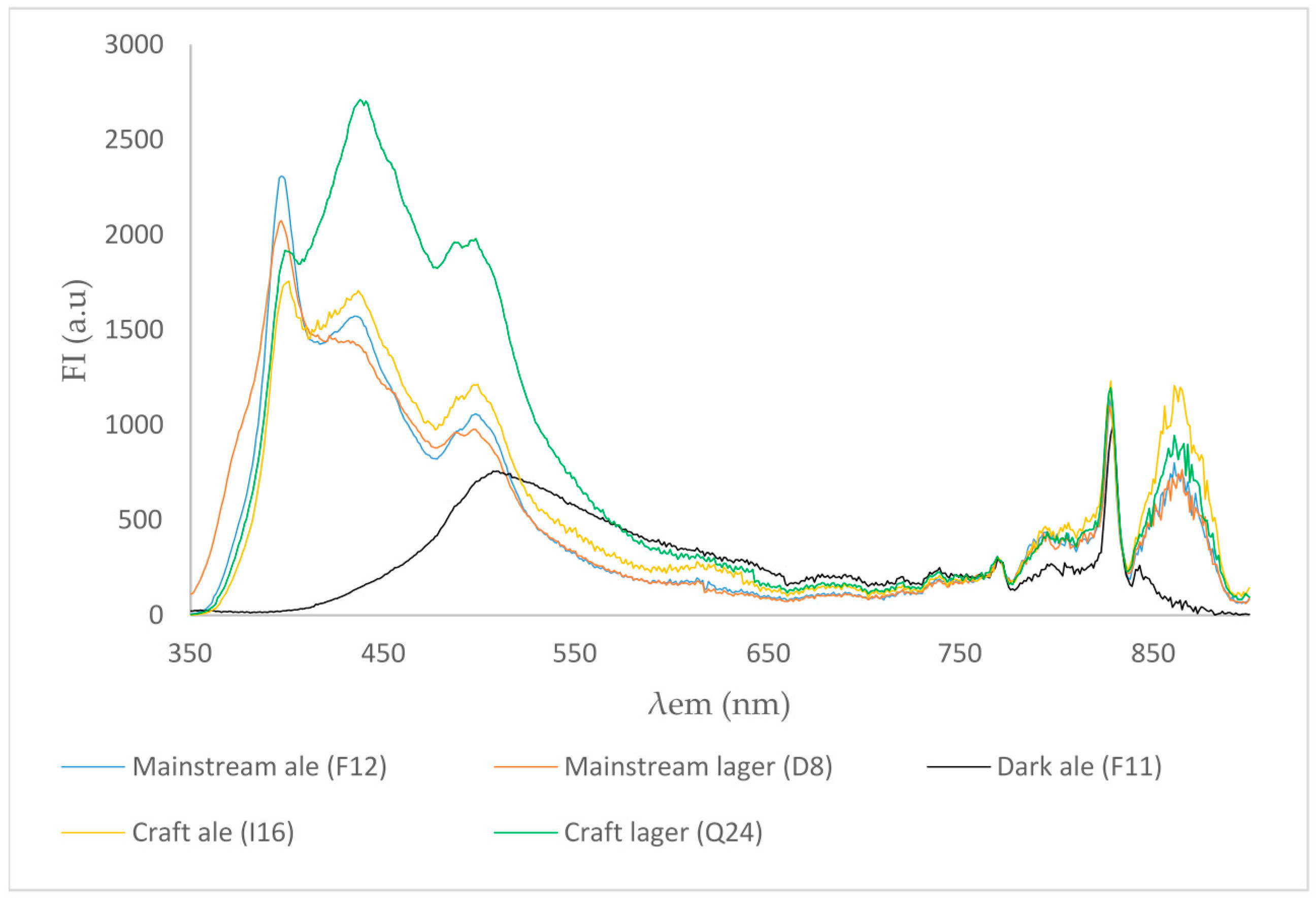
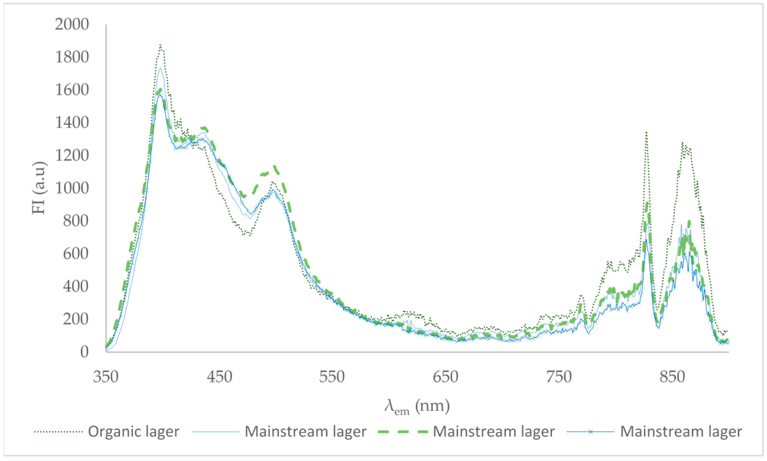
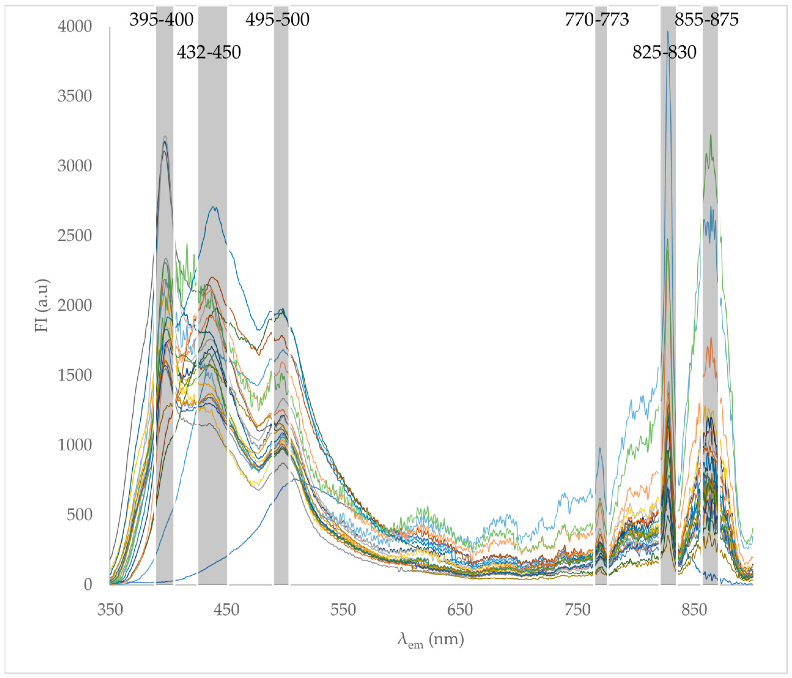
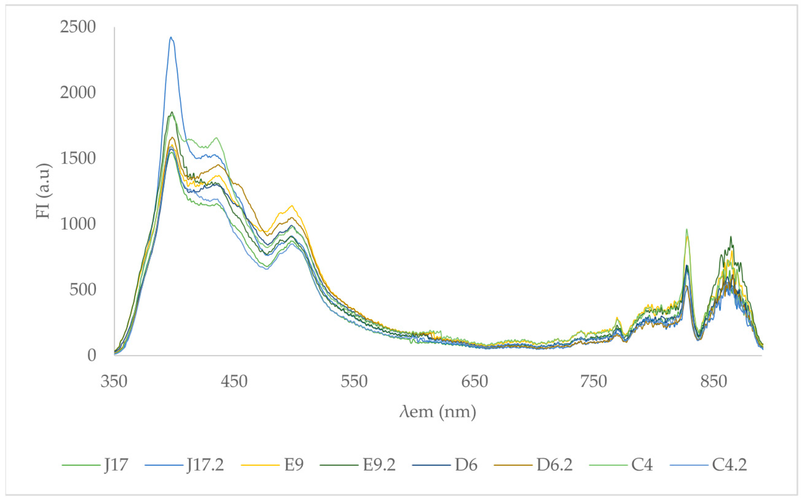
3.1. Synchronous Fluorescence Scan

The synchronous fluorescence spectrum of undiluted, degassed beer samples is shown in Figure 1. Emission intensities varied for each sample. Based on visual interpretation of the peaks, six notable regions were identified and are highlighted in Figure 1. Sample F11 (dark ale) showed a different spectra pattern, compared to the other samples, with shared intensities only at the 770–773 nm and 825–830 nm emission regions.
Emission spectra intensities for beer samples stored for 6 weeks at 4 °C was compared to fresh samples for the respective beer brands (Figure 2). A one-tailed, unequal variance Student’s ‘t’ test was performed on intensity readings between the stored and fresh samples. Significant differences (p < 0.05) were identified at emission intensity regions 395–400, 432–450, 495–500, 770–773, 825–830 nm but not the 855–875 nm region, for the samples displayed in the graph (Figure 2).
Synchronous scanning fluorescence of selected lager beers and ales was compared to show the similarities and differences between these different beer styles (Figure 3). As shown in Figure 3, the dark ale sample had a lower intensity reading and different pattern compared to the other beers.
Lager beer marketed as having organic certification (sample O22) was compared to three different mainstream lager beers (D6, E9 and P23). As shown in Figure 4, the organic beer sample had a higher intensity reading in the 395–400 nm, 825–830 nm (C-H) and 855–875 nm (presumably C-H aromatic groups) regions, compared to the other beers in the figure [14,15,20,21,22].

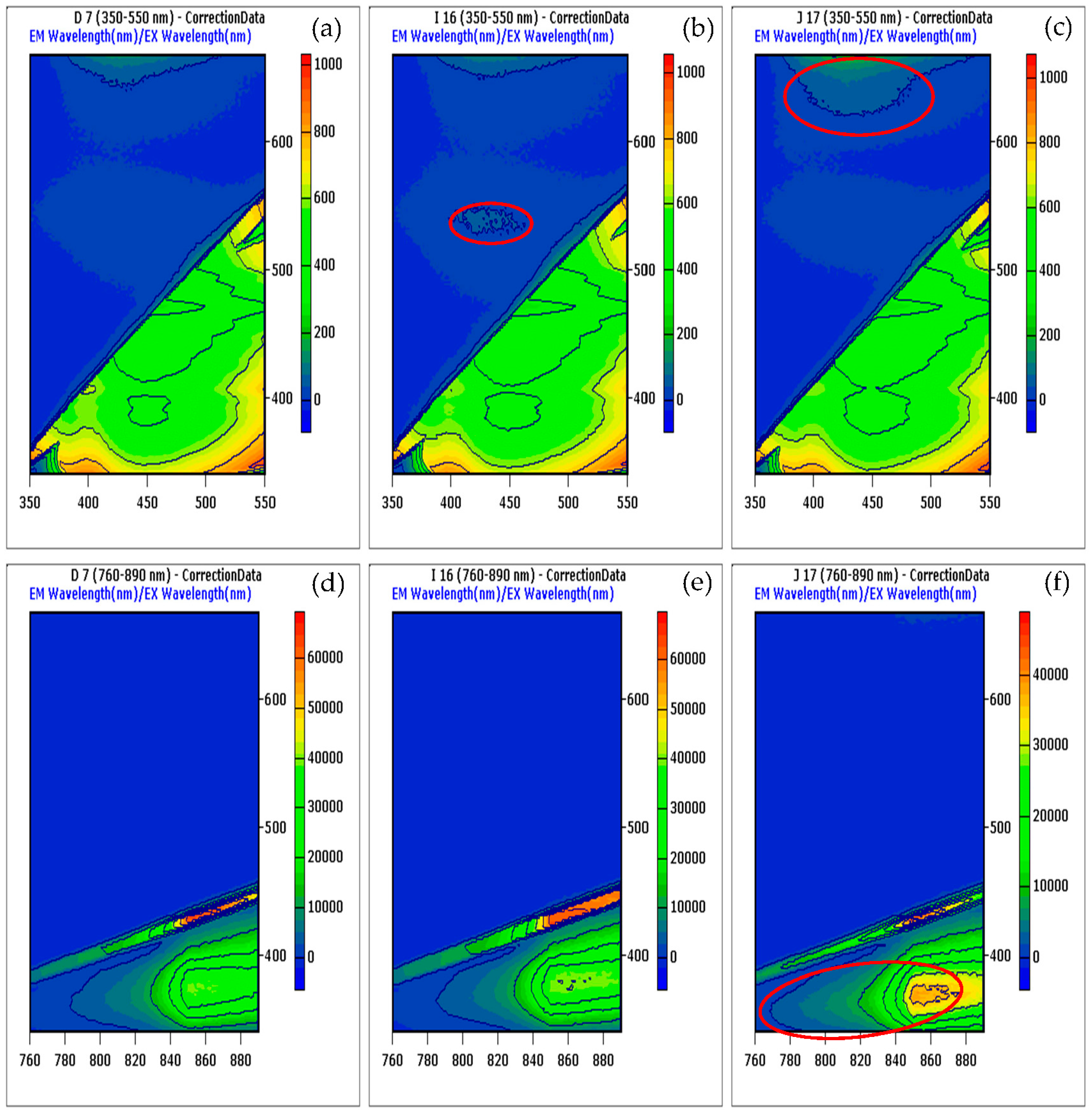
3.2. Emission Excitation Matrix (EEM) Contour Plots

Emission-excitation matrices (EEM) were obtained for some of the beer samples. The analysis involved excitation in the range 340 to 890 nm and two separate scans focusing on the emission range 350 to 550 nm and 760 to 890 nm (Figure 5). Of the three samples analyzed (D7, I16 and J17), there are distinct differences and similarities that can be observed in the EEM contour plots, some of the differences have been circled in red. It is important to note that Rayleigh scattering, which are the diagonal ridges in the contour plots, is a common phenomenon with EEMs and has no relevant information. In the samples analyzed an intense excitation band at about 350 nm and emission at 860 nm (Figure 5d–f) is clearly observed while there is weak intensity at the 430 nm emission and 850 nm excitation region (Figure 5a–c). Emission and excitation at the longer wavelengths (760 to 890 nm) showed less intensity compared to shorter wavelengths [14,15,21,23,24].

4. Discussion

The present paper aimed to use fluorescence spectroscopy to investigate the fluorescence properties of beers manufactured in Australia. Beer is a multicomponent hydroalcoholic solution and therefore the fluorescence characteristics are complex due to overlapping emissions from the numerous species, energy transfer, self-absorption and quenching phenomenon. Nevertheless, the spectra of the matrix provide valuable information about the overall properties of the sample. Based on the results obtained and review of published literature, it is presumed that peaks in the emission range 395–400 nm could relate to iso-alpha acids, 430–450 nm are phenolic compounds, 470–510 are vitamins (e.g., riboflavin) [23] or in the case of dark ales, hydroxymethylfurfural (HMF) [14,15,21,23,24]. Comparing the fluorescence spectra of ales and lagers (Figure 3) shows the dramatic differences between the samples. For the dark ale, noticeable changes appear in the low wavelength region but similarities at long wavelength regions 770–773 nm and 825–830. In the NIR wavelength regions (770–773 nm, 825–830 nm and 855–875 nm) -OH groups or porphyrins derivatives may be the dominant compounds contributing to fluorescence readings [14,15,21,23,24]. Additionally, the O-H bonds, possibly associated with ethanol and phenolic compounds, can be found in this region. As discussed in literature, a fluorophore absorbing in the near infrared region (>700 nm) likely has a low lying excited molecular electronic state which allows electronic transitions at longer wavelengths [21]. It is theorized that the beer samples contain compounds or complexes of molecules (e.g., peptides) that exhibit long-wave length absorption and emission [14,15,21,23,24].
The experiment also tested differences between beers that had been opened and stored at 4 °C for 6 weeks compared to fresh beers. Fluorescence spectroscopy identified that the stored beer was different to the corresponding fresh beer brand. Others have researched storage conditions and found that light exposure was a greater contributing factor than time open for a period of three weeks [15]. In the present study, the differences in fluorescence spectra could be due to evaporation of alcohol or decomposition of the beer as it was stored for a period of 6 weeks. Admittedly, the sample size was small with only four brands analyzed and this result may be casual.
Beer is a complex mixture of chemical components and the 3D contour plots show the differences between each brand (Figure 5). In this example, three different brands were analyzed, while similarities can be identified each plot has distinct differences that can be used to qualitatively differentiate between the brands. It is important to note in the EEMs contour plots light scattering effects such as Raman and Rayleigh scattering are present. The phenomenon usually exists due to a physical process when light passes through samples. For example, first order Rayleigh scattering is identified as the diagonal lines (Figure 5) and these signals carry no relevant information for this experiment [22]. Multiway analysis of fluorescence data (e.g., parallel factor analysis) can be used for analysis of the results and with spectra of known compounds multiway analysis can be used to identify the unknown fluorescent constituents in the beer.

5. Conclusions

In food analysis, spectroscopy is valuable as it provides information about a wide range of different compounds the total sample matrix in a single measurement. To our knowledge, this is the first paper to investigate the fluorescence characteristics of Australian beers in the short and long wavelength regions. Synchronous scanning fluorescence and excitation-emission matrix data showed fluorescence regions that relate to fluorophores commonly found in beer and these regions match with those reported in the literature. The distinct spectra differences identified between dark ales, lagers and craft beers demonstrated that the analysis technique may be used for rapid qualitative classification of beers. Although our sample size consisted of four brands, the impact of storage time was evident with an observable reduction in the emission intensities. Our findings complement other studies that have shown fluorescence spectroscopy can be used to discriminate between undiluted beer samples and that measurements in the long wavelength region can provide additional information about the sample matrix. It is envisioned that a follow up study involving a wider range of Australian produced beverages will be completed in the near future.

Acknowledgments

The study was funded by Central Queensland University.

Author Contributions

R.G. conceived and designed the experiments; R.G. performed the experiments; R.G. analyzed the data; J.C. and D.C. contributed the reagents and materials and have had direction of the preparation and presentation of the manuscript. J.C. provided funding of study, A.P., S.C. and J.J.R. critical review of the manuscript.

Conflicts of Interest

The authors declare no conflict of interest.

References

  1. Australian Bureau of Statistics. Apparent Consumption of Alcohol. Australia, 2015–16; Cat. No. 4307.0.55.001; Australian Bureau of Statistics: Canberra, Australia, 2017.
  2. Argent, N. Heading down to the local? Australian rural development and the evolving spatiality of the craft beer sector. J. Rural Stud. 2017. [Google Scholar] [CrossRef]
  3. Preedy, V.R. Beer in Health and Disease Prevention; Academic Press: Cambridge, MA, USA, 2011. [Google Scholar]
  4. Marconi, O.; Sileoni, V.; Ceccaroni, D.; Perretti, G. The use of rice in brewing. In Advances in International Rice Research; InTech: London, UK, 2017. [Google Scholar]
  5. Bogdan, P.; Kordialik-Bogacka, E. Alternatives to malt in brewing. Trends Food Sci. Technol. 2017, 65, 1–9. [Google Scholar] [CrossRef]
  6. Karoui, R.; Blecker, C. Fluorescence spectroscopy measurement for quality assessment of food systems—A review. Food. Bioprocess Technol. 2011, 4, 364–386. [Google Scholar] [CrossRef]
  7. Bro, R. Exploratory study of sugar production using fluorescence spectroscopy and multi-way analysis. Chemom. Intell. Lab. Syst. 1999, 46, 133–147. [Google Scholar] [CrossRef]
  8. Becker, E.M.; Christensen, J.; Frederiksen, C.S.; Haugaard, V.K. Front-face fluorescence spectroscopy and chemometrics in analysis of yogurt: Rapid analysis of riboflavin. J. Dairy Sci. 2003, 86, 2508–2515. [Google Scholar] [CrossRef]
  9. Christensen, J.; Povlsen, V.T.; Sorensen, J. Application of fluorescence spectroscopy and chemometrics in the evaluation of processed cheese during storage. J. Dairy Sci. 2003, 86, 1101–1107. [Google Scholar] [CrossRef]
  10. Kongbonga, Y.G.M.; Ghalila, H.; Onana, M.B.; Majdi, Y.; Lakhdar, Z.B.; Mezlini, H.; Sevestre-Ghalila, S. Characterization of vegetable oils by fluorescence spectroscopy. Food Nutr. Sci. 2011, 2, 692. [Google Scholar] [CrossRef]
  11. Kyriakidis, N.B.; Skarkalis, P. Fluorescence spectra measurement of olive oil and other vegetable oils. J. AOAC Int. 2000, 83, 1435–1439. [Google Scholar] [PubMed]
  12. Karoui, R.; Dufour, E.; Bosset, J.O.; De Baerdemaeker, J. The use of front face fluorescence spectroscopy to classify the botanical origin of honey samples produced in switzerland. Food Chem. 2007, 101, 314–323. [Google Scholar] [CrossRef]
  13. Tóthová, J.; Žiak, Ľ.; Sádecká, J. Characterization and classification of distilled drinks using total luminescence and synchronous fluorescence spectroscopy. Acta Chim. Slovaca 2008, 1, 265–275. [Google Scholar]
  14. Sikorska, E.; Gorecki, T.; Khmelinskii, I.V.; Sikorski, M.; De Keukeleire, D. Fluorescence spectroscopy for characterization and differentiation of beers. J. Inst. Brew. 2004, 110, 267–275. [Google Scholar] [CrossRef]
  15. Sikorska, E.; Gorecki, T.; Khmelinskii, I.V.; Sikorski, M.; De Keukeleire, D. Monitoring beer during storage by fluorescence spectroscopy. Food Chem. 2006, 96, 632–639. [Google Scholar] [CrossRef]
  16. Insinska-Rak, M.; Sikorska, E.; Czerwinska, I.; Kruzinska, A.; Nowacka, G.; Sikorski, M. Fluorescence spectroscopy for analysis of beer. Pol. J. Food Nutr. Sci. 2007, 57, 239–243. [Google Scholar]
  17. Tan, J.; Li, R.; Jiang, Z.T. Chemometric classification of chinese lager beers according to manufacturer based on data fusion of fluorescence, uv and visible spectroscopies. Food Chem. 2015, 184, 30–36. [Google Scholar] [CrossRef] [PubMed]
  18. Apperson, K.; Leiper, K.A.; McKeown, I.P.; Birch, D.J. Beer fluorescence and the isolation, characterisation and silica adsorption of haze-active beer proteins. J. Inst. Brew. 2002, 108, 193–199. [Google Scholar] [CrossRef]
  19. Dreve, S.; Voica, C.; Dragan, F.; Georgiu, M. Instrumental Analysis for Differentiation of Beers and Evaluation of Beer Ageing. AIP Conf. Proc. 2013, 290–293. [Google Scholar] [CrossRef]
  20. Christensen, J.; Norgaard, L.; Bro, R.; Engelsen, S.B. Multivariate autofluorescence of intact food systems. Chem. Rev. 2006, 106, 1979–1994. [Google Scholar] [CrossRef] [PubMed]
  21. Sauer, M.; Hofkens, J.; Enderlein, J. Handbook of Fluorescence Spectroscopy and Imaging; Wiley-VCH Verlag GmbH & Co. KGaA: Weinheim, Germany, 2011; pp. I–IX. [Google Scholar]
  22. Engelen, S.; Moller, S.F.; Hubert, M. Automatically identifying scatter in fluorescence data using robust techniques. Chemom. Intell. Lab. Syst. 2007, 86, 35–51. [Google Scholar] [CrossRef]
  23. Sikorska, E.; Gliszczynska-Swiglo, A.; Insinska-Rak, M.; Khmelinskii, I.; De Keukeleire, D.; Sikorski, M. Simultaneous analysis of riboflavin and aromatic amino acids in beer using fluorescence and multivariate calibration methods. Anal. Chim. Acta 2008, 613, 207–217. [Google Scholar] [CrossRef] [PubMed]
  24. Sikorska, E.; Khmelinskii, I.; Sikorski, M. Fluorescence methods for analysis of beer. In Beer in Health and Disease Prevention; Elsevier: Amsterdam, The Netherlands, 2009. [Google Scholar]
Figure 1. Emission spectra for all freshly opened beer samples (1–24). The six shaded areas indicate regions of varying intensity that are believed to be specific to the fluorophore compounds in beer and therefore can be used to differentiate between beer samples.
Beverages 03 00057 g001
Figure 2. The emission spectra between for stored and fresh beer samples (J17 vs. J17.2, E9 vs. E9.2, D9 vs. D9.2 and C6 vs. C6.2).
Beverages 03 00057 g002
Figure 3. Synchronous scanning fluorescence spectra of select beers showing the differences between a dark ale (F11), craft ales (I16), mainstream ales (F12), craft lagers (Q24) and mainstream lagers (D8).
Beverages 03 00057 g003
Figure 4. The emission spectra of select beers showing the differences between the organic lager (O22) and mainstream lager beers (D6, E9 and P23).
Beverages 03 00057 g004
Figure 5. Contour map of the emission excitation matrix (EEM) of select beer samples (D7, I16 and J17). The color bar ranging from low (blue) to high (red) shows the signal intensity for each sample is shown. (a) Sample D7 at emission range 350 to 550 nm and excitation range from 340 to 890 nm; (b) sample I16 at emission range 350 to 550 nm and excitation range from 340 to 890 nm; (c) J17 at emission range 350 to 550 nm and excitation range from 340 to 890 nm; (d) at emission range 350 to 550 nm and excitation range from 340 to 890 nm; (e) Sample I16 at emission range 760 to 890 nm and excitation range from 340 to 890 nm; (f) sample J17 at emission range 760 to 890 nm and excitation range from 340 to 890 nm.
Beverages 03 00057 g005
Table 1. List of the beer samples analyzed in this study.
Beer Manufacturer 1Sample Name 2ABV (%) 2IBU 2Style 2
A14.514Craft Lager
B24.840Craft Ale
C33.522Helles
C44.218Craft Lager
C4.24.218Craft Lager
C5518Wheat beer
D64.925Lager
D6.24.925Lager
D74.923Lager
D83.525Lager
E93.515Lager
E9.23.515Lager
E104.419Lager
F114.5-Dark ale
F123.5-Pale ale
G134.525Craft Ale
H143.5-Lager
H150.9-Lager
I164.527Craft Ale
J17516Lager
J17.2516Lager
K184.2-Craft Ale
L194.520Ale
M205.934Lager
N214.515Wheat beer
O224.6-Lager
P234.617Lager
Q244.932Craft
1 Letters A-Q refer to the beer manufacturer. Beer brands were assigned a number 1–24. Samples 4.2, 6.2, 9.2 and 17.2 were opened and stored for 6 weeks prior to analysis. 2 Alcohol by volume (ABV %), international bitterness units (IBU) and beer style information as reported by the manufacturer.

