
Hydrodynamic Modeling of Nokoué Lake in Benin

1
Laboratory of Applied Hydrology, University of Abomey-Calavi, 229 Cotonou, Benin
2
Laboratory of Modeling in Hydraulics and Environment, University of Tunis El Manar, 1002 Tunis, Tunisia
*
Author to whom correspondence should be addressed.
Hydrology 2016, 3(4), 44; https://doi.org/10.3390/hydrology3040044
Submission received: 1 May 2016
/
Revised: 3 December 2016
/
Accepted: 6 December 2016
/
Published: 15 December 2016
(This article belongs to the Special Issue Floods and Landslide Prediction)
Abstract
:Nokoué Lake is a complex ecosystem, the understanding of which requires control of physical processes that have occurred. For this, the Surface Water Modeling System (SMS) hydrodynamic model was calibrated and validated on the water depth data. The results of these simulations show a good match between the simulated and observed data for bottom roughness and turbulent exchange coefficients, of 0.02 m−1/3·s and 20 m2/s respectively. Once the ability of the model to simulate the hydrodynamics of the lake is testified, the model is used to simulate water surface elevation, exchanged flows and velocities. The simulation shows that the tidal amplitude is maximum at the inlet of the channel and decreases gradually from the inlet towards the lagoon’s main body. The propagation of the tidal wave is characterized by the dephasing and the flattening of the amplitude tide, which increases as we move away from the channel. This dephasing is characterized by a high and low tides delay of about 1 or 4 h and also depends on the tide amplitude and location. The velocities inside the lake are very low and do not exceed 0.03 m/s. The highest are obtained at the entrance of the channel. In a flood period, in contrast with the low-water period, incoming flows are higher than outflows, reinforced by the amplitude of the tide. An average renewal time of the lake has been estimated and corresponds during a flood period to 30 days for an average amplitude tide and 26.3 days on a high amplitude tide. In a low water period it is 40.2 days for an average amplitude tide and 30 days for a high amplitude tide. From the results obtained, several measures must be taken into account for the rational management of the lake water resources. These include a dam construction at the lake upstream, to control the river flows, and the dredging of the channel to facilitate exchanges with the sea.
1. Introduction
Coastal lagoons are by nature complex and fragile systems characterized by large fluctuations in the physical and chemical parameters. Over the last decades, they have also become an extremely valuable, due to the enormous potential for residential, tourism, economic (mainly, shellfish/fish farming), and recreational development [1]. However, due to global warming, reduced river flows and rising sea levels, these aquatic ecosystems are increasingly vulnerable and threatened by eutrophication [2,3,4,5]. The preservation of the natural abilities of these environments, while ensuring better management and exploitation of these lagoon environments, requires a good knowledge of the hydrodynamic processes that take place there. Indeed, the movement of water masses in a lagoon environment results mainly from the friction exerted by the wind on the surface of the water body and variations in sea level. Locally, the rivers that join the lagoon modify the dynamics in the zone near their mouth. Conversely, the dissipation of energy by friction on the bottom of the lagoon limits the movements of the water body [6].
The object of this study, Nokoué Lake, is a complex ecosystem, the understanding of which requires the mastery of the physical processes that occur in the basin; the most important of these is hydrodynamics. Several forcing mechanisms such as wind, astronomical tide and river discharges are simultaneously acting in the lake.
Thus, knowing the lake reaction in face of natural and anthropogenic forcing has become a major issue. For this, beyond a descriptive approach, it is appropriate to develop predetermination and the general functioning of lake simulation tools, which obviously requires the prior construction of a hydrodynamic model [7]. In fact, hydrodynamic models are used to quantify sea water inflow volumes and predict hydraulic parameters (e.g., water velocity in the lagoon mouth). It is also necessary to make better decisions with regard to lagoon restoration design and management actions for improvement of environmental conditions. Indeed, important exchanges with the marine environment will favor the export and dilution of contaminants, nutrients and pollutants, while limited trade with the sea may result in an accumulation of contaminants and nutrients in the lagoon, making it more vulnerable [8].
Several studies have examined the hydrodynamic functioning of lagoons in Africa using numerical models [9,10,11,12,13]. They have allowed us to analyze processes such as distribution of water levels, currents and flushing rates that takes place in lagoons. The description of these different processes at Nokoué Lake requires the use of a 2D numerical model as a support for understanding the hydrodynamic functioning. The purpose of this paper is therefore to understand the mechanism of water circulation in the lake.
2. Materials and Methods
2.1. Study Area
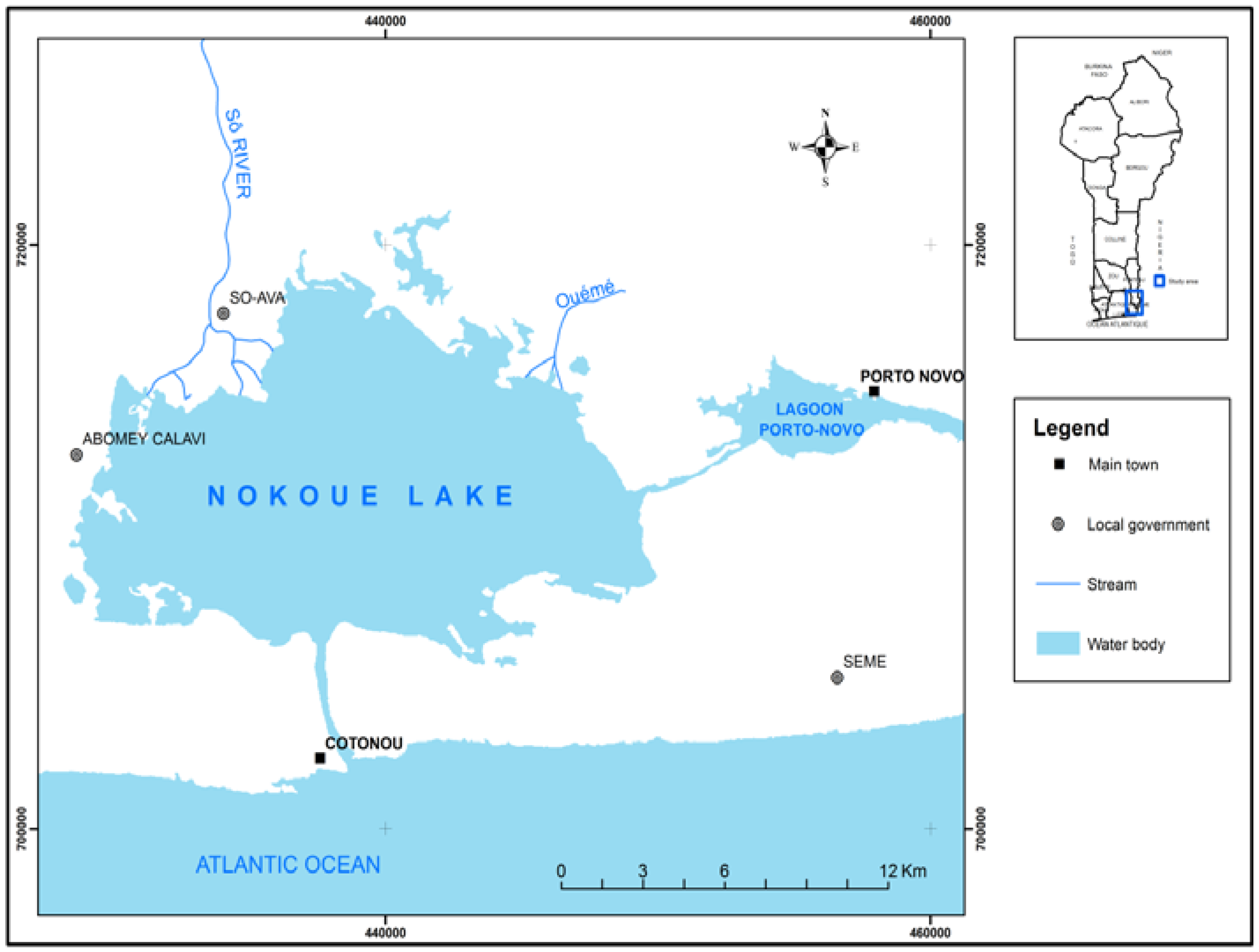
Nokoué Lake, the largest area of brackish waters of Benin (150 km2) and one of the largest West African lagoons, is located in the south of Benin, between 6°25′ N and 2°36′ E (Figure 1). It is characterized by a subtropical climate, and undergoes two rainy seasons and two dry seasons of unequal duration. The average annual rainfall is 1309 mm, the average temperature of 27.7 °C, with maximums up to 33 °C and minimums at 23 °C.
The lake is connected to the lagoon of Porto-Novo in the East by Totche channel, to the Atlantic Ocean at south by Cotonou channel, and in the north it receives the Sô River and Ouémé stream. According to the typology of the lagoons [14], it is a partially enclosed lagoon while being in constant communication with the ocean. This communication, combined with the effect of natural flood of Ouémé stream and Sô River, causes significant seasonal variations in salinity [15].
2.2. SMS Model Presentation
A Surface Water Modeling System (SMS) is developed by the Environmental Modeling Research Laboratory (EMRL), at Brigham Young University. SMS is a model well suited to large areas with very complex geometry that are however shallow and unlaminated, such as Nokoué Lake. It is a two-dimensional model using the finite element method to solve the equations of local mass balance and momentum built over the water level [7]. It computes water surface elevations and horizontal velocity components for subcritical, free-surface two-dimensional flow fields [16]. For our study, we use the version 10 of the SMS software, which additionally includes preprocessor modules for meshing and postprocessing interface for analysis.
The three basic equations 2D, resolved by the software in an orthogonal coordinate system (O, x, y) are the following:
Equation of continuity:
Momentum equation on the axe Ox:
Momentum equation on the axe Oy:
where h is the water depth (m), u and v velocities (m/s) in the cartesian directions, x, y, t Cartesian coordinates and time, x and y are the Cartesian coordinates describing the two directions of the plane (m), ρ is the density of water (kg·m3), ρa is the density of air (kg·m3), m0 represents trade surface water (rain, evaporation) or the bottom (infiltration) (m·s−1), Eij are the eddy viscosity coefficients (or dispersion) (m2·s−1), g is the acceleration due to gravity (m·s−2), a is the dimension of the base (m), n is the Manning coefficient reflecting bottom roughness (m−1/3·s), ζ is the coefficient of friction due to wind, Va is the module of the wind speed (m·s−1), φ is the wind direction relative to the axis Ox (rd), ω is the Rate of earth’s angular rotation (rd·s−1), and φ is the site latitude (°).
Equations (1) to (3) are supplemented by boundary conditions of the domain: zero flow (closed borders), imposed water level (open boundary), and imposed flow (corresponding to the rejection of a factory or electric power station). These equations where the unknowns are u, v, and h, do not admit analytic solutions. They are then solved numerically using the finite element method, and time derivatives are replaced with approximations to nonlinear finite differences. The solution is fully implicit and the non-linear equations of the flow are solved simultaneously by the iterative method of Newton-Raphson [7,16].
2.3. Model Building
Construction of a hydrodynamic model consists of introducing the geometry of the area, to discretize the physical space (Lake Mesh), to define the initial and boundary conditions (closed borders, places of exchange and communication with the sea).
2.3.1. Discretization of the Physical Space
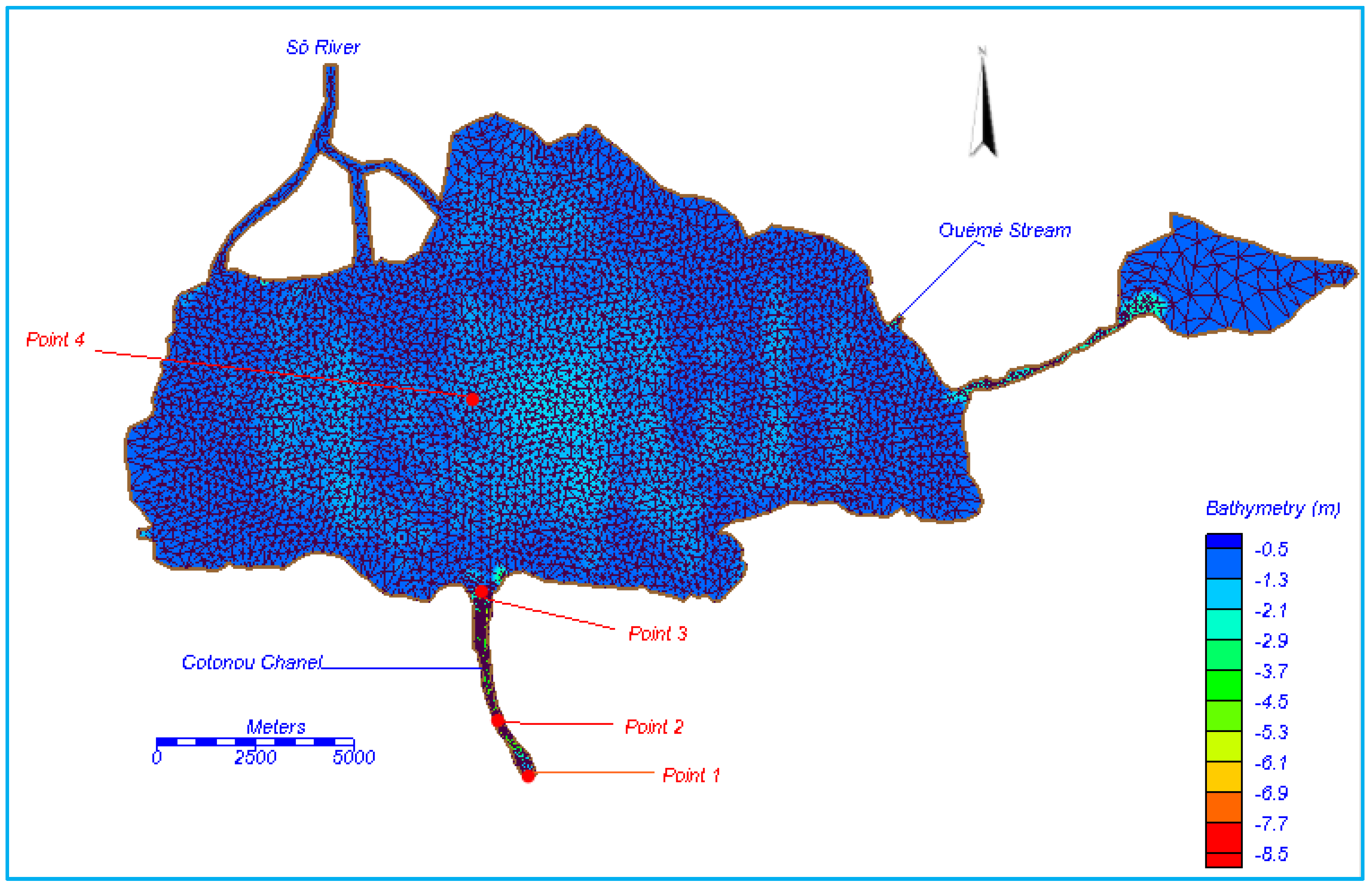
Figure 2 shows that the lagoon is shallow, with a bathymetry between 1 and 2 m. The high depths are found at Cotonou channel with values up to 5 m. The depth of the Totche channel is around 2.5 m.
The data we use are from bathymetric surveys conducted by the General Direction of Water in 2013 and 2014.
From bathymetric data and the lake contour file obtained from the General Direction of Water (DGEau), we made a discretization of the field in 7801 triangular quadratic elements by 6 nodes, and obtain 16,238 nodes (Figure 2). The mesh has deliberately been refined in communications where the side of the elements does not exceed 25 m. The side elements exceed 100 m inside the lake.
Four points have been positioned on the Lake (Figure 2) to analyze the amplification and the phase shift of the tidal wave as it propagates in the lake. Point 1 is selected at the entrance of the Cotonou channel, in it communication with the sea, the point 2 in the channel, at the measuring station of the General Direction of Water, the point 3 at the entrance of Cotonou channel in the lake, and point 4 at the center of the lake.
2.3.2. Boundary and Initial Conditions
The initial state of the area is such that all speeds (horizontal currents) are set to zero everywhere in the field. Thus, in the initial state, the system is assumed uniformly stationary (motionless) and have horizontal level of the free surface of the water [16].
The computational time interval should be small enough to capture the extremes of the dynamic boundary conditions and maintain numerical stability. For this, we retain 0.5 h time step for our simulation.
The first 24 h of simulation are not considered because they represent the spin-up time of the model, necessary to reach a dynamic steady state.
Three types of conditions are used in our study:
The Condition at the Upstream Limit: the Lake Tributaries Flows
Due to a lack of data on the lake inlets, we estimated the inflows from Bonou station, located in the lake upstream, and that feeding the Sô River and Ouémé stream. The initialization phase of the model was established by constant flow simulations, because there was no significant variation in flow during selected periods.
The Sô River flows were estimated from historical values of rate at Bonou and Sô Ava stations by using the linear regression equation obtained with determination coefficient equal to 0.7.
With Y corresponding to Sô flow and X to Bonou flow (in m3/s).
After making flow measurements at Bonou station and Ouémé entry in the lake, Mama, 2010 [17] estimated at 30% the proportion that enters in the lake. Based on this, we calculated from Bonou rates the flow that enters in the lake by Ouémé.
The Flow data were obtained at DGEau. Data from rating curves obtained from the gauging made by a bottom mounted Acoustic Doppler Current Profiler (ADCP).
The Boundary Condition at the Downstream: The Tide
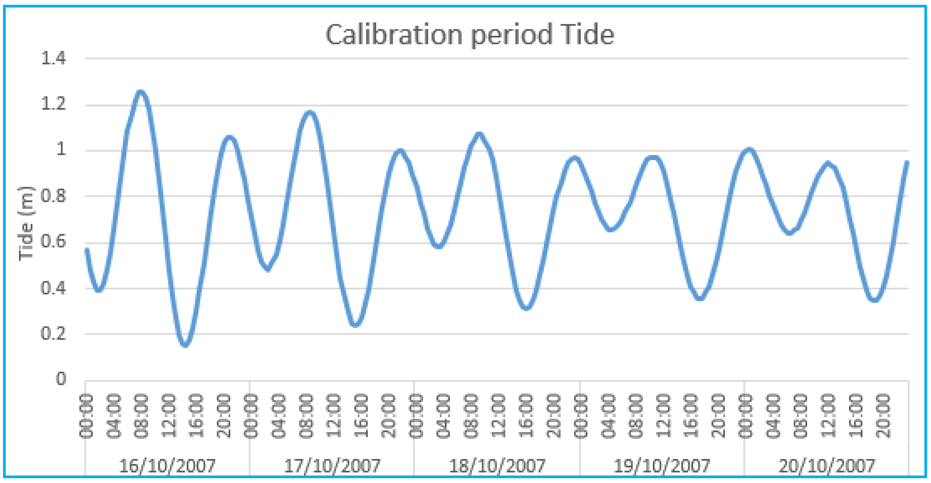
The tide data (hourly) are extracted from WXTide32 software freely available on Internet and cover the periods shown in Table 1. Figure 3 show the tide of calibration period.
The curve indicates a semi-diurnal tide with diurnal inequality. The average over the period is 0.72 m with an amplitude of 1.1 m. The tide level has varied between a maximum of 1.25 m in high tide and 0.15 m in low tide.
Condition at Upper Limit: Wind, Precipitation, and Evaporation
The first climatic parameter considered is the wind. In fact, SMS provides the capability to include storm fronts in simulation. This is accomplished by generating spatial variations in wind speed and direction for each time step. For this we used RMA2 Original Formula.
where Va is the wind speed (in m/s), θ is the angle of the wind relative to OX axis (pointing to east), τSX and τSY are the shear components generated in surface (g/m·s2) on the x axis (pointing to east) and Y axis (pointing to north).
Hourly wind speed and direction have been obtained on Free Meteo website (http://freemeteo.co.uk) and cover the periods shown in Table 1. In addition, hourly wind speed and direction are taken from a meteorological station located at 4.3 km from Cotonou (Latitude 6.350; Longitude 2.383 and Altitude of 53 m).
The prevailing wind direction is North East and varies between 7.2 and 1.94 m/s.
Other climatic parameters taken into account by the model are rainfall and evaporation. The input variable of these parameters in the model is such that we have to subtract the average evaporation from the average precipitation to get the value.
For this, the average rainfall and evaporation at Cotonou for each period (Table 1) were taken into account. These data were obtained at the Agency for the Safety of Air Navigation in Africa (ASECNA) and are from the meteorological station of Cotonou airport.
2.4. Calibration Parameters
The calibration of a model is done by qualitative comparison of short time series of water depth produced by the numerical model with field data for the same place and the same period [18,19]. The model’s different data (tide, flow rates, velocity and wind direction) are imposed simultaneously.
Like any hydrodynamic model, the SMS model requires the introduction of some parameters which are generally determined by calibration. In particular, it consists of the determination of:
- -
- The Manning roughness coefficient of the bottom (n), which translated the bottom friction;
- -
- The turbulent exchange coefficient (Eij), which reflects the turbulence and dispersion phenomena due to non-uniformity of velocity along the water level.
In general, in natural environments, the value of Manning coefficient varies between 0.02 to 0.1 m−1/3·s, while the turbulent exchange coefficient, for shallow depths ecosystem from 1 to 20 m2/s [7]. The determination of these parameters is done by adjusting (or sensitivity test) until obtaining field data [19,20].
2.5. Model Performance Evaluation
In order to calibrate and validate the models and for comparison purposes, some quantitative information is required to measure model performance.
2.5.1. The Root Mean Square Error (RMSE)
Also called the root mean square deviation (RMSD), it is a frequently used measure of the difference between values predicted by a model and the values actually observed from the environment that is being modelled. The RMSE of a model prediction with respect to the estimated variable Xmod is defined as the square root of the mean squared error:
where Xobs is observed values and Xmod is modelled values at time/place i.
2.5.2. Coefficient of Determination R2
The coefficient of determination is a statistical measure of how well the regression line approximates the real data points.
2.5.3. Correlation Coefficient, r
It indicates the strength and direction of a linear relationship between two variables (for example model output and observed values). It is obtained by dividing the covariance of the two variables by the product of their standard deviations.
With n serie of the variable, the mean of the observed data, xi observed data, the mean of the predicted data, yi predicted data.
2.5.4. Nash-Sutcliffe Model Efficiency Coefficient (NSE)
The Nash-Sutcliffe model efficiency coefficient (NSE) is commonly used to assess the predictive power of hydrological discharge models [21].
where Xobs is observed values, Xmod is modelled values and observed mean.
3. Results and Discussion
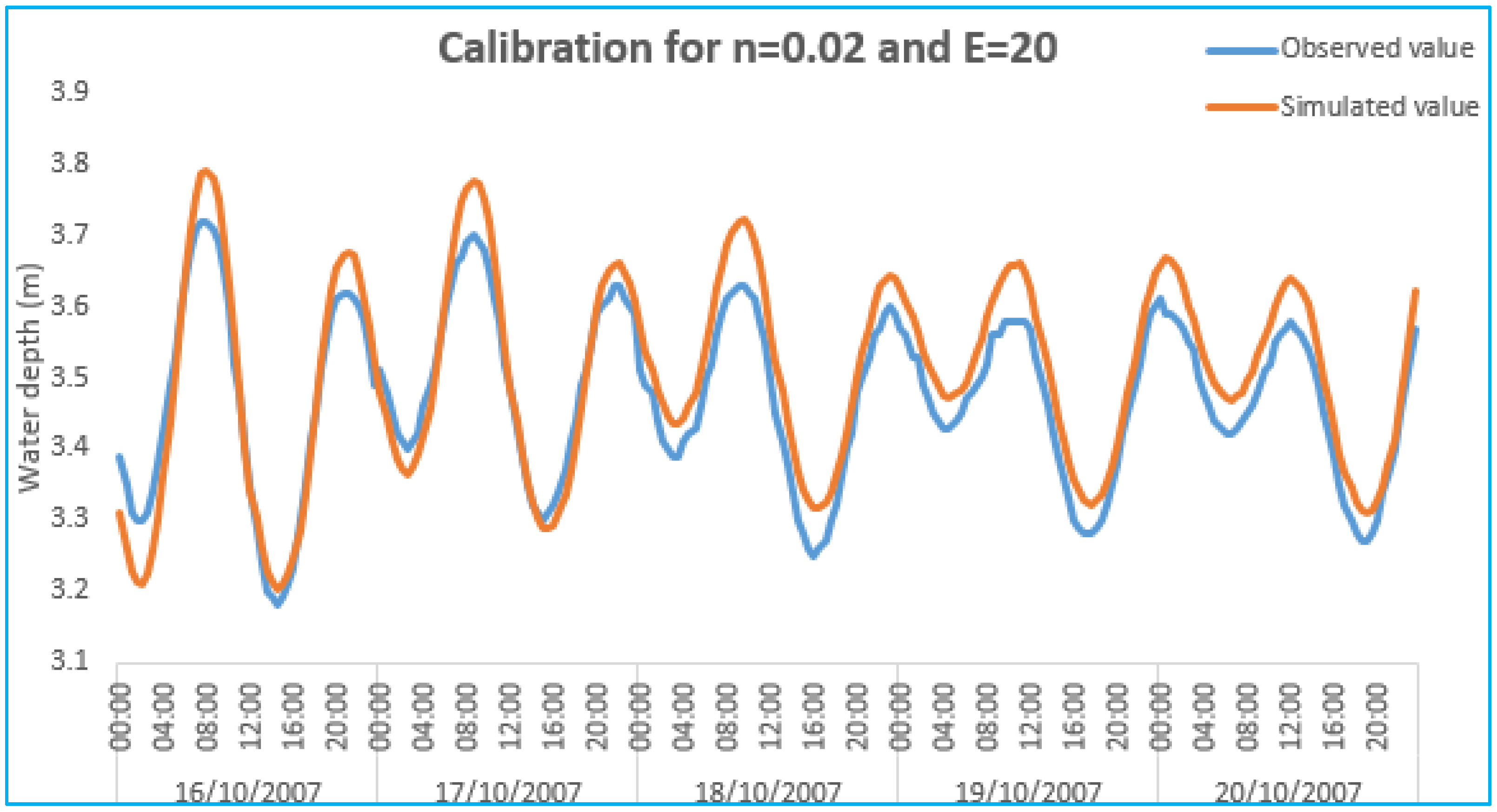
3.1. Model Calibration
Sensitivity tests were initially carried out in order to analyze the hydrodynamic model sensitivity to the variations in the initialization parameters.
We then performed simulations with different values of bottom roughness coefficient (especially n = 0.02; 0.03 and 0.05 m−1/3·s) and different values of the turbulent exchange coefficient (E = 5; 10; and 20 m2/s), that are supposed to be isotropic. For each pair of parameters, the model performance evaluation criteria were applied by comparing water levels measured to those simulated in point 2, located in the Cotonou channel at the measuring station of the General Direction of Water (Figure 2). The objective of this sensitivity test is to find the coefficient values that allow to approach field measurements (water depth).
From the various tests performed, we can notice that among the three cases of roughness tested, the coefficient corresponding to 0.02 m−1/3·s provides the most acceptable performance criteria. It is about 0.97 for correlation coefficient, and 0.87 for determination coefficient. This coefficient is close to the one proposed by [22] in the hydrodynamic modeling of Portugal lagoon. According to them the value of the coefficient of roughness is proportional to the water depth. Thus, for a depth between 3 and 10 m, the value of n corresponds to 0.018.
Among the three turbulent exchange coefficient values tested, the case which equals to 20 m2/s indicates the highest performance criteria demonstrated by NSE value which equal to 84%.
This value is larger than the one calculated for a small sheltered lake (0.005–0.025 m2/s) [23] and similar to those about coastal waters, which are typically between 0.2 and 30 m2/s [24]. However, it is greater than those observed by [20] in the hydrodynamic modeling of systems Aby and Ébrié in Ivory Coast.
Figure 4 shows the curve of evolution of the simulated water depth and observed at point 2 for a simulation of 120 h.
From the analysis of this figure, we can note that the model reproduces the general shape of the observed data, in particular the high and low tide. This is evidenced by the high value of the coefficient of correlation and determination. Also, we should note that the model slightly overestimates both the high tide and the low tide. The performance indicator RMSE applied to the series indicates a value equal to 0.05 m.
It is therefore obvious that the model reproduces fairly well the pace of field data variation, but do not fully reflect the magnitude of changes.
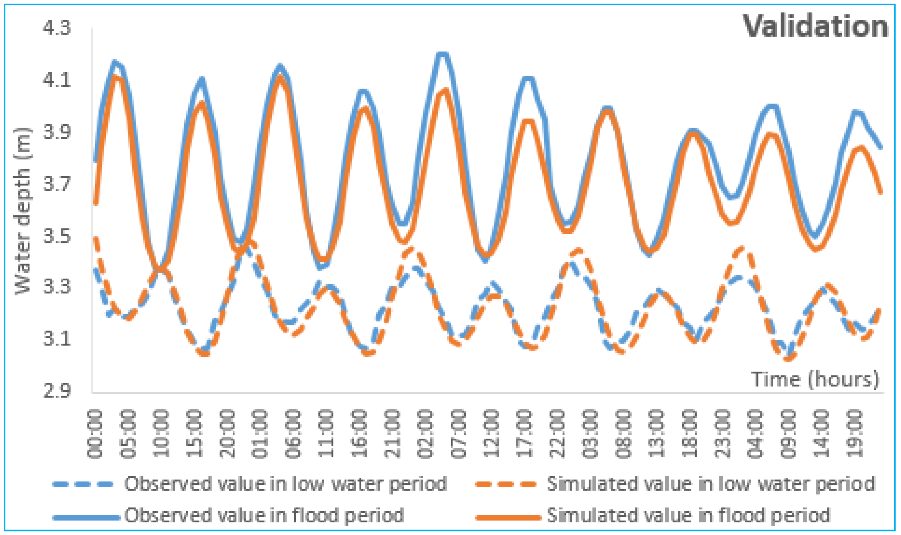
3.2. Validation
After the model was calibrated, we tried to validate it. For this, two periods were retained, particularly from 16 to 20 October 2008 for flood period and 19 to 23 December 2008 for low water period.
From the analysis of the Figure 5, we notice that water depths values observed and simulated are highly correlated. It is testified by the values of correlation coefficients that are respectively 0.97 for the flood period and 0.93 for the low water period. The values of determination coefficients are 0.95 for the flood period and 0.87 for the low water period, while those of NSE indicate respectively 0.64 and 0.73 for the flood and low water period.
The model reproduces perfectly both periods of high and low tide, but overestimates water depths. This testifies the RMSE values that are respectively 0.094 and 0.034 m for the flood period and the low water period. This difference could be explained by the fact that the period of bathymetry is recent to validation period. Also, the model did not take into account exchanges with Porto Novo lagoon, due to lack of observations for the latter.
Overall the defects seem minor and are not of a nature to jeopardize the ability of the model to reproduce the hydrodynamics of Nokoué Lake.
Thus, the level of agreement between prediction and the observed values of water depth allows to verify that the model is able to simulate satisfactorily the hydrodynamic behavior of the lake and it can therefore be used for long term simulation.
3.3. Hydrodynamic Functioning of the Lake
Once the model is built, calibrated and validated, we can use it to perform simulations, including the study of the hydrodynamics of the lake. For the analysis the period from 15 September to 15 October 2014 corresponding to the flood period and the period from 1 to 31 January 2015 corresponding to the low water period were retained. To accurately observe the temporal and spatial variation of water surface levels, flow and distribution of the velocity field, we considered a 24 h simulation period (Table 2).
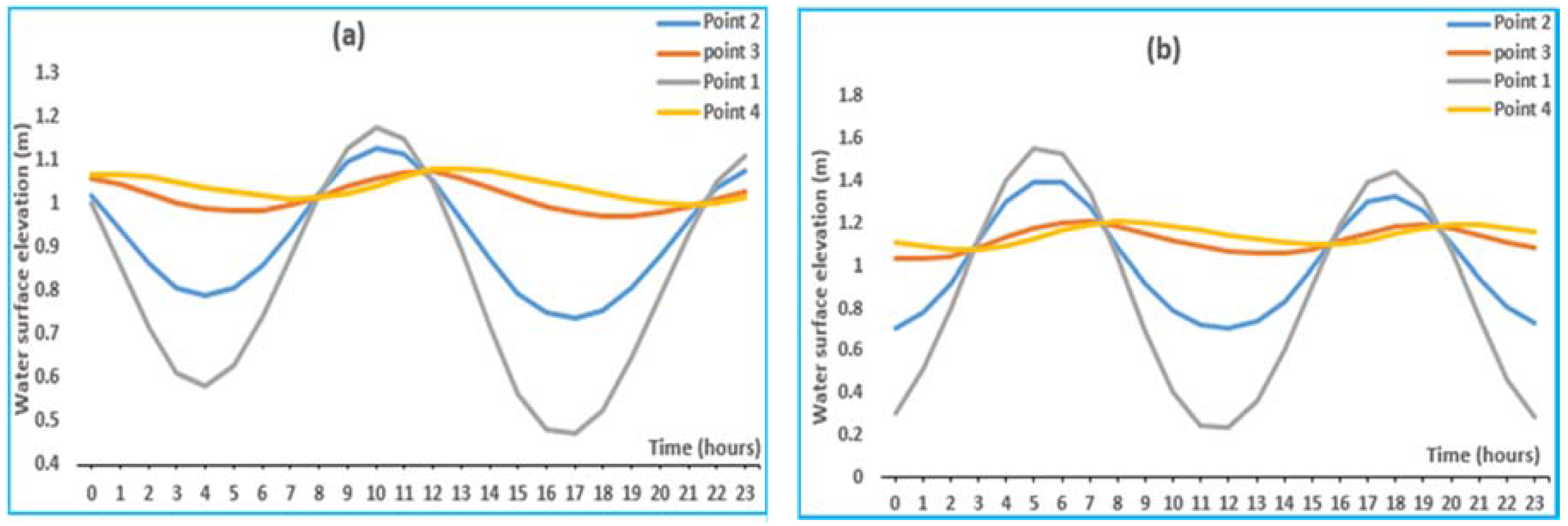
3.3.1. Variation of the Water Surface Level
Figure 6a,b respectively show the variations of the water surface elevation in average and high tidal amplitude during a flood period.
The variation of the water surface at the points 1 and 2 follows the same pattern and may be decomposed at point 1 in four phases:
From 0 h to 4 h, we have the reflux, period during which the water surface drops to 0.58 m. From 4 h to 10 h: it is the flow, the level of the water surface rises to 1.17 m. From 10 h the level of the water surface drops to 0.47 m at 17 h. After 17 h there is a recovery.
From point 1 to point 4, there is a decrease in tidal amplitude going from 0.7 m to 0.3 m at point 2. At point 3 this drop corresponds to 0.6 m with a delay of 1 h for low tide and 2 h for high tide. At point 4, there was a decrease of approximately 0.61 m with a 4 h delay in low tide and 3 h for high tide.
At Figure 6b, there is a gradual decline of the tidal amplitude from 1.32 m at point 1 to 0.14 m at point 4. We observe in point 3 a dephasing about 1 h and 2 h respectively during low and high tide periods. While at point 4, it is about 4 and 3 h respectively in low and high tide periods.
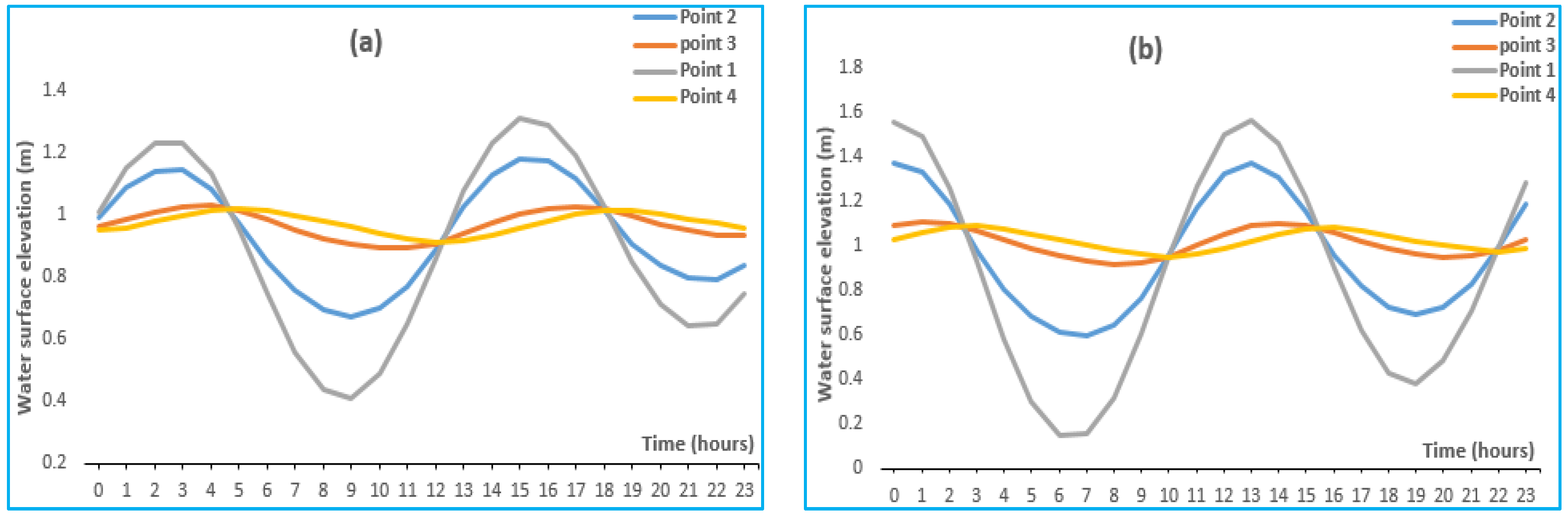
Figure 7a,b show the variations of the water surface in average and high tidal amplitude during a low water period. From the analysis of Figure 7a, the water surface change at points 1 and 2, follows the same trend and can be decomposed as follows in point 2.
From 0 h to 7 h, it is the reflux, corresponds to the descent of the level of the surface of the water to 0.15 m. It follows from 7 h to 13 h by a rise of the water surface, reaching the highest level of 1.57 m. From 13 h, the level of the water surface drops and reach the value of 0.37 m at 19 h. After 19 h, there was a rise in the level of the water surface.
From point 1 to point 4, there is a gradual decline of the tidal amplitude from 0.9 m to 0.51 m in point 2. In point 3 this drop corresponds to 0.76 m with a delay of 2 h for low tide and 1 h for high tide. At point 4, there was approximately a decrease of 0.78 m with 3 h delay in low tide and 2 h for high tide.
Figure 7b shows a gradual decline in the amplitude of the tide from 1.42 m in point 1 to 0.14 m in point 4. We observe in point 3 a dephasing of about 2 h and 1 h respectively during periods of low and high tide. While at point 4, it is about 4 h and 3 h respectively in low and high tide periods.
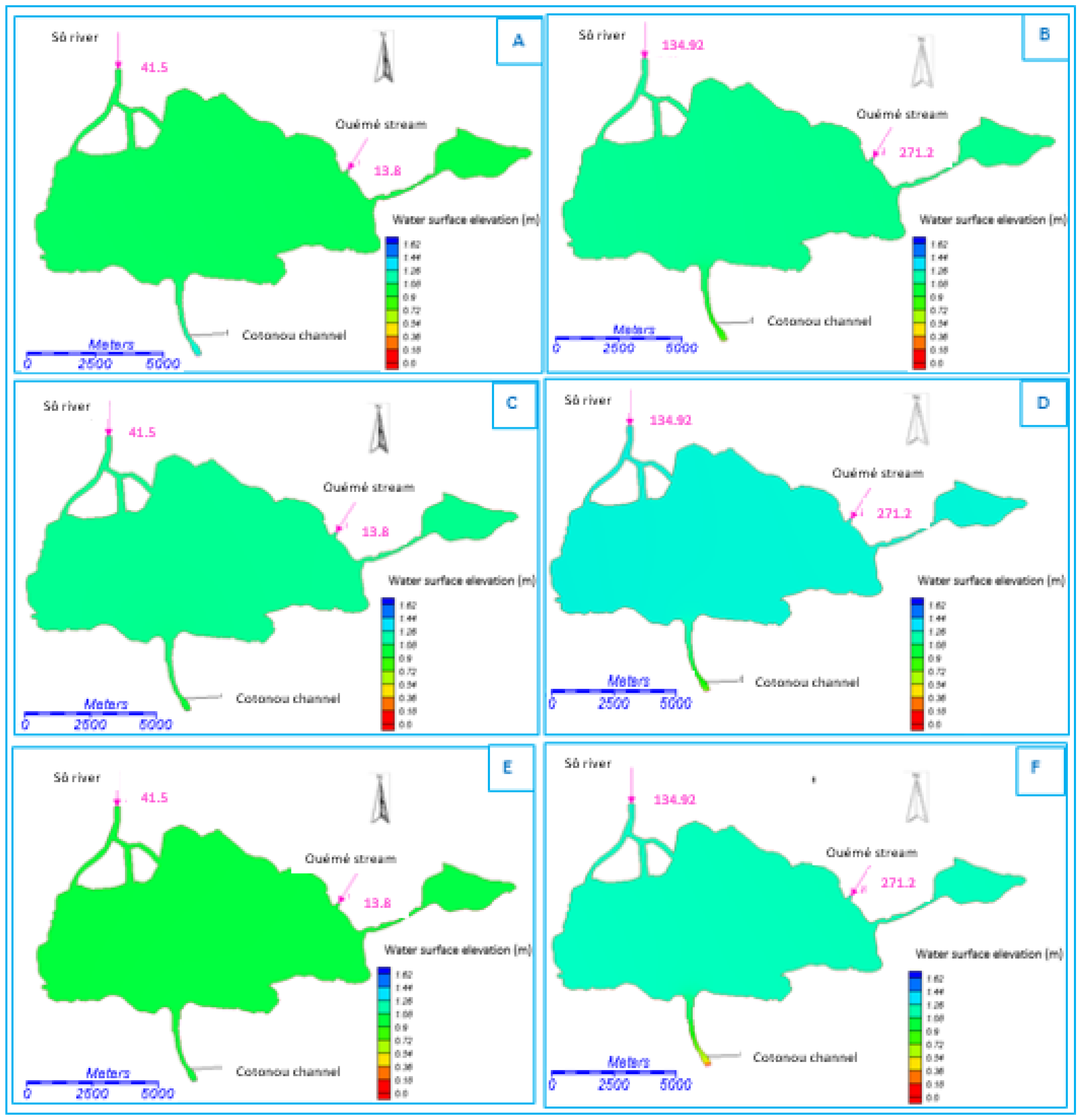
Figure 8 (graph A to F) shows the spatial and periodic changes in simulated water surface. The analysis of different graphs shows that in a period of flood, the water surface elevation varies in the lake from a period of average tidal amplitude (graph B) to a period of high tidal range in high tide (graph D). The maximum level is observed during this last period, with values oscillating between 1.17 and 1.33 m.
During the low water period, there are no substantial changes in the water surface level. However, the largest is observed in periods of high amplitude tide with high tide. This variation oscillates between 0.85 and 1.02 m (graph C). This reflects the strong contribution of rivers to the change of the water surface elevation.
The analysis of the Figure 8F shows that in low tide period, when the water level is high in the lake, the level observed at the channel entrance is very small oscillating between 0.21 and 0.37 m.
Gradually, as we progress by the entrance of the Cotonou channel to the lake, it is noted that the dephasing and the flattening of the tidal wave is more important, especially at the point 4 located in the lake middle. This flattening is likely the result of an amortization due to the roughness of the channel bottom, and the difference in depth between the channel and the lake.
This phase shift is more pronounced during a flood period, while its amplification is more pronounced in dry periods. This could be explained by the fact that in flood period, the water surface level is high and does not facilitate the entry of the mass of water from the sea. Also we note that the delay of the low tide is greater than that of high tide, with a decrease in water levels. This shows that the lake fills up faster than it discharges. Similar situations were observed by [9] in the study of the hydrodynamics of the Konkouré estuary in Guinea.
Simulation of water levels (near inlet) shows that the tidal amplitude is maximum at the inlet of the channel which decreases gradually as we proceed inward from the inlet towards main body of the lagoon. Moreover, friction dissipates energy as the tidal wave propagates landward from the channel mouth. This behavior is a common feature in estuarine environments [25].
3.3.2. Flow and Water Exchange Rates
In the tidal cycle, the model calculated flow rates respectively at the entrance of the lake (point 3) during flood and low water periods, both in average and high tidal amplitude. Thus during flood period, with average tidal amplitude we note an average daily inflow of +382.4 m3/s and an outflow of −705.6 m3/s, while with high tidal amplitude, the average inflow obtains is +693.7 m3/s and −942.5 m3/s for outflow (Figure 9a).
During a low water period, specifically with average tidal amplitude, there is an average incoming flow of +726 m3/s and −707 m3/s for outgoing flow. However, with high tidal amplitude, the average outgoing flow is −833 m3/s and +1167 m3/s for average incoming flow (Figure 9b).
From the analysis of the figures, we can deduce by the flows exchanged during flood period, that the outflow is greater than the inlet flow. This is explained by the contribution of a large amount of water in the lake, from tributaries of the Lake (Sô River and Ouémé stream), which also discharges in the sea and Porto Novo lagoon [17]. So during a flood period, the dynamics of the lake are controlled by the tributaries and to a lesser extent by the tide. However, in periods of low water, the dynamics of the lake are mainly controlled by the tide. Here, in both average and high tidal amplitude, the incoming flow is higher than the outflow.
From different flow rates simulated by the model, we calculated the volumes traded between the lake and the sea. This calculation was performed by integration of surfaces on outflows. Thus, we determined the total volume of water coming out, which corresponds in flood period to 2.74 × 10⁷ m3 on average amplitude tide and 3.12 × 10⁷ m3 on high-amplitude tide period. For this period, the model estimated the average volume of lake water to 4.1 × 10⁸ m3.
Knowing the volume of water coming out and the average volume of the lake, we determined the renewal time of the lake which equals to 30 days on average amplitude tide and 26.3 days on high amplitude tide, with difference about 4 days.
In low water period, the total volume of water coming over half a tidal cycle is 2.02 × 10⁷ m3 on an average amplitude tide and 2.71 × 10⁷ m3 on high-amplitude waves. For this period, the model estimated the average volume of lake water to 4.07 × 10⁸ m3. The average renewal time which is deducted is respectively 40.2 days on average amplitude waves and 30 days on high amplitude tide, with difference of about 10 days.
We note that the average renewal time of high tidal amplitude at low water period is equal to that observed in average amplitude tide. This reflects the influence of the tidal range on the renewal time of the lake water. The smallest renewal time was observed in high amplitude tide during flood period, this reflects the importance of the combined action of the tides and inputs from rivers in the sanitation of the lake. In fact, a low renewal time allow a continuous refresh of the lake, a rapid leaching of any possible pollution which would empty into the lake and, according to environmentalists, no return to the status of eutrophication of the lake [7].
Indeed, the renewal of lagoon water by the tide is permanent, while renewal by freshwater rivers depends on the flow and therefore flood or low water season [9].
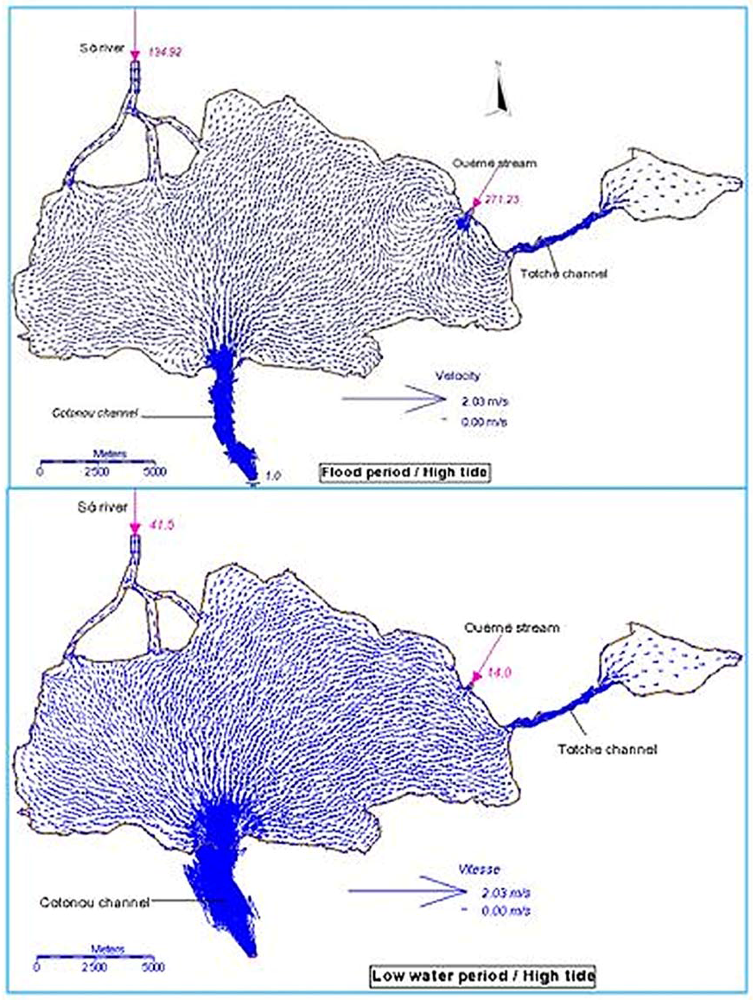
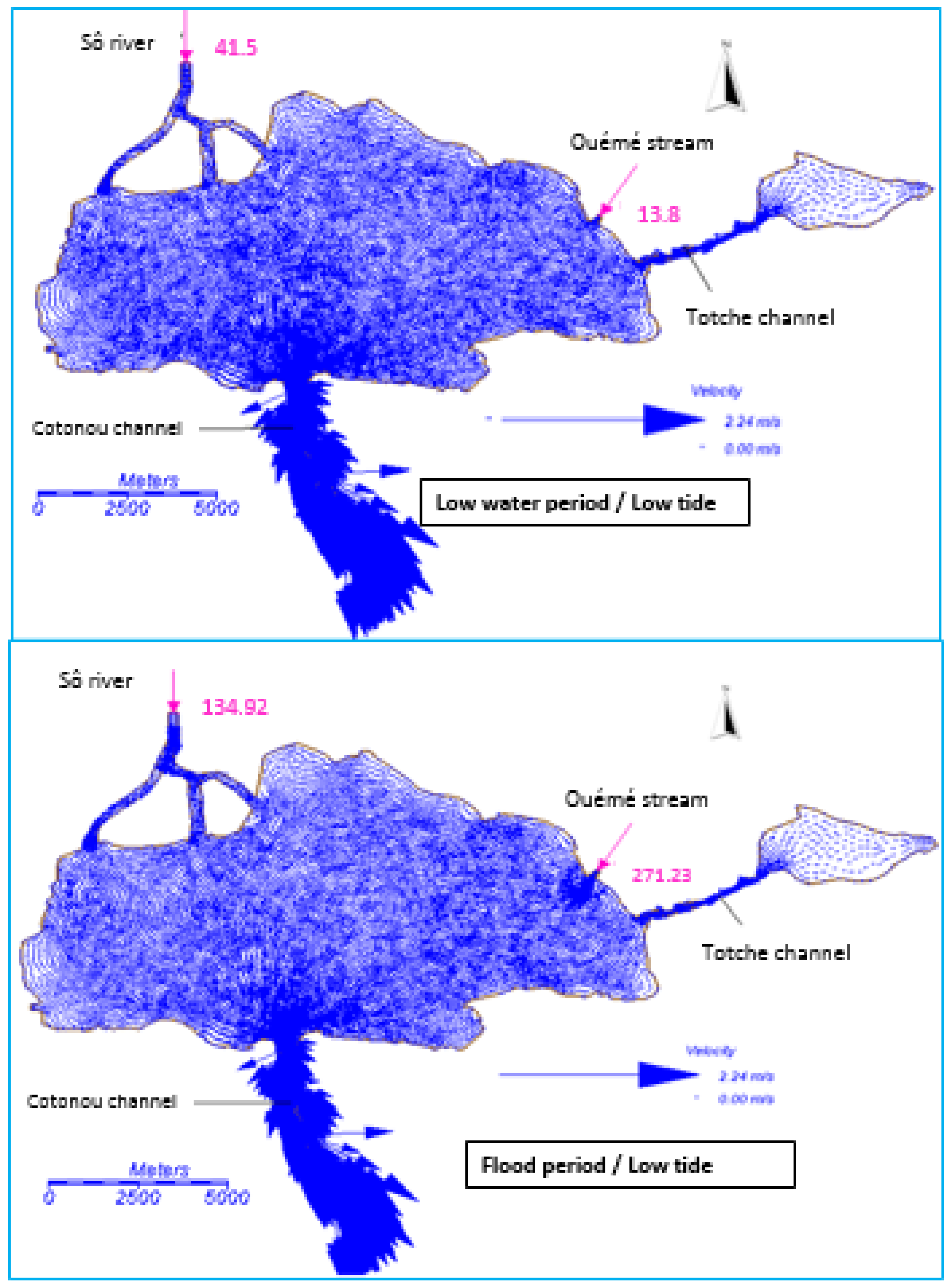
3.3.3. Velocity Field on the Lake Complex
Through the Cotonou channel, the lake filling takes place during the high tide and drains during low tide. In a flood period and average amplitude tide, the velocity field in the lake during filling (in high tide) indicates that the maximum speed (up to 0.6 m/s) is located at point 1, i.e., at the entrance of the channel in the sea. In a period of high amplitude tide, the velocities are about 1.21 and 1.37 m/s respectively during flood and low water period (Figure 10). Also in this filling period, all velocities are directed towards the lake. Once at the entry of the lake, the current repels water to the East Zone, the middle of lake, and Totche channel. On the other hand, during emptying, we note a velocity of 1.32 and 1.8 m/s during low water period respectively at average and high amplitude tide (Figure 11). The speeds calculated in the drain are all higher than those observed during the filling, favoring the renewal of the lake water. This is similar to results obtained by [26] in tagus estuary and contrary to those observed by [9] indicating a decrease of about 30% speed when leaving the high tide to low tide.
The rates decrease gradually away from point 1 to achieve values near-zero in the lake. Indeed, the maximum value observed in point 4 (in the lake) both during flood and low water period is 0.03 m/s, while the minimum is 2.5 × 10⁻⁴ m/s. When the tidal wave arrives at the lake, the speed of the waves depends on the depth. In the lake, the depth decreases, thus also the waves are refracted [27].
As the tidal wave propagates into shallower waters inside systems, it becomes distorted due to the effect of several physical processes, like bottom friction and momentum advection [28]. Besides the lateral convergence/divergence effect on tidal amplitude increase/decrease, the margin geometry, jointly with the bottom topography, were found by other authors, such as [29], as the principal constraint of the tidal currents direction.
At low tide, the opposite movement is observed, including aspiration of the lake to the Cotonou channel in which water bodies are moving towards the sea trip.
During a flood period, the entire upstream part of the estuary has a river traffic in the sense of an ebb. High flow rates under the average level of the lake do not allow the tide to reach most of the lake, which would justify the low salinity of the lake water in this period [17].
4. Conclusions
A two-dimensional hydrodynamic model (SMS) was successfully implemented for Nokoué lagoon. Results show that the calibration of the models was successfully carried out, revealing a good agreement between measurements and predictions. The validation tests showed that the models can reproduce an independently observed data set. However, the model does not accurately reflect the amplitude of variations. The defects observed seem minor and are not of a nature to jeopardize the ability of the model to reproduce the hydrodynamics of Nokoué Lake.
The analysis of the hydrodynamic functioning revealed that the dynamic of the lake is controlled by the tributaries flows in a flood period and tide during a low water period. It is characterized by the dephasing and the flattening of the amplitude tide, which increase as we move away from the channel. In a flood period, contrary to the low-water period, incoming flows are higher than outflows, reinforced by the amplitude of the tide. The volumes of water exchanged allowed us to determine average renewal times that are longer during low water periods, especially with a small amplitude tide. In contrast, the shortest renewal times are noted in flood periods with high amplitude tide.
In this context, we plan to take into account the entire lake complex composed of: Lake Nokoué, Porto Novo lagoon and Cotonou channel. Additional measures including water depths, flows exchanged with the sea as well as those discharged by rivers must be carried out. These different measures should be made over longer periods, allowing us to improve the quality of the model and to make long-term simulations, which is a tool for decision-making.
Acknowledgments
Thank to the International Foundation for Science (IFS) for supporting this work.
Author Contributions
Abel Afouda proposed topic and provide guidance to the study, Mahmoud Moussa, trained us to use the model and supervised the work, josué Zandagba made the simulations and drafted Article, Obada Ezechiel collected the data and contributed to the drafting. All authors have read and corrected the paper.
Conflicts of Interest
The author declares no conflict of interest.
References
- Casini, M.; Mocenni, C.; Paoletti, S.; Pranzo, M. Model-based decision support for integrated management and control of coastal lagoons. In Proceedings of the European Control Conference, Kos, Greece, 2–5 July 2007; p. 8.
- Arfi, R.; Dufour, P.; Mayer, D. Phytoplancton et pollution: Premières études en baie de Biétry (Côte d’Ivoire). Traitement mathématique des données. Oceanol. Acta 1981, 4, 319–329. [Google Scholar]
- Zabi, G.S. Les peuplements benthiques lagunaires liés à la pollution en zone urbaine d’Abidjan (Côte d’Ivoire). In Proceedings of the Actes du Symposium International sur les lagunes côtières, Scor/Labo/Unesco, Bordeaux, France, 8–14 September 1981; pp. 441–455.
- Guiral, D.; Lanusse, A. Contribution à l’étude hydro-dynamique de la baie de Biétri, lagune Ebrié, Côte d’Ivoire. Doc. Sci. Cent. Rech. Océano. Abidj. 1984, 15, 1–18. [Google Scholar]
- Arfi, R.; Guiral, D. Un écosystème estuarien eutrophe: La baie de Biétri. In Environnement et Ressources Aquatiques de Côte d’Ivoire. T.II. Les milieux lagunaires; Durand, J.R., Dufour, P., Guiral, D., Zabi, S., Eds.; ORSTOM: Paris, France, 1994; pp. 59–90. [Google Scholar]
- French Research Institute for Exploitation of the Sea (IFREMER). Réseau de Suivi Lagunaire du Languedoc-Roussillon; Bilan des Résultats 2002; IFREMER: Issy-les-Moulineaux, France, 2003; p. 36.
- Moussa, M. Modélisation Dynamique des Milieux Lacustres et Marins, et Dispersion de Polluants. Cours de Mécanique des Fluides Environnementale; ENIT: Tunisie, 2013; 136p. [Google Scholar]
- Derolez, V.; Fiandrino, A.; Munaron, N. Bilan Sur Les Principales Pressions Pesant Sur Les Lagunes Méditerranéennes et Leur Lien Avec l’état DCE; IFREMER: Issy-les-Moulineaux, France, 2014; p. 46. [Google Scholar]
- Capo, S. Hydrodynamique et Dynamique Sédimentaire en Milieu Tropical de Mangrove, Observations et Modélisation de L’estuaire du Konkouré, République de Guinée. Ph.D. Thesis, de l’Université de Bordeaux en Géologie Marine, Océanographie, France, 2006; p. 260. [Google Scholar]
- Rezgui, A.; Ben Maiz, N.; Moussa, M. Modélisation du fonctionnement hydrodynamique et écologique du Lac Nord de Tunis. Revue des Sciences de l’Eau 2008, 21, 349–361. [Google Scholar] [CrossRef]
- Monde, S.; Coulibaly, A.S.; Wognin, V.A.I.; Brenon, I.; Aka, K. Hydrological modelling of a two-outlet tropical lagoon (Ebrié lagoon, Ivory Coast) during an exceptional flood of the Comoé river. J. Environ. Hydrol. 2011, 19, 13. [Google Scholar]
- Wango, T.E.; Moussa, M.; N’Guessan, Y.A.; Monde, S. Hydrodynamique du complexe lagunaire Grand-Lahou, Ebrié et Aby (Côte d’Ivoire): Impacts des forçages fluviaux et de la marée. Bull. Inst. Sci. Rabat Sect. Sci. Terre 2013, 35, 27–38. [Google Scholar]
- Hilmi, K.; Makaoui, A.; Idrissi, M.; Abdellaoui, B.; El Ouehabi, Z. Circulation marine de la lagune de nador (maroc) par modelisation hydrodynamique. Eur. Sci. J. 2015, 11, 32. [Google Scholar]
- Albaret, J.J. Les peuplements des estuaires et des lagunes. In Les Poissons Des Eaux Continentales Africaines: Diversité, Écologie, Utilisation par L’homme; Lévêque, C., Paugy, D., Eds.; Éditions de l’IRD: Paris, France, 1999; pp. 325–349. [Google Scholar]
- Dehotin, U.A.; Laleye, P.A.; Dauta, A.; Moreau, J. Facteurs écologiques et diversité piscicole d’une lagune Ouest Africaine: Le lac Nokoué au Bénin. J. Afrotrop. Zool. 2007, 49–55. [Google Scholar]
- Surface Water Modelling System (SMS). Users Guide to RMA2; US Army Corps of Engineer-Waterways Experiment Station: Vicksburg, MS, USA, 2009; p. 296. [Google Scholar]
- Mama, D. Méthodologie et Résultats du Diagnostic de L’eutrophisation du lac Nokoué (Bénin); Ecole Doctorale Science Technologie et Santé, Université de Limoge: Limoge, France, 2010; p. 157. [Google Scholar]
- Cheng, R.T.; Burau, J.R.; Gartner, J.W. Interfacing data analysis and numerical modeling for tidal hydrodynamic phenomena. In Tidal Hydrodynamics; Parker, B.B., Ed.; Wiley: New York, NY, USA, 1991; pp. 201–219. [Google Scholar]
- Fernandes, E.H.L.; Dyer, K.R.; Niencheski, L.F.H. Calibration and validation of the TELEMAC-2D Model to the Patos Lagoon (Brazil). J. Coast. Res. 2001, 34, 470–488. [Google Scholar]
- Wango, T.D.; Moussa, M.; Adopo, K.L.; Mondé, S. Calage du modèle hydrodynamique à 2D du complexe lagunaire de Côte d’Ivoire. Geo-Eco-Trop 2011, 35, 23–32. [Google Scholar]
- Nash, J.E.; Sutcliffe, J.V. River flow forecasting through conceptual models. A discussion of principles. J. Hydrol. 1970, 10, 282–290. [Google Scholar] [CrossRef]
- Cheng, R.T.; Casulli, V.; Gartner, J.W. Tidal, residual, intertidal mudflat (TRIM) model and its applications to San Francisco Bay, California. Estuar. Coast. Shelf Sci. 1993, 36, 235–280. [Google Scholar] [CrossRef]
- Lawrence, G.A.; Ashley, K.I.; Yonemitsu, N.; Ellis, J.R. Natural dispersion in a small lake. Limnology and natural dispersion in a small lake. Limnol. Oceanogr. 1995, 40, 1519–1526. [Google Scholar] [CrossRef]
- List, E.J.; Gartrell, G.; Winant, C.D. Diffusion and dispersion in coastal waters. ASCE J. Hydraul. SCE J. Hydraul. Eng. 1990, 116, 1158–1179. [Google Scholar] [CrossRef]
- Hsu, M.H.; Kuo, A.Y.; Kuo, J.T.; Liu, W.C. Procedure to calibrate and verify numerical models of estuarine hydrodynamics. J. Hydraul. Eng. 1999, 125, 166–182. [Google Scholar] [CrossRef]
- Dias, J.M.; Valentim, J.M. Numerical modeling of Tagus estuary tidal dynamics. In Proceedings of the 11th International Coastal Symposium, Szczecin, Poland, 9–13 May 2011; pp. 1495–1499.
- Olympiades de physiques. Des ondes à la surface de l’eau:une histoire qui fait des vagues. Available online: http://odpf.org/images/archives_docs/18eme/memoires/gr-23/memoire.pdf (accessed on 1 May 2016).
- Pugh, D.T. Tides, Surges and Mean Sea-Level: A Handbook for Engineers and Scientists; John Wiley & Sons: Chichester, UK, 1987; p. 472. [Google Scholar]
- Neves, F.J. Dynamics and Hydrology of the Tagus Estuary: Results from In Situ Observations. Ph.D. Thesis, Universidade de Lisboa, Lisboa, Portugal, 2010; p. 210. [Google Scholar]
Figure 1.
Location map of Nokoué Lake (Benin).

Figure 2.
Bathymetric map and meshing of Nokoué Lake.

Figure 3.
Variation of the tide during calibration period.

Figure 4.
Variation of the water depth observed and simulated during calibration.

Figure 5.
Variation of the water depth observed and simulated in flood and low water period during validation.
Figure 5.
Variation of the water depth observed and simulated in flood and low water period during validation.

Figure 6.
Variation of the water surface elevation simulated with average (a) and high (b) tidal amplitude in flood period.
Figure 6.
Variation of the water surface elevation simulated with average (a) and high (b) tidal amplitude in flood period.

Figure 7.
Variation of the water surface elevation simulated with average (a); and high (b) tidal amplitude in low water period.
Figure 7.
Variation of the water surface elevation simulated with average (a); and high (b) tidal amplitude in low water period.

Figure 8.
Spatial and seasonal variation of the water surface elevation. (A) Low water period/Average Tidal amplitude/High tide; (B) Flood period/Average Tidal amplitude/High tide; (C) Low water period/High Tidal amplitude/High tide; (D) Flood period/High Tidal amplitude/High tide; (E) Low water period/High Tidal amplitude/low tide; (F) Flood period/High Tidal amplitude/low tide.

Figure 9.
Diurnal cycle of flow during low water period (a); and flood period (b).
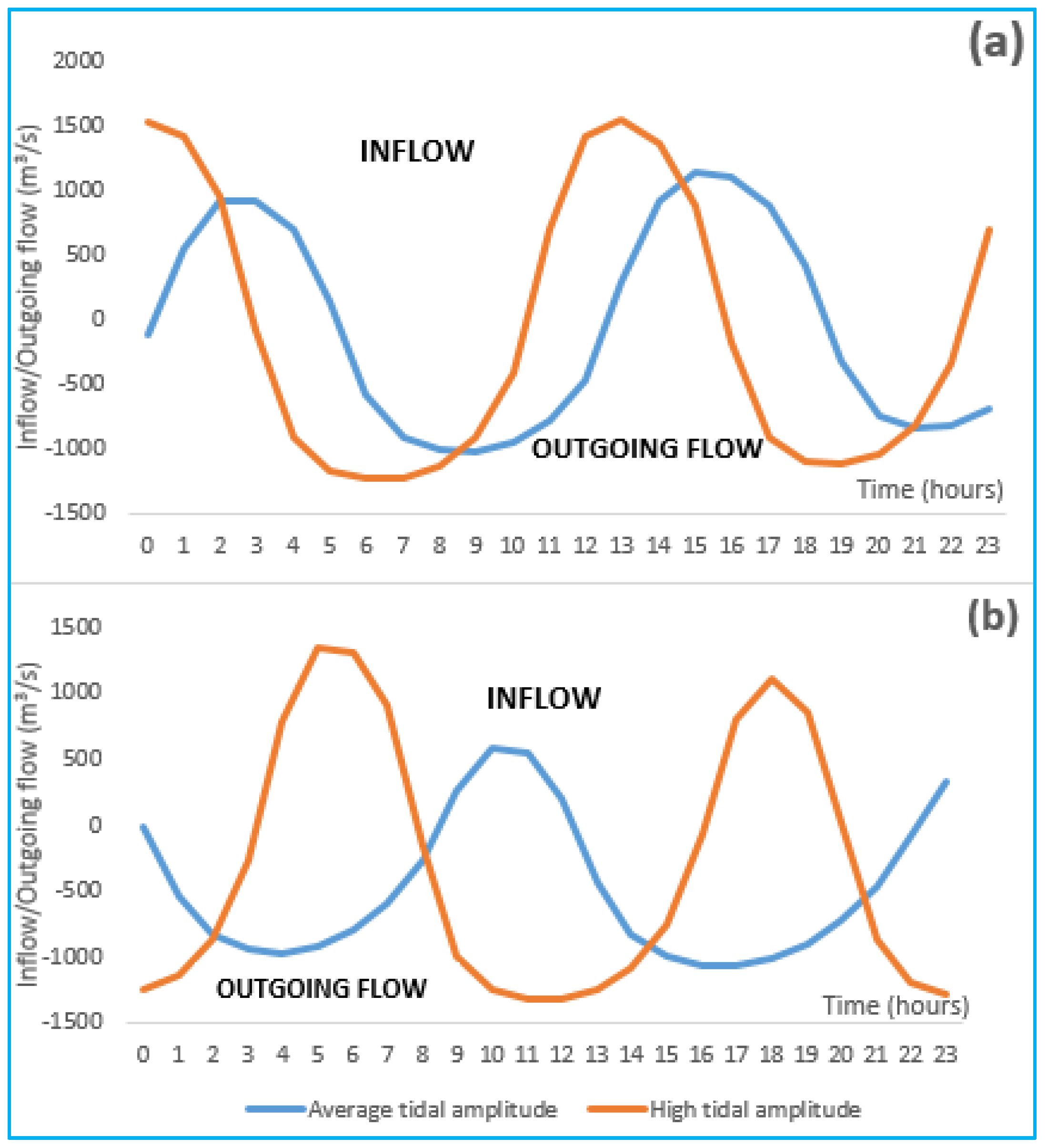
Figure 10.
Velocity field distribution during the filling of the lake in flood and low water period.
Figure 10.
Velocity field distribution during the filling of the lake in flood and low water period.

Figure 11.
Distribution of velocity field during the emptying of the lake in flood and low water period.
Figure 11.
Distribution of velocity field during the emptying of the lake in flood and low water period.


| Lake Entrance | Calibration Period | Validation Period | Simulation Period | |||
|---|---|---|---|---|---|---|
| 16 to 20 October 2007 | Flood period (16 to 20 October 2008) | Low water period (19 to 23 December 2008) | Flood period (15 September to 15 October 2014) | Low water period (1 to 31 January 2015) | ||
| Average flow estimated (m3/s) | Sô | 90.11 | 124.1 | 38.24 | 134.92 | 41.5 |
| Ouémé | 150.8 | 243.5 | 5 | 271.23 | 13.8 | |
| Period | Tidal Amplitude | Day |
|---|---|---|
| Flood Period | High tidal amplitude | 8 October 2014 |
| average tidal amplitude | 1 October 2014 | |
| Low water period | High tidal amplitude | 20 January 2015 |
| average tidal amplitude | 9 January 2015 |
© 2016 by the authors; licensee MDPI, Basel, Switzerland. This article is an open access article distributed under the terms and conditions of the Creative Commons Attribution (CC-BY) license (http://creativecommons.org/licenses/by/4.0/).
Share and Cite
MDPI and ACS Style
Zandagba, J.; Moussa, M.; Obada, E.; Afouda, A. Hydrodynamic Modeling of Nokoué Lake in Benin. Hydrology 2016, 3, 44. https://doi.org/10.3390/hydrology3040044
AMA Style
Zandagba J, Moussa M, Obada E, Afouda A. Hydrodynamic Modeling of Nokoué Lake in Benin. Hydrology. 2016; 3(4):44. https://doi.org/10.3390/hydrology3040044
Chicago/Turabian StyleZandagba, Josué, Mahmoud Moussa, Ezéchiel Obada, and Abel Afouda. 2016. "Hydrodynamic Modeling of Nokoué Lake in Benin" Hydrology 3, no. 4: 44. https://doi.org/10.3390/hydrology3040044
Note that from the first issue of 2016, this journal uses article numbers instead of page numbers. See further details here.