The Role of Auxiliary Stages in Gaussian Quantum Metrology


1
School of Mathematics and Physics, University of Portsmouth, Portsmouth PO1 3QL, UK
2
Dipartimento di Fisica and MECENAS, Università di Bari, I-70126 Bari, Italy
3
INFN, Sezione di Bari, I-70126 Bari, Italy
4
Institute of Cosmology and Gravitation, University of Portsmouth, Portsmouth PO1 3FX, UK
*
Author to whom correspondence should be addressed.
Photonics 2022, 9(5), 345; https://doi.org/10.3390/photonics9050345
Submission received: 30 March 2022
/
Revised: 5 May 2022
/
Accepted: 6 May 2022
/
Published: 14 May 2022
(This article belongs to the Special Issue Quantum Optics: Entanglement and Coherence in Photonic Systems)
Abstract
:The optimization of the passive and linear networks employed in quantum metrology, the field that studies and devises quantum estimation strategies to overcome the levels of precision achievable via classical means, appears to be an essential step in certain metrological protocols achieving the ultimate Heisenberg-scaling sensitivity. This optimization is generally performed by adding degrees of freedom by means of auxiliary stages, to optimize the probe before or after the interferometric evolution, and the choice of these stages ultimately determines the possibility to achieve a quantum enhancement. In this work we review the role of the auxiliary stages and of the extra degrees of freedom in estimation schemes, achieving the ultimate Heisenberg limit, which employ a squeezed-vacuum state and homodyne detection. We see that, after the optimization for the quantum enhancement has been performed, the extra degrees of freedom have a minor impact on the precision achieved by the setup, which remains essentially unaffected for networks with a larger number of channels. These degrees of freedom can thus be employed to manipulate how the information about the structure of the network is encoded into the probe, allowing us to perform quantum-enhanced estimations of linear and non-linear functions of independent parameters.
1. Introduction
In recent years, much attention has been put in the study of metrological schemes that exploit quantum resources, such as entanglement and squeezing, to enhance the sensitivity in the estimation of physical properties beyond the possibilities of classical strategies, with applications to imaging [1,2], thermometry [3,4], mapping of magnetic fields [5,6] and gravitational waves detection [7], among others. One of the most emblematic quantum enhancements sought in quantum metrology is the renown Heisenberg limit [8,9,10,11,12,13,14,15,16,17,18,19,20,21,22,23,24,25,26,27,28], which consists in achieving a scaling of the estimation error in the number N of probes (typically photons, or atoms) of order of , which surpasses the classical (or shot-noise) limit .
Gaussian metrology, which specializes in the study of estimation schemes employing Gaussian states of light and squeezing as metrological resource [29,30,31,32], represents a promising path towards a feasible quantum-enhancement in estimation strategies and the Heisenberg-scaling sensitivity [33,34,35,36,37,38,39,40,41]. It exploits the possibility to reduce the intrinsic noise of the electromagnetic field quadratures below the quantum fluctuations of the vacuum. Such a reduced noise, together with relatively easy-to-implement experimental procedures to produce these squeezed-noise states, and their increased robustness to decoherence compared to entangled states, make the Gaussian approach of great interest for short-term applications of quantum technologies. A particular case analysed by quantum metrology is the estimation of a single unknown parameter that appears within a given optical linear network multiple times, affecting for example different interferometric components [34,35,36,38,42,43,44,45,46,47,48] (see Figure 1). This is the case of unknown temperatures or magnitudes of the electromagnetic field, which modifies the physical properties of the optical parts composing the network within the regime of passive and linear evolution of the probe. The field investigating this type of schemes is generally referred to as distributed metrology, since the unknown parameter is effectively distributed among multiple components of the network.
On the other hand, estimation schemes based on Gaussian metrology usually incur in the challenge of adaptivity, i.e., the fact that the protocol depends on the value of the parameter that tries to estimate [44,49,50,51,52]. A typical approach to deal with adaptivity in Gaussian metrology consists in limiting the values that the unknown parameter can take, for example restricting the working range of the estimation scheme only to small values of the parameter, a condition that is common in a typical interferometric setup [43,46,48,53]. However, this solution unfortunately excludes certain experimental situations which require the ability to perform a quantum-enhanced estimation of the unknown parameter without imposing restrictions on its value.
Remarkably, it has been found in a recent work that is possible to achieve Heisenberg-scaling sensitivity in the estimation of a given unknown parameter distributed in an arbitrary M-channel network with a Gaussian scheme that only requires a classical knowledge of the parameter to optimize the network, i.e., the unknown parameter must be known with a prior precision that can be achieved with a classical estimation strategy [35]. To implement this scheme, a single auxiliary optical network is required in order to correctly refocus the probe, a squeezed-vacuum state, into the only output port observed through homodyne detection after the interferometric evolution, and a classical knowledge on the unknown parameter is required to engineer this auxiliary network. In other words, since in general an arbitrary M-channel linear network which encodes an unknown parameter does not refocus the probe into a single output port, some degrees of freedom must be introduced in the network by adding an auxiliary stage, which need to be optimized through a classical estimation strategy, which assures that the refocusing is correctly performed [35].
Within this scheme, provided that the optimization of the degrees of freedom has been performed, and the probe is correctly refocused in the only observed output port, it is always possible to add a second auxiliary network, which represents further extra degrees of freedom introduced in the optical network. One may wonder how the choice of this further auxiliary stage, and thus the presence of extra degrees of freedom, can influence the estimation scheme. Remarkably, in Ref. [36] it has been shown that the extra degrees of freedom introduced with a second auxiliary network do not have a major impact on the precision of the estimation of the unknown parameter. In particular, for networks with a large number of channels, it was shown that a random choice of the non-optimized auxiliary network leaves the precision of the estimation scheme essentially unaltered [36]. Therefore, this auxiliary stage and the extra degrees of freedom can be used to manipulate the way the information on the structure of the network is encoded in the probe.
In Ref. [37] it has been shown that it is possible to employ the previous scheme to achieve the Heisenberg-scaling sensitivity in the estimation of suitable functions of multiple parameters, and to exploit the degrees of freedom introduced by the non-optimized network to control the form of the function that can be estimated. Despite, in principle, complications may arise due to the presence of multiple parameters, representing multiple sources of uncertainty, which require a more complex mathematical formalism to describe a multi-parameter scenario, it is possible to employ the further degrees of freedom to manipulate the way the information on the structure of the network is encoded into the probe, and ultimately control the function of the parameters that is estimated at the Heisenberg-scaling sensitivity [37]. It is worth mentioning that, although the task of estimating functions of unknown parameters can be easily performed estimating separately each single parameter, and then evaluating the function in the data post-processing analysis, the ability to directly estimate a global property (e.g., spatial average of a field, field-gradients, or non-linear functions) allows one to avoid the waste of resources to obtain superfluous information on each single parameter, hence its relevance in applications, such as evaluation of averages of magnetic fields or temperatures.
This review is organized as follows. First, we briefly review the general scheme presented in Ref. [35] for the estimation of a single distributed parameter in Section 2. In Section 3 we discuss the effect of the presence of a second auxiliary network on the precision of the estimation, showing that the extra degrees of freedom introduced after the optimization of the refocusing has been performed do not essentially affect the precision of the estimation scheme [36]. Lastly, we will see in Section 4 how it is possible to exploit the exceeding degrees of freedom of the auxiliary stages which are not employed to optimize the network in a network with multiple parameters to change the function that can be estimated at the Heisenberg-scaling precision [37]. We conclude presenting two examples. The first is a 2-channel network which allows to estimate a function of three parameters (two optical phases and a beam-splitter reflectivity) parametrized by some quantities that can be chosen arbitrarily through the auxiliary stages. We will see that, according to the choice of the auxiliary networks, the function estimated can be linear or non-linear in the three parameters. The second is a scheme for the estimation of any linear combination of parameters with positive weights. In particular, we will show how it is possible to employ this scheme when the unknown parameter are not only phase-shifts, but also reflectivities of beam-splitters, or more in general phases acquired through complex local networks.
2. Distributed-Parameter Quantum-Enhanced Estimation
We will start introducing the Gaussian estimation scheme for M-channel networks which achieves the Heisenberg-scaling sensitivity recently proposed in Ref. [35]. Let us consider an arbitrary linear passive network which depends on a single parameter possibly distributed among several components of the network. The preparation of the input probe consists in the injection of a single-mode squeezed vacuum state in the first port of an auxiliary linear and passive network , which is used to scatter the photons injected among all the modes. The input state in our protocol is therefore given by
where is the squeezing operator associated with the first channel with squeezing parameter , and is the M-channel vacuum state. The average number N of photons injected in the network is thus . At the output of , a further auxiliary network is employed to refocus all the photons into a single mode, namely the first one, in order to capture all the information about the parameter in a single channel, at which homodyne detection is performed with a given local oscillator phase . For a linear passive unitary , it is possible to introduce the unitary matrix U whose elements represent the single-photon transition amplitudes from the i-th input port to the j-th output port, defined by the map
We now introduce the unitary matrix associated with the evolution through the whole network . Then, we can write the probability
that a photon injected in the first port of comes out from the first port of , and the phase
accumulated through this interferometric evolution. One can show, by employing Cramér-Rao analysis [54,55], that it is possible to achieve Heisenberg-scaling sensitivity in the estimation of if the conditions
are satisfied, where and are arbitrary but both independent of N, and where is an optimal choice for the local oscillator phase. Under conditions (5), the ultimate precision achievable by this scheme with any estimator after iterations of the measurement is given by
where is the Fisher information associated with this estimation scheme, and
is an N-independent factor which reaches its maximum at and .
One can show that it is possible to optimize the refocusing network with only classical prior information on the parameter , namely after a classical strategy is employed to perform a prior coarse estimation of the unknown parameter.
In the following we will focus on the relation between the non-optimized auxiliary network , which yields further degrees of freedom in the linear network of the scheme, and the precision shown in Equation (6). Then, we will show how it is possible to employ these extra degrees of freedom to manipulate the function of multiple parameters that can be estimated with this scheme.
3. Typicality of Quantum Enhanced Sensitivity
In the previous section we have presented a generic protocol that allows us to achieve the Heisenberg limit in the estimation of a parameter distributed in an arbitrary network when conditions (5) are met. In particular, in order to satisfy condition (5b), either the scattering stage or the refocusing stage needs to be optimized after a classical prior estimation of the parameter is carried out. The remaining auxiliary stage is thus left completely arbitrary, and one may wonder how the choice of this stage can influence the precision of the estimation, and in particular the pre-factor appearing in the sensitivity in Equation (6). More precisely, it may happen that a particularly unfortunate choice of the non-optimized stage causes this pre-factor to vanish, for example if this auxiliary stage transforms the optical mode of the probe into a mode which is insensible on or independent of the value of the parameter (A trivial example is the case where the unitary matrix describing the network is , and the auxiliary stage is the identity , for . In this case the probe is left in the first channel of the network, which does not depend on .) In this section we will see that, for an arbitrary choice of the non-optimized auxiliary stage, the pre-factor tends to be far from zero, meaning that small values are mostly unlikely, especially for networks with a large number M of channels [36]. For simplicity, we will explicitly consider the case in which the refocusing stage has been optimized to satisfy condition (5b) while is left arbitrary, but similar considerations can be done in the opposite scenario due to the symmetry of the problem.
3.1. The Role of the Generator
We can link the pre-factor , appearing in Equation (6), to the derivative of the matrix element
When condition (5b) holds, Equation (8) simplifies to
so that the two quantities are equal up to a term of order . Condition (5b) can be recast in terms of a constraint on the form of
If we now introduce the (generally -dependent) generator
of the unitary matrix , we can further manipulate the pre-factor . Employing the definition of in Equation (11), and the relation in Equation (10), we can write
Equations (9) and (12) conveniently express the pre-factor as a function of the generator of the network and a unitary matrix independent of the optimized stage , so that ultimately we can write for large N
and thus the Fisher information appearing in the sensitivity in Equation (6) becomes
It is easy to see that the pre-factor can be written as the square of a convex combination of the eigenvalues of the generator . In fact, if we call the matrix whose columns are the eigenvectors of , so that , we can recast the pre-factor in terms of the eigenvalues
where , with by the unitarity of . If we suppose, without lack of generality, that the eigenvalues are ordered so that , the maximum value of the pre-factor is achieved for
namely when the first column of U coincides (up to a complex phase) with the first eigenvector of , belonging to the eigenvalue with the larger absolute value. Recalling that U represents the action of the input auxiliary stage (see Equation (12)), and that the elements of its first column coincides with the transition amplitudes from the first input channel (see Equation (2)), we can understand the meaning of the condition (16): the input stage must be chosen in order to maximize the effect of the network on the probe, which must evolve under the optical mode (not necessarily coinciding with a physical channel) which is most sensitive to the variations of —i.e., corresponding to the eigenvalue of with maximum absolute value. For a choice of U satisfying condition (16) (e.g., for ), the pre-factor in Equation (13) coincides with the highest eigenvalue of the generator squared
namely the squared norm of the generator . This coincides with the pre-factor of the maximum Quantum Fisher information for Gaussian states found in Ref. [44], meaning that the scheme presented in Section 2 is the optimal Gaussian strategy when also the auxiliary stage is optimized according to Equation (16).
3.2. Typical Behaviour of the Pre-Factor in the Heisenberg Scaling
Although the condition for the optimal choice of the unitary U has been easily found, the eigenvectors of in general depend on the value of the distributed parameter , and on the structure of the network , and so do the solutions of Equation (16). On the other hand, one may be interested in the case in which no prior knowledge on the structure of —and thus on —is given. In general, with these assumptions, finding the optimal stage that maximizes the pre-factor and satisfies condition (16) is impossible. Instead, in this scenario, it becomes more appropriate to study the behaviour of the pre-factor for arbitrary choices of the auxiliary network, and ultimately of the non-fixed degrees of freedoms introduced with it. In particular, one may be interested in knowing how likely the value of is equal or close to zero, when the auxiliary stage is chosen at random. However, to introduce concepts such as ‘how likely’ and ‘at random’, we must somehow endow the set of all the auxiliary linear network with a probability measure. Conveniently, there is already a mathematical structure which well represents this set, which we have already extensively employed: every M-channel linear and passive network is described through the action of a unitary matrix, and the ‘composition rules’ of linear networks is well represented by the composition rules of U(M), the group of unitary matrices.
Since we are supposing that we do not possess any prior information on the structure of , all the auxiliary stages U are equivalent candidate to achieve the optimal value for the pre-factor. For this reason, we can endow U(M) with its Haar measure [56]. This is the measure on the space of the unitary matrices that generalizes the uniform distribution on finite intervals of . In fact, the Haar measure on U(M) is defined so that the measure of any open subset is invariant under left or right unitary transformations, namely , for every . In other words, it is a measure that only depends on the ‘size’ of the subsets of U(M). Once we have chosen the prescription to sample the network U, we are able to evaluate statistical properties of the pre-factor . In particular, we show in Appendix A that
is the expectation value of the pre-factor (13) over random choices of the matrix U, with respect to the Haar measure. In the case of a generator proportional to the identity , which corresponds to a network made of M identical copies of single-channel unitaries acting in parallel (This condition is satisfied for example for the metrological scheme introduced in Ref. [12], although in such a case the generator is independent of ), we have and , so that the average value of the pre-factor equals the maximum in Equation (17). Indeed, with this kind of network, the auxiliary stage which distribute the probe on all M channels becomes irrelevant, since the network acts identically in each channel. Indeed, in such a case any unitary matrix diagonalizes the generator and therefore Equation (16) is satisfied for any .
In general, an average value of the pre-factor close to the maximum in Equation (17) is favourable to a smaller value, since it implies a better Fisher information and a better precision in average. The only case for which is equal to zero is when the whole generator is vanishing, occurrence happening only for networks which do not actually depend on the unknown parameter. A generator with small eigenvalues—i.e., a network which is not very sensitive to the variations of the parameter —would cause the average in Equation (18) to decrease, diminishing the average precision of the estimation scheme. However, it is possible to find a lower bound on the average value (18) using Jensen’s inequality to obtain
(see Appendix A). We notice how the right-hand side term in Equation (19) is the squared average of the eigenvalues of . This means that if we are able to control the value of the average of the generator, say in such a way that it is larger of a certain fraction of the norm of the generator, i.e., , then it follows from Equation (19) that we can assure that the average of the pre-factor is larger than a fraction of its maximum value .
Even though we may be able to control the average of through Equation (19), it may happen that the typical values that the pre-factor takes are far from , for random choices of the unitary U. A paradigmatic example of a random variable which typically takes very different values than its average is a quantity which can only be equal to 0 or 1 with equal probabilities: in such case, its average is never an effective outcome of the random variable, let alone typical. Fortunately, this is not the case for the pre-factor , which is instead a well-behaved function of the random unitary U. In fact, we see in Appendix A that is instead typical for networks with many channels, i.e., that it is possible to apply results on the concentration of measure in high-dimensional spaces, which assure that becomes almost constant for random choices of for large M, and thus it concentrates around its average value
with . This results tell us that, for an arbitrary choice of auxiliary stage , the value of the pre-factor appearing in the Fisher information in Equation (14) is with overwhelming probability close to its average, for networks with a large enough number of channels M (see Figure 2). Moreover, Equation (19) shows that it is possible to bound from below the average of the pre-factor, if some control on the average of the eigenvalues of is possible. This shows that, beside very unlikely exceptions, the choice of the non-optimized stage is mostly irrelevant as for the precision of the estimation scheme. In the next section, we will see how it is possible to exploit the additional degrees of freedom introduced by the non-optimized network to manipulate how the information on the structure of the network is encoded in the probe. This will give us some freedom in choosing the function of a given set of parameters that can be estimated with the Heisenberg limit precision.
4. Estimation of Functions of Parameters
In the previous section, we have seen that it is always possible to add a -independent auxiliary stage to the estimation setup shown in Section 2, which introduces degrees of freedom that essentially do not affect the precision of the estimation scheme, especially for networks with a large number of channels. A natural question that may arise is whether the same setup can be employed in achieving the Heisenberg limit when the number of unknown parameters affecting the arbitrary network increases, and if it is possible to employ these degrees of freedom to select a specific function of the parameters that can be measured with Heisenberg-scaling sensitivity. Although such task can be performed estimating separately each single parameter, and then evaluating the function during the data analysis, the ability to directly estimate a global property (e.g., spatial average of a field, field-gradients, or non-linear functions) allows us to not waste resources to obtain superfluous information on each single parameter. However, it cannot be excluded in principle that complications may arise due to the presence of multiple sources of uncertainty, complications which already materialize starting from the more complex mathematical formalism required to describe the multi-parameter scenario [57,58].
In this section we will describe a scheme for the estimation of functions of multiple parameters encoded in a generic linear passive network [37]. We will show that, employing a single squeezed vacuum state and a single homodyne detector, i.e., the same probe and measurement of the setup shown in Section 2, it is possible to reach the Heisenberg limit in the estimation of functions of the parameters, satisfying conditions that are similar to the ones found for the single-parameter scheme. We find also in this scenario that a classical knowledge on the unknown parameters is required to optimize the network through the use of auxiliary stages, allowing us to conceive two-steps protocols achieving the Heisenberg limit. Moreover, we will see how the exceeding degrees of freedom of the auxiliary stages which are not employed to optimize the network can be used to change the functional dependence between the quantity that can be estimated and the unknown parameters.
Once we will have described the estimation scheme and discussed the conditions that need to be met in order to reach the Heisenberg limit, we will present two examples. The first is a 2-channel network which allows us to estimate a function of three parameters, of which two optical phases and a beam-splitter reflectivity, parametrized by some quantities that can be chosen arbitrarily through the auxiliary stages employed. We will see that, according to the choice of the auxiliary networks, the function estimated can be linear or non-linear in the three parameters. The second is a scheme for the estimation of any linear combination of parameters with positive weights. In particular, we will show how it is possible to employ this scheme when the unknown parameter are not only phase-shifts, but also reflectivities of beam-splitters, or more in general phases acquired through complex local networks.
4.1. Setup
Let us consider a M-channel linear and passive network which depends on p unknown parameters . The parameters may represent certain physical properties associated with each component of the network, such as reflectivities of beam-splitters, or phase-shift magnitudes, or they may be the values of external non-uniform fields which influence several components of the network, such as the temperature and the electromagnetic field (see Figure 3). The action of the network can be described with the usual unitary matrix representation , defined through Equation (2). The probe employed is the same as shown in Equation (1), injected in a single input port of an auxiliary network , say the first, with number of photons in average in the probe. In order to infer some information on the parameters from the interferometric evolution of the probe, we will perform homodyne measurements at a single output port, say the first, of the quadrature , where is the phase of the local oscillator. Similarly to the setup described in Section 2, we will consider in this model the presence of a further refocusing network acting on the probe after the evolution given by the network respectively. Intuitively, the role of the stage is to distribute the probe among all the channels of the network, while refocuses the probe into the only output port which is observed. However, in light of the results of typicality presented in Section 3, which showed that the overall precision of the single-parameter estimation scheme is essentially not affected by the choice of the non-optimized network for a large number M of channels, we will exploit the remaining degrees of freedom in the two auxiliary stages to manipulate how the information about the structure of the network and on the parameters is encoded into the probe.
Since the photons of the probe are all injected in the first channel, and only the first output port is observed, the only relevant element of the unitary matrix —representing the action of the whole setup on the probe—is , namely the transition amplitude from the first input to the first output port. We will employ the parametrization
which emphasizes the two relevant physical quantities, i.e., the transition probability and the phase acquired by the probe through the network, which is in general a function of the unknown parameters . We will see later that the function can be estimated at the Heisenberg limit. After the interferometric evolution, the squeezed variance hence becomes . If the quadrature is observed through homodyne detection, the probability distribution which governs the outcomes of the measurement is Gaussian, due to the Gaussian nature of the probe [30], and centred in zero, due to the absence of displacement. We thus write the Gaussian probability distribution
with variance calculated in Appendix B
and can be thought as the average between the noises of the vacuum and of the squeezed states, weighted by the factors and respectively.
The presence of multiple independent parameters imposes the multi-parameter approach for the analysis of the ultimate precisions achievable with this setup, and the use of the Fisher information matrix [54,55],
By plugging Equation (22) into Equation (24) one gets
where . Having the probability distribution in Equation (22) a null displacement, all the information on the parameters is encoded in the variance through the transition probability and the phase acquired . It is thus convenient to separate the derivative of the variance in Equation (23) in two contributions
where and denote the partial derivatives with respect to P and f, so that we easily obtain from Equation (23)
4.2. Heisenberg Scaling
We can see from Equations (23)–(27) that, if no specific conditions are imposed on the network , the Fisher information matrix cannot generally reach the Heisenberg limit. This is due to the presence of the squared variance at the denominator of Equation (25), which may grow with order , with N number of photons injected, since
while the derivatives in Equation (27) only contain terms of the type and , which are of order N. Thus it arises the need to impose conditions which prevent the variance of the observed quadrature to grow with the number of photons. We show in Appendix C that this setup reaches the Heisenberg limit in the estimation of if similar conditions to the ones in Equation (5) for the single-parameter scenario are met. In particular, the conditions are
with k and ℓ arbitrary factors which are independent of N. In Section 4.3, we will discuss about the meaning of the conditions in Equation (29), exploring their consequences and highlighting the similarities with the single-parameter protocol in Section 2. In Appendix C we show that, when conditions (29) are met, the Fisher information matrix in Equation (25) becomes
where is the same N-independent constant factor defined in Equation (7) for the single-parameter estimation.
Despite the presence of the factor in the Fisher information matrix in Equation (30), it is generally impossible to reach the Heisenberg limit in the estimation of each of the p parameters . In fact, we can easily see that the (asymptotic) expression of the Fisher information matrix (30) is non-invertible: the (column) vector is trivially the only eigenvector associated with a non-vanishing eigenvalue of the Fisher information matrix. As discussed in Refs. [59,60], a singular Fisher information matrix is symptomatic of the presence of parameters which do not admit estimators with finite variances, and the traditional multi-parameter Cramér-Rao bound [54,55]
is not applicable due to the non-invertibility of . In fact, only specific functions of the parameters admit unbiased estimators with finite variance [59,60]. In particular, specialized to the Fisher information matrix of the problem at hand in Equation (30), the functions which admit finite variance are the ones satisfying [59]
The solutions of Equation (32) for all the possible values of are of the form , with independent of , and in particular belongs to this family, which entails the fact that the function can be estimated with finite variance. We can finally evaluate the Cramér-Rao bound associated with any estimator of , obtaining in the asymptotic regime (see Appendix E)
which reaches the Heisenberg limit in the mean number of photons N.
Lastly, it is worth to mention that we can saturate the Cramér-Rao bound in the limit of large samples, namely it is always possible to find an estimator, the maximum-likelihood estimator , which is unbiased and efficient in the asymptotic regime of large samples [55]. In order to find the maximum-likelihood estimator, we need to maximize the Likelihood function
In Appendix D we see that the solution which maximizes the Likelihood function (34) is given by the estimator satisfying
where is the variance in Equation (23) as a function of , supposing that satisfies Equation (29b) and is known, while is the usual sample variance
Inverting the function , we can obtain the explicit expression of the maximum-likelihood estimator in this regime
with n integer. We notice that the presence of the cosine function, which is invertible only on intervals of its argument of the type , requests a prior knowledge on the argument in order to choose the correct value of n in Equation (37). However, we will discuss in the next section that a classical coarse estimation of the parameters is required in order to optimize the network and satisfy condition (29b). In other words, the error committed in the prior coarse estimation must be of order , decreasing at the SQL with the number of photons N. For a large enough N, will be small enough to unequivocally choose the correct interval of invertibility of the cosine, and thus the correct n in Equation (37).
4.3. On the Conditions for the Heisenberg Scaling
Despite the presence of multiple parameters, the substantial similarity of conditions (29) with the single-parameter counterparts in Equation (5) allows us to draw the same consideration discussed for the single-parameter scheme in Ref. [35]. Condition (29a) is a minimum resolution requirement on the tuning of local-oscillator phase , which must be controlled with steps of order . Moreover, the requirement in Equation (29a) implies that must be tuned in such a way to measure a quadrature field which is slightly different from the minimum-variance quadrature . This can be explained by the fact that the minimum variance—i.e., for —is a stationary point for variations of , and hence its gradient in Equation (26) is vanishing for close to its maximum and to its minimum.
Condition (29b) is a requirement on the refocusing of the probe into the only observed channel. In order for the variance in Equation (23) of the observed quadrature to be ‘squeezed’—i.e., —the contribution of the vacuum must be of order . Moreover, similar considerations also for the prior knowledge on the parameter required for the optimization of the refocusing network can be drawn. First of all, condition (29b) can be satisfied by only optimizing a single auxiliary stage, while choosing arbitrarily the other. We can call the result of a prior coarse estimation of the parameters required to optimize a single auxiliary stage, say . The single-photon probability transition can be written as the squared modulus of the scalar product of the two vectors and , with
where is a smooth function of and which is maximized for , since would satisfy . For small deviations of the coarse estimation from the true values of the parameters , we can expand Equation (38)
where the gradient is zero for . Thus, also in the presence of multiple unknown parameter , if the errors in the prior estimations are of order , it becomes possible to engineer the refocusing stage that satisfies condition (29b), and thus that allows to reach the Heisenberg limit, similarly to the single-parameter estimation protocol.
4.4. Examples of Quantum-Enhanced Estimation of Functions
The presence of two auxiliary stages and , and the need to optimize only one of them in order to satisfy condition (29b)—and ultimately to reach the Heisenberg limit—entail the possibility to exploit the remaining degrees of freedom in the network to manipulate how the information on the parameters are encoded in the probe. In this section, two examples are proposed, which make use of these degrees of freedom to allow us to choose the function to be estimated from a family of functions of some parameters . The first example is a 2-channel network for the estimation at the Heisenberg limit of non-linear functions of three parameters, of which two are magnitudes of phase-shifts and one is the reflectivity of a beam-splitter. The second is a network for the estimation of linear combination with positive weights of an arbitrary number of parameters.
4.4.1. Non-Linear Functions
We here consider a 2-channel network for the estimation of non-linear functions of the reflectivity of a beam-splitter and the magnitudes of two phase-shifts , with reference to Figure 4. The functions are parametrized by the quantities , which can be implemented arbitrarily, with the only condition that . The possibility to choose the quantities stems from the presence of abundant degrees of freedom in the auxiliary networks and , which are not employed for the optimization of the network needed to satisfy Equation (29b). The protocol employed is the same considered in Section 4.1, with a single squeezed-vacuum state with average number of photons injected in the first input port of the overall network, with r squeezing parameter of the probe, and only the first output channel observed through homodyne detection, to measure the quadrature , where is the phase of the homodyne local oscillator.
We can write the matrices representing the action of the beam-splitter and the phase-shifts in the network as
respectively, where , , is the i-th Pauli matrix and is the identity matrix, so that the network is represented by the matrix
The quantity that we will use to parametrize the family of functions is the relative phase between the arms of the input auxiliary stage , which is overall described by the unitary matrix
This auxiliary network consists of two phase-shifts of arbitrary magnitudes and in the first and second channel, and a beam splitter with reflectivity
which can be engineered once a classical estimation of the unknown reflectivity of the beam-splitter in has been carried out, namely after a coarse prior estimation so that the error is of order . The refocusing auxiliary network is described, with reference to Figure 4, by the unitary matrix
where the quantity enters in the relative phase of the two channels, this time changed in sign. We can see from the expression of that this auxiliary stage in general depends on the classical estimation of the unknown parameters, namely on the results of a coarse prior estimation for which the committed errors are of order .
We will now see that the Heisenberg limit can be achieved in the estimation of the complex phase of the network depicted in Figure 4, showing that it satisfies condition (29b). In fact, employing Equations (41)–(44), we can explicitly evaluate the transition amplitude
where the quantity is defined in Equation (43). In Appendix F we see that the transition probability actually satisfies the condition (29b) on the network for the Heisenberg limit, which means that the auxiliary networks correctly operate on the probe so that it gets refocused on the only observed channel. In Appendix F the complex phase is evaluated
with
which is in general a non-linear function of the parameters . We see from Equations (46) and (47) how the choice of the arbitrary values of the parameters affects the functional dependence of the phase on the parameters , and thus of the quantity which can be estimated at the Heisenberg limit. In particular, beside the term which simply adds an overall phase, the relative phase affects the functional dependence between the quantity in Equation (47) and .
For example, for the beam-splitters in the auxiliary stages and become balanced—i.e., from Equation (43)—while the function of in Equation (46) we can estimate reduces to
thus becoming a linear function of the parameters. From Equation (45), we can evaluate the transition probability for the choice of , and for
which satisfies condition (29b) as expected, since the error in the coarse estimation are assumed to be classical, i.e., so that . Comparing Equations (29b) and (49), and assuming that with independent of N, it is easy to evaluate the factor
which enters through in Equation (7) in the Cramér-Rao bound in Equation (33). Moreover we notice that, if the two phase-shifts are completely known quantities, so that we are able to perfectly balance them with the auxiliary stage with , the overall network in Figure 4 reduces (up to a global phase ) to a setup which transform the reflectivity in an optical delay, without any prior information on the parameter. In fact in this case, the overall phase in Equation (48) becomes . In Section 4.4.2 we will make use of this type of networks specifically for this purpose, and be able to treat the reflectivities of beam-splitter as if they were simple phase-shift.
For , the reflectivity in Equation (43) becomes , while the function estimated at the Heisenberg limit in Equation (48) reads
where the term can be neglected since it is of order or smaller, i.e., beyond the Heisenberg limit resolution. In particular, we notice from Equation (51) that is a relatively simple non-linear function, in which we can find the products and , between each phase-shifts and the transmittivity amplitude of the beam-splitter. If we once again evaluate the transition probability from Equation (45) for we obtain
which satisfies condition (29b) as expected, since is of order . In particular, we can easily evaluate the N-independent factor
which enters in the Cramér-Rao bound in Equation (33), if we assume with independent of N. If moreover , the network in Figure 4 reduces to a balanced Mach-Zehnder, which allows us to estimate the average of the two phase-shifts since the overall phase in Equation (51) reduces, for , to
where the average of the two phase-shifts and sums a known quantity, which can thus be subtracted during the estimation without affecting the overall precision. In the next example, we will generalize such scheme, considering a similar network, but with an arbitrary number of channels and generally unbalanced beam-splitters.
4.4.2. Linear Combinations of Arbitrary Parameters
We now consider a network which depends on M independent parameters (see Figure 5), that allows us to estimate with a precision at the Heisenberg limit any linear combination
with positive weights . As also discussed previously in this chapter, the ability to change arbitrarily the weights stems from the presence of degrees of freedom in the auxiliary stages and that are not employed to refocus the probe in the only observed channel, i.e., to satisfy condition (29b). At first, we will suppose that the parameters can either be magnitudes of phase-shifts or reflectivities of beam-splitters. Later, we will show how it is possible to generalize the scheme for an arbitrary set of parameters. We will also suppose, without loss of generality, that the weights sum to one, namely that the linear combination in Equation (55) is a convex sum. To estimate a generic linear combination, it would suffice to rescale the estimated convex sum, causing a rescaling of the error in the estimation which does not affect the Heisenberg limit.
With reference to Figure 5, we now describe the network affected by M unknown parameters . The parameters act in parallel, in the sense that the i-th parameter only affects the i-th mode of the network, and they can equivalently be the magnitudes of a phase-shift or the reflectivities of beam-splitters , with the second Pauli matrix. For each unknown beam-splitter, a 2-channel passive and linear network is employed in , whose purpose is to transform the reflectivity into a relative phase between the two ports of the beam-splitter (see the panel (b) in Figure 5). This can be done through the network
with
We also remark that, despite each mode of with an unknown beam-splitter is practically composed of two separated channels, the overall network in Equation (56) acts as a phase-shift in each of the two channels, namely the two modes are not mixed. Since this local network is only fed through a single input port, it essentially acts as a single-channel phase shift of magnitude on the probe, depending on which of the two arms are employed. The overall network can be thus described with the unitary matrix
regardless of the nature of the parameters , whether they are phase magnitudes or beam-splitter reflectivities.
The input auxiliary stage is a M-channel generalized beam-splitter, which scatters the probe injected in the first input port into each of the M channels of according to the weights . Specifically, the unitary matrix representing the input network is chosen so that
Noticeably, this constraint is -independent, i.e., does not need to be optimized after a prior coarse estimation of . The output auxiliary network can be though as been composed of three separate stages. First, a phase shift of magnitude is applied to the i-th channel, where is a coarse estimate of the prior classical measurement of , so that the error committed is of order . Then, a second generalized beam-splitter which does not depend on is in place, whose purpose is to invert the action of and thus refocusing the probe into the first channel of the network. Finally, a phase-shift of magnitude is applied before the homodyne detection at the first output port. The overall action of the network is thus described by the unitary matrix
where we denoted with .
With this setup, the probability amplitude found in Equation (21) can be easily evaluated through Equations (58)–(60), and it reads
where we can neglect the term , since it is of order and thus beyond the Heisenberg limit resolution we can achieve. We can now evaluate the transition probability through Equation (61)
which clearly satisfies condition (29b), so that the Heisenberg limit can be achieved in the estimation of the complex phase . We can thus evaluate, comparing Equations (29b) and (62), the factor ℓ which enters in the Fisher information shown in Equation (33),
where we supposed that with independent of N. From Equation (61) we obtain
so that it is possible to recover the linear combination (55) at the Heisenberg limit from the estimation of . We notice in fact that in (55) and the complex phase in (64) are equal up to a quantity of order , which is beyond the Heisenberg resolution, since the errors in the classical prior estimation are of order .
In conclusion, we will discuss about two different features of this protocol. First, we notice from Equation (56) that the network employed to transform the reflectivity of the beam-splitters into phase-shifts inverts the sign of the parameter in the second channel. This means that, if the portion of the probe which has been scattered into this network is injected in its second port, it acquires a phase . It is then possible to exploit this behaviour to estimate a linear combination which admits negative weights for the reflectivities of the beam-splitters, employing the same protocol described in this section with the only precaution to invert the sign of the classical estimation of this parameter. Second, it is possible to further generalize the local networks in each mode of . In fact, we can replace the networks in the panel of Figure 5 with a generic m-channel network and, provided that the probe comes out of this local network from a single output channel—i.e., the network acts as a phase-shift on the probe—the same results found in this section still apply. Not only, in Appendix G we show that it is not necessary that all the photons come out from a single output port of each local network: instead, it suffices that a similar refocusing condition to the one in Equation (29b) is satisfied locally by each . It is thus possible to conceive, for example, a scheme that allows to reach the Heisenberg limit in the estimation of linear combination of parameters and functions of parameters, if we choose as the whole network described in the example in Section 4.4.1.
5. Conclusions
The quantum metrological revolution is, at this moment in time, exciting and thrilling. The recent advances in the field of quantum mechanics have been incessantly stimulating the development of increasingly ingenious and innovative technologies which exploit the laws and rules of the microscopic world. Ranging from computing to biology, medicine, cosmology, imaging, sensing, cryptography and neural networks, quantum technologies appear to consistently outperform their classical counterparts. In particular, the fields of quantum sensing and quantum metrology propose schemes for the estimation of physical properties, such as lengths, time intervals, temperatures, and more, achieving enhanced levels of precision. In particular, the field of distributed Gaussian metrology, which studies strategies employing Gaussian states for the estimation of unknown parameters distributed arbitrarily on a passive and linear network, has recently witnessed some improvements in overcoming the challenge of adaptivity of the network, usually found in Gaussian and, more in general, quantum-enhanced schemes. In fact, as we briefly summarize in Section 2, employing a single squeezed vacuum state and performing homodyne detection at a single output port, it has been shown that it is possible to achieve the elusive Heisenberg-scaling sensitivity by only adding a single auxiliary network, whose purpose is to refocus the probe into the only observed channel. This auxiliary network, which introduced degrees of freedom in the interferometer, can be engineered with only a classical prior knowledge on the parameter.
The main focus of this review was then put on discussing the role and the effect of further degrees of freedom that can be added in the network, for example employing a second, non-optimized auxiliary stage. We have shown in Section 3 that this auxiliary stage leaves essentially unchanged the precision achieved by the setup, especially for networks with a large number of channel, and we have discussed how this result allows us to assume that the constant factor multiplying the Heisenberg scaling of the precision can be controlled and is typically far from zero. In Section 4 we demonstrated that it is possible to exploit this ability to manipulate how the information on multiple parameters encoded in a passive and linear network. We have seen that this results in the possibility to estimate functions of the unknown parameters which we can manipulate by acting on these further degrees of freedom through the auxiliary stages. The advantage of estimating directly functions of parameters lies in the fact that it allows us to save resources which would otherwise be employed to estimate singularly and at a high precision each parameter. In this way, both linear and non-linear functions can be estimated at the Heisenberg limit, and two example have been proposed.
Funding
This work was partially supported by the Office of Naval Research Global (N62909-18-1-2153). P.F. is partially supported by Istituto Nazionale di Fisica Nucleare (INFN) through the project QUANTUM, and by the Italian National Group of Mathematical Physics (GNFM-INdAM).
Institutional Review Board Statement
Not applicable.
Informed Consent Statement
Not applicable.
Data Availability Statement
Not applicable.
Acknowledgments
We thank Giovanni Gramegna and Frank A. Narducci for useful discussions.
Conflicts of Interest
The authors declare no conflict of interest.
Appendix A. Typicality of Gaussian Metrology
In this appendix, we will derive the statistical results discussed in Section 3 regarding the pre-factor appearing in the Fisher information in Equation (6). First, we will obtain the average of the pre-factor shown in Equation (18), employing results of computation of averages over the unitary group. Then, we will apply standard results on concentration of measure to derive the result in Equation (20).
Appendix A.1. Derivation of the Average of the Pre-Factor
Denoting with the Haar probability measure defined on the unitary group of the unitary matrices, it is possible to define the average of a given function
In order to derive the average in Equation (13)
we are interested only in the moments of the matrix elements up to the fourth orders, i.e., the averages of powers of the matrix elements and their complex conjugates. For random choices of the unitary matrix , the only non-vanishing moments up to the fourth order of the elements are given by [61]
Appendix A.2. Derivation of the Typicality Results
To show how to derive the result in Equation (20), we start from a standard result on concentration of measure in high-dimensional spaces known as Levy’s Lemma
Theorem A1.
To prove the concentration result in Equation (20), we want to apply Theorem A1 to our case. Thus, we first need to compute the Lipschitz constant L associated with the pre-factor in Equation (13). To do so, we first notice that can be thought as a function defined on the real unit sphere . In fact, it can be written as
where is the complex M-dimensional vector given by with , as shown in Equation (15), with being the matrix whose columns are the eigenvectors of . Since only the squared moduli of this complex vector appear in Equation (A10), we can consider the pre-factor as a function of a real vector whose components are defined by
The unitarity constraint translates into , so that , the unit sphere sitting inside . We see then that the random factor in Equation (A10) can be thought as a function defined over the unit sphere :
where we have defined the diagonal matrix with . We can now estimate the Lipschitz constant L of the function to apply Theorem A1. To this aim, we evaluate the gradient of f, which is given by:
The Lipschitz constant for f can be then obtained as
since
where we used the fact that and , while in the last equality we used the fact that . The value can be obtained with , supposing that is the eigenvalue with highest absolute value. The value of in Equation (A15) can then be used when applying Theorem A1, with , to finally prove the result in Equation (20).
Appendix B. Probability Distributions from Homodyne Measurements
In this appendix, we will obtain the probability density functions which governs the outcomes of homodyne detections performed on a single-mode squeezed state injected in the first port of a M-channel passive and linear network , with , so that , with , and average number of photons. The state is a Gaussian state which is completely described, through its Wigner distribution [29,30,31,32], by its covariance matrix . Moreover, passive and linear networks preserve the Gaussian nature of [29,30,31,32]. For this reason, we will first obtain in generality the final covariance matrix of the state , which define its Wigner distribution. Then, we will marginalize the Wigner distribution associated with the first channel—since it is the only observed port—rotated by the symplectic and orthogonal matrix
where is the local oscillator phase of the homodyne. In doing so, we will be able to obtain the expression of the variance in Equation (23).
The covariance matrix of the state is given by the transformation , with
orthogonal and symplectic matrix representing the rotation in the phase space generated by the network [29,30,31,32]. A straightforward calculation shows that
where we have defined the matrices
The reduced covariance matrix of the first mode reads
Our final step is to recover the variance of the quadrature . In order to do that, we employ the orthogonal and symplectic matrix in Equation (A17), representing the action of a phase-shift , namely a clock-wise rotation of an angle in the first mode phase-space. The variance in (23) is finally obtained by a direct computation, by recalling the parametrization in Equation (21)
recovering the expression in Equation (23).
Appendix C. Asymptotic Analysis of Gaussian Metrology
We here evaluate the asymptotic expressions of the Fisher information matrix in Equation (30), showing that the conditions (29) yield the Heisenberg-scaling sensitivity for the estimation of . As shown in Equations (26) and (27), the dependence of the variance
on the parameters only appears through the transition probability and the acquired complex phase
where and represent the differentiation with respect of and , and
As discussed in Section 4.2, to achieve the HL, some conditions must be imposed so that the variance in Equation (A23) does not grow with N. The only option to do that without ruining the sensitivity of the setup is requesting that , as we can see from Equation (A23). In particular, we impose condition (29a), and evaluate the variance in (A23) and its gradient (A24) in the large N limit
Then, by imposing condition (29b) on , we get
By substituting the expressions in Equations (A28) into the Fisher information matrix in Equation (25), we can finally evaluate its asymptotic expression
with
a positive and N-independent pre-factor.
Appendix D. Maximum-Likelihood Estimators for Gaussian Distributions
In this Appendix we will find the solution which maximizes the Likelihood function in Equations (34) and (35).
Due to the monotonicity of the logarithmic function, we can maximize the log-likelihood function, and thus obtain
Appendix E. Derivation of the Cramér-Rao Bound for Singular Fisher Information Matrix
In this appendix we will show that the Fisher information matrix in Equation (30)
which, as discussed in Section 4.2, is a matrix of rank , whose only non-vanishing eigenvalue is given by
yields the Cramér-Rao bound found in Equation (33) for the estimation of the function .
The Cramér-Rao bound associated with the estimation of for non-invertible matrices can be written in terms of the Moore-Penrose pseudo-inverse through the inequality [59]
where
is the gradient of the function which can be estimated with finite variance, which coincides with the eigenvector of associated with the eigenvalue in Equation (A35), while is the eigenvector normalized to the unit length. Since is the only (normalized) eigenvector associated with , the pseudo-inverse can be written as
Appendix F. Analysis of the Transition Amplitude
We will here show that the transition amplitude
shown in Equation (45) satisfies condition (29b) for the choices of satisfying Equation (43)
and that the complex phase of is the one given in Equations (46) and (47).
First, we notice that if condition (A41) holds, we can write
where the signs of both the right-hand expressions must be the same. We will only perform the calculation with both signs being positive, but the same steps can be done for the other case. In order to show that the probability of transition satisfies condition (29b), we will evaluate in the case of perfect prior knowledge on the parameters—i.e., —and show that in this case . This is enough to show that condition (29b) is satisfied when the prior knowledge on the parameter is classical—namely —as discussed in Section 4.3, since the first non-vanishing order in of is . We thus employ the expressions in Equation (A42) with to evaluate
![Photonics 09 00345 i001]()
Appendix G. Generalized Setup
In this appendix we will show that it is possible to employ more generic multi-channel local networks within the overall network in Figure 5, and still reaching the HL in the estimation of the linear combination
in Equation (55), if conditions (29) are satisfied. In particular, the parameters appearing in Equation (A45) will be in this case the phases acquired by the portion of the probe injected in each local network . These phases can be in turn parameters distributed in each local network, or functions of parameters, as in the setup shown in Figure 1 and Figure 4. We will show that the requirement that these local networks must met, in order to satisfy condition (29b), is
similar to the global condition (29b), where is the transition probability, associated with each local setup , that a photon injected in the first channel of the i-th local network comes out from its upper channel,—i.e., . If conditions (A46) are satisfied, we can generalize the global transition amplitude in Equation (61) to
where we made use of condition (A46) to write the transition amplitudes associated with each local network of . Exploiting once again the requirement that prior estimations are classical, i.e., that , we notice that the probability,
still satisfies condition (29b). Thus, the HL in the estimation of the total acquired phase shown in (A45) is still achieved for generic local networks satisfying the conditions (A46).
References
- McConnell, R.; Low, G.H.; Yoder, T.J.; Bruzewicz, C.D.; Chuang, I.L.; Chiaverini, J.; Sage, J.M. Heisenberg scaling of imaging resolution by coherent enhancement. Phys. Rev. A 2017, 96, 051801. [Google Scholar] [CrossRef] [Green Version]
- Unternährer, M.; Bessire, B.; Gasparini, L.; Perenzoni, M.; Stefanov, A. Super-resolution quantum imaging at the Heisenberg limit. Optica 2018, 5, 1150–1154. [Google Scholar] [CrossRef] [Green Version]
- De Pasquale, A.; Stace, T.M. Quantum Thermometry. In Thermodynamics in the Quantum Regime; Springer: Cham, Switzerland, 2018; Volume 195, pp. 503–527. [Google Scholar] [CrossRef] [Green Version]
- Seah, S.; Nimmrichter, S.; Grimmer, D.; Santos, J.P.; Scarani, V.; Landi, G.T. Collisional Quantum Thermometry. Phys. Rev. Lett. 2019, 123, 180602. [Google Scholar] [CrossRef] [PubMed] [Green Version]
- Razzoli, L.; Ghirardi, L.; Siloi, I.; Bordone, P.; Paris, M.G.A. Lattice quantum magnetometry. Phys. Rev. A 2019, 99, 062330. [Google Scholar] [CrossRef] [Green Version]
- Bhattacharjee, S.; Bhattacharya, U.; Niedenzu, W.; Mukherjee, V.; Dutta, A. Quantum magnetometry using two-stroke thermal machines. New J. Phys. 2020, 22, 013024. [Google Scholar] [CrossRef]
- Aasi, J.; Abadie, J.; Abbott, B.P.; Abbott, R.; Abbott, T.D.; Abernathy, M.R.; Adams, C.; Adams, T.; Addesso, P.; Adhikari, R.X.; et al. Enhanced sensitivity of the LIGO gravitational wave detector by using squeezed states of light. Nat. Photonics 2013, 7, 613–619. [Google Scholar] [CrossRef]
- Caves, C.M. Quantum-mechanical noise in an interferometer. Phys. Rev. D 1981, 23, 1693–1708. [Google Scholar] [CrossRef]
- Bondurant, R.S.; Shapiro, J.H. Squeezed states in phase-sensing interferometers. Phys. Rev. D 1984, 30, 2548–2556. [Google Scholar] [CrossRef]
- Wineland, D.J.; Bollinger, J.J.; Itano, W.M.; Moore, F.L.; Heinzen, D.J. Spin squeezing and reduced quantum noise in spectroscopy. Phys. Rev. A 1992, 46, R6797–R6800. [Google Scholar] [CrossRef]
- Giovannetti, V.; Lloyd, S.; Maccone, L. Quantum-Enhanced Measurements: Beating the Standard Quantum Limit. Science 2004, 306, 1330–1336. [Google Scholar] [CrossRef] [Green Version]
- Giovannetti, V.; Lloyd, S.; Maccone, L. Quantum Metrology. Phys. Rev. Lett. 2006, 96, 010401. [Google Scholar] [CrossRef] [PubMed] [Green Version]
- Dowling, J.P. Quantum optical metrology—The lowdown on high-N00N states. Contemp. Phys. 2008, 49, 125–143. [Google Scholar] [CrossRef]
- Paris, M.G. Quantum estimation for quantum technology. Int. J. Quantum Inf. 2009, 7, 125–137. [Google Scholar] [CrossRef]
- Giovannetti, V.; Lloyd, S.; Maccone, L. Advances in quantum metrology. Nat. Photonics 2011, 5, 222–229. [Google Scholar] [CrossRef]
- Lang, M.D.; Caves, C.M. Optimal Quantum-Enhanced Interferometry Using a Laser Power Source. Phys. Rev. Lett. 2013, 111, 173601. [Google Scholar] [CrossRef] [Green Version]
- Tóth, G.; Apellaniz, I. Quantum metrology from a quantum information science perspective. J. Phys. A Math. Theor. 2014, 47, 424006. [Google Scholar] [CrossRef] [Green Version]
- Erol, V.; Ozaydin, F.; Altintas, A.A. Analysis of Entanglement Measures and LOCC Maximized Quantum Fisher Information of General Two Qubit Systems. Sci. Rep. 2014, 4, 5422. [Google Scholar] [CrossRef] [Green Version]
- Dowling, J.P.; Seshadreesan, K.P. Quantum Optical Technologies for Metrology, Sensing, and Imaging. J. Light. Technol. 2015, 33, 2359–2370. [Google Scholar] [CrossRef] [Green Version]
- Czekaj, L.; Przysiężna, A.; Horodecki, M.; Horodecki, P. Quantum metrology: Heisenberg limit with bound entanglement. Phys. Rev. A 2015, 92, 062303. [Google Scholar] [CrossRef] [Green Version]
- Ozaydin, F.; Altintas, A.A. Quantum Metrology: Surpassing the shot-noise limit with Dzyaloshinskii-Moriya interaction. Sci. Rep. 2015, 5, 16360. [Google Scholar] [CrossRef] [Green Version]
- Szczykulska, M.; Baumgratz, T.; Datta, A. Multi-parameter quantum metrology. Adv. Phys. X 2016, 1, 621–639. [Google Scholar] [CrossRef]
- Schnabel, R. Squeezed states of light and their applications in laser interferometers. Phys. Rep. 2017, 684, 1–51. [Google Scholar] [CrossRef] [Green Version]
- Braun, D.; Adesso, G.; Benatti, F.; Floreanini, R.; Marzolino, U.; Mitchell, M.W.; Pirandola, S. Quantum-enhanced measurements without entanglement. Rev. Mod. Phys. 2018, 90, 035006. [Google Scholar] [CrossRef] [Green Version]
- Pirandola, S.; Bardhan, B.R.; Gehring, T.; Weedbrook, C.; Lloyd, S. Advances in photonic quantum sensing. Nat. Photonics 2018, 12, 724–733. [Google Scholar] [CrossRef]
- Tóth, G.; Vértesi, T. Quantum States with a Positive Partial Transpose are Useful for Metrology. Phys. Rev. Lett. 2018, 120, 020506. [Google Scholar] [CrossRef] [Green Version]
- Polino, E.; Valeri, M.; Spagnolo, N.; Sciarrino, F. Photonic quantum metrology. AVS Quantum Sci. 2020, 2, 024703. [Google Scholar] [CrossRef]
- Pál, K.F.; Tóth, G.; Bene, E.; Vértesi, T. Bound entangled singlet-like states for quantum metrology. Phys. Rev. Res. 2021, 3, 023101. [Google Scholar] [CrossRef]
- Schleich, W. Quantum Optics in Phase Space; Wiley: Hoboken, NJ, USA, 2011. [Google Scholar] [CrossRef]
- Weedbrook, C.; Pirandola, S.; García-Patrón, R.; Cerf, N.J.; Ralph, T.C.; Shapiro, J.H.; Lloyd, S. Gaussian quantum information. Rev. Mod. Phys. 2012, 84, 621–669. [Google Scholar] [CrossRef]
- Adesso, G.; Ragy, S.; Lee, A.R. Continuous Variable Quantum Information: Gaussian States and Beyond. Open Syst. Inf. Dyn. 2014, 21, 1440001. [Google Scholar] [CrossRef] [Green Version]
- Lvovsky, A.I. Squeezed Light. In Photonics; John Wiley and Sons, Ltd.: Hoboken, NJ, USA, 2015; Chapter 5; pp. 121–163. [Google Scholar] [CrossRef]
- Maccone, L.; Riccardi, A. Squeezing metrology: A unified framework. Quantum 2020, 4, 292. [Google Scholar] [CrossRef]
- Gatto, D.; Facchi, P.; Narducci, F.A.; Tamma, V. Distributed quantum metrology with a single squeezed-vacuum source. Phys. Rev. Res. 2019, 1, 032024. [Google Scholar] [CrossRef] [Green Version]
- Gramegna, G.; Triggiani, D.; Facchi, P.; Narducci, F.A.; Tamma, V. Heisenberg scaling precision in multi-mode distributed quantum metrology. New J. Phys. 2021, 23, 053002. [Google Scholar] [CrossRef]
- Gramegna, G.; Triggiani, D.; Facchi, P.; Narducci, F.A.; Tamma, V. Typicality of Heisenberg scaling precision in multimode quantum metrology. Phys. Rev. Res. 2021, 3, 013152. [Google Scholar] [CrossRef]
- Triggiani, D.; Facchi, P.; Tamma, V. Heisenberg scaling precision in the estimation of functions of parameters in linear optical networks. Phys. Rev. A 2021, 104, 062603. [Google Scholar] [CrossRef]
- Triggiani, D.; Facchi, P.; Tamma, V. Non-adaptive Heisenberg-limited metrology with multi-channel homodyne measurements. Eur. Phys. J. Plus 2022, 137, 125. [Google Scholar] [CrossRef]
- Triggiani, D.; Tamma, V. Estimation with Heisenberg-Scaling Sensitivity of a Single Parameter Distributed in an Arbitrary Linear Optical Network. Sensors 2022, 22, 2657. [Google Scholar] [CrossRef]
- Gatto, D.; Facchi, P.; Tamma, V. Heisenberg-limited estimation robust to photon losses in a Mach-Zehnder network with squeezed light. Phys. Rev. A 2022, 105, 012607. [Google Scholar] [CrossRef]
- Triggiani, D.; Tamma, V. Estimation of the average of arbitrary unknown phase delays with Heisenberg-scaling precision. In Proceedings of the Optical and Quantum Sensing and Precision Metrology II; Scheuer, J., Shahriar, S.M., Eds.; International Society for Optics and Photonics, SPIE: San Francisco, CA, USA, 2022; Volume 12016, pp. 97–101. [Google Scholar] [CrossRef]
- Proctor, T.J.; Knott, P.A.; Dunningham, J.A. Multiparameter Estimation in Networked Quantum Sensors. Phys. Rev. Lett. 2018, 120, 080501. [Google Scholar] [CrossRef] [Green Version]
- Zhuang, Q.; Zhang, Z.; Shapiro, J.H. Distributed quantum sensing using continuous-variable multipartite entanglement. Phys. Rev. A 2018, 97, 032329. [Google Scholar] [CrossRef] [Green Version]
- Matsubara, T.; Facchi, P.; Giovannetti, V.; Yuasa, K. Optimal Gaussian metrology for generic multimode interferometric circuit. New J. Phys. 2019, 21, 033014. [Google Scholar] [CrossRef] [Green Version]
- Qian, K.; Eldredge, Z.; Ge, W.; Pagano, G.; Monroe, C.; Porto, J.V.; Gorshkov, A.V. Heisenberg-scaling measurement protocol for analytic functions with quantum sensor networks. Phys. Rev. A 2019, 100, 042304. [Google Scholar] [CrossRef] [Green Version]
- Guo, X.; Breum, C.R.; Borregaard, J.; Izumi, S.; Larsen, M.V.; Gehring, T.; Christandl, M.; Neergaard-Nielsen, J.S.; Andersen, U.L. Distributed quantum sensing in a continuous-variable entangled network. Nat. Phys. 2020, 16, 281–284. [Google Scholar] [CrossRef] [Green Version]
- Oh, C.; Lee, C.; Lie, S.H.; Jeong, H. Optimal distributed quantum sensing using Gaussian states. Phys. Rev. Res. 2020, 2, 023030. [Google Scholar] [CrossRef] [Green Version]
- Grace, M.R.; Gagatsos, C.N.; Guha, S. Entanglement-enhanced estimation of a parameter embedded in multiple phases. Phys. Rev. Res. 2021, 3, 033114. [Google Scholar] [CrossRef]
- Armen, M.A.; Au, J.K.; Stockton, J.K.; Doherty, A.C.; Mabuchi, H. Adaptive Homodyne Measurement of Optical Phase. Phys. Rev. Lett. 2002, 89, 133602. [Google Scholar] [CrossRef] [PubMed] [Green Version]
- Monras, A. Optimal phase measurements with pure Gaussian states. Phys. Rev. A 2006, 73, 033821. [Google Scholar] [CrossRef] [Green Version]
- Aspachs, M.; Calsamiglia, J.; Muñoz Tapia, R.; Bagan, E. Phase estimation for thermal Gaussian states. Phys. Rev. A 2009, 79, 033834. [Google Scholar] [CrossRef] [Green Version]
- Berni, A.A.; Gehring, T.; Nielsen, B.M.; Händchen, V.; Paris, M.G.A.; Andersen, U.L. Ab initio quantum-enhanced optical phase estimation using real-time feedback control. Nat. Photonics 2015, 9, 577–581. [Google Scholar] [CrossRef]
- Grace, M.R.; Gagatsos, C.N.; Zhuang, Q.; Guha, S. Quantum-Enhanced Fiber-Optic Gyroscopes Using Quadrature Squeezing and Continuous-Variable Entanglement. Phys. Rev. Appl. 2020, 14, 034065. [Google Scholar] [CrossRef]
- Cramér, H. Mathematical Methods of Statistics (PMS-9); Princeton University Press: Princeton, NJ, USA, 1946. [Google Scholar] [CrossRef]
- Rohatgi, V.K.; Saleh, A.M.E. An Introduction to Probability and Statistics; John Wiley and Sons: Hoboken, NJ, USA, 2015. [Google Scholar]
- Haar, A. Der Massbegriff in der Theorie der Kontinuierlichen Gruppen. Ann. Math. 1933, 34, 147–169. [Google Scholar] [CrossRef]
- Nichols, R.; Liuzzo-Scorpo, P.; Knott, P.A.; Adesso, G. Multiparameter Gaussian quantum metrology. Phys. Rev. A 2018, 98, 012114. [Google Scholar] [CrossRef] [Green Version]
- Demkowicz-Dobrzanski, R.; Górecki, W.; Guţă, M. Multi-parameter estimation beyond quantum Fisher information. J. Phys. A Math. Theor. 2020, 53, 363001. [Google Scholar] [CrossRef]
- Stoica, P.; Marzetta, T.L. Parameter estimation problems with singular information matrices. IEEE Trans. Signal Process. 2001, 49, 87–90. [Google Scholar] [CrossRef]
- Gross, J.A.; Caves, C.M. One from Many: Estimating a Function of Many Parameters. J. Phys. A Math. Theor. 2021, 54, 014001. [Google Scholar] [CrossRef]
- Hiai, F.; Petz, D. The Semicircle Law, Free Random Variables and Entropy; Number 77; American Mathematical Soc.: Providence, RI, USA, 2000. [Google Scholar] [CrossRef]
- Puchała, Z.; Miszczak, J.A. Symbolic integration with respect to the Haar measure on the unitary groups. Bull. Pol. Acad. Sci. Tech. Sci. 2017, 65, 21–27. [Google Scholar] [CrossRef] [Green Version]
- Facchi, P.; Garnero, G. Quantum thermodynamics and canonical typicality. Int. J. Geom. Methods Mod. Phys. 2017, 14, 1740001. [Google Scholar] [CrossRef] [Green Version]
- Popescu, S.; Short, A.J.; Winter, A. Entanglement and the foundations of statistical mechanics. Nat. Phys. 2006, 2, 754. [Google Scholar] [CrossRef] [Green Version]
Figure 1.
Example of a passive and linear network which depends on a single global parameter [35]. The parameter can be thought as a physical property of an external agent (e.g., temperature, electromagnetic field) which affects multiple components, possibly of different nature, of the network [35,38].
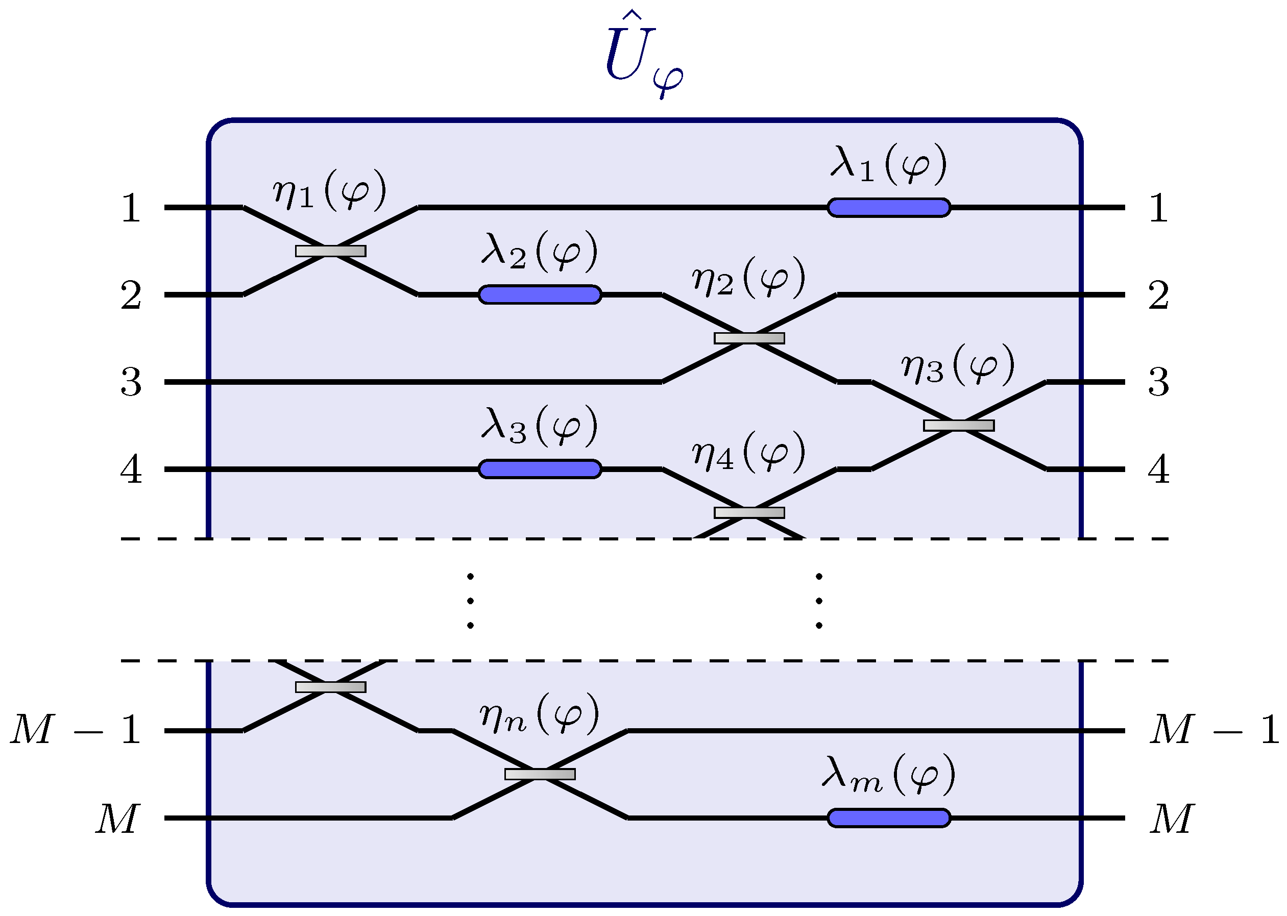
Figure 2.
Histograms of the pre-factor in Equation (13) for (left) and (right), obtained numerically with samplings of U with respect of the unitary Haar measure [36]. The generator chosen is a diagonal matrix with half 1s and half 3s as entries. The histograms are normalized to the unity. We can see that in the histogram in the right, the values of the pre-factor are more concentrated around its average .
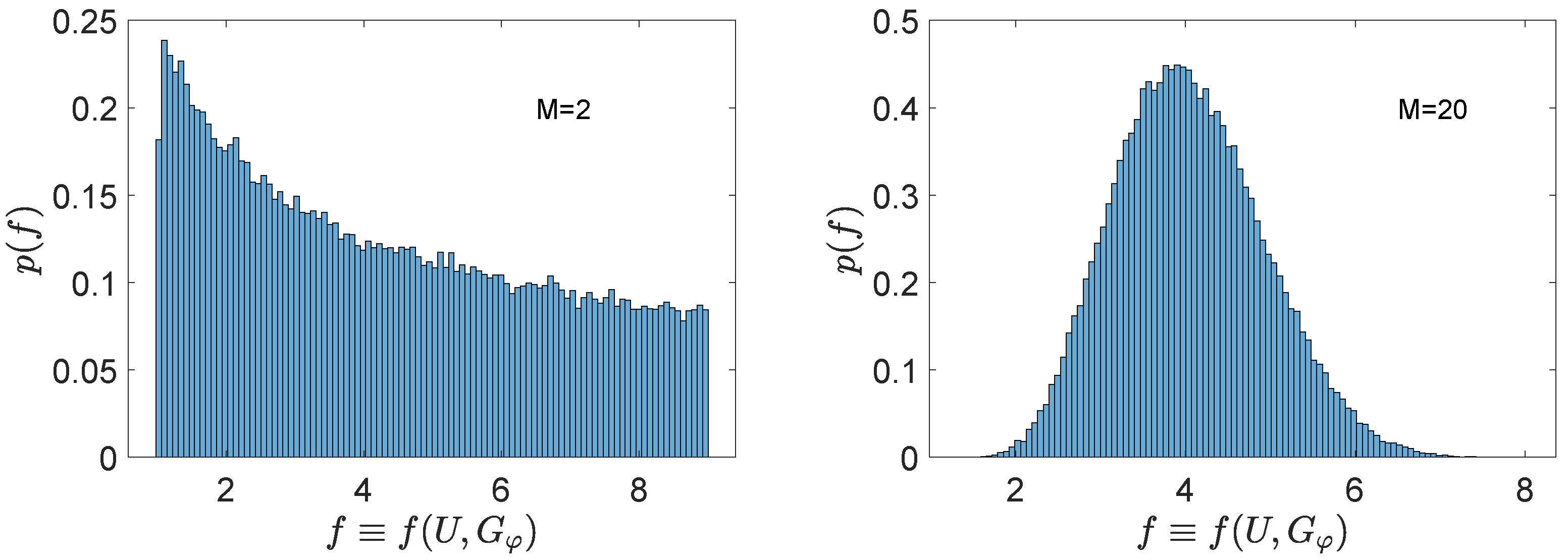
Figure 3.
Diagram of the setup described in Section 4.1 [37]. A squeezed vacuum state is injected in the first input port of a network composed of a first auxiliary stage , a linear and passive network which depends on multiple unknown parameters , and a second auxiliary stage . The two auxiliary stages are linear and passive networks whose purpose is to manipulate how the information on and on the structure of the network is encoded into the probe, and to refocus it in the only output channel observed through homodyne detection. This setup reaches the Heisenberg limit in the estimation of the overall phase acquired by the probe, which is a function of the parameters that can be manipulated through the choice of and .
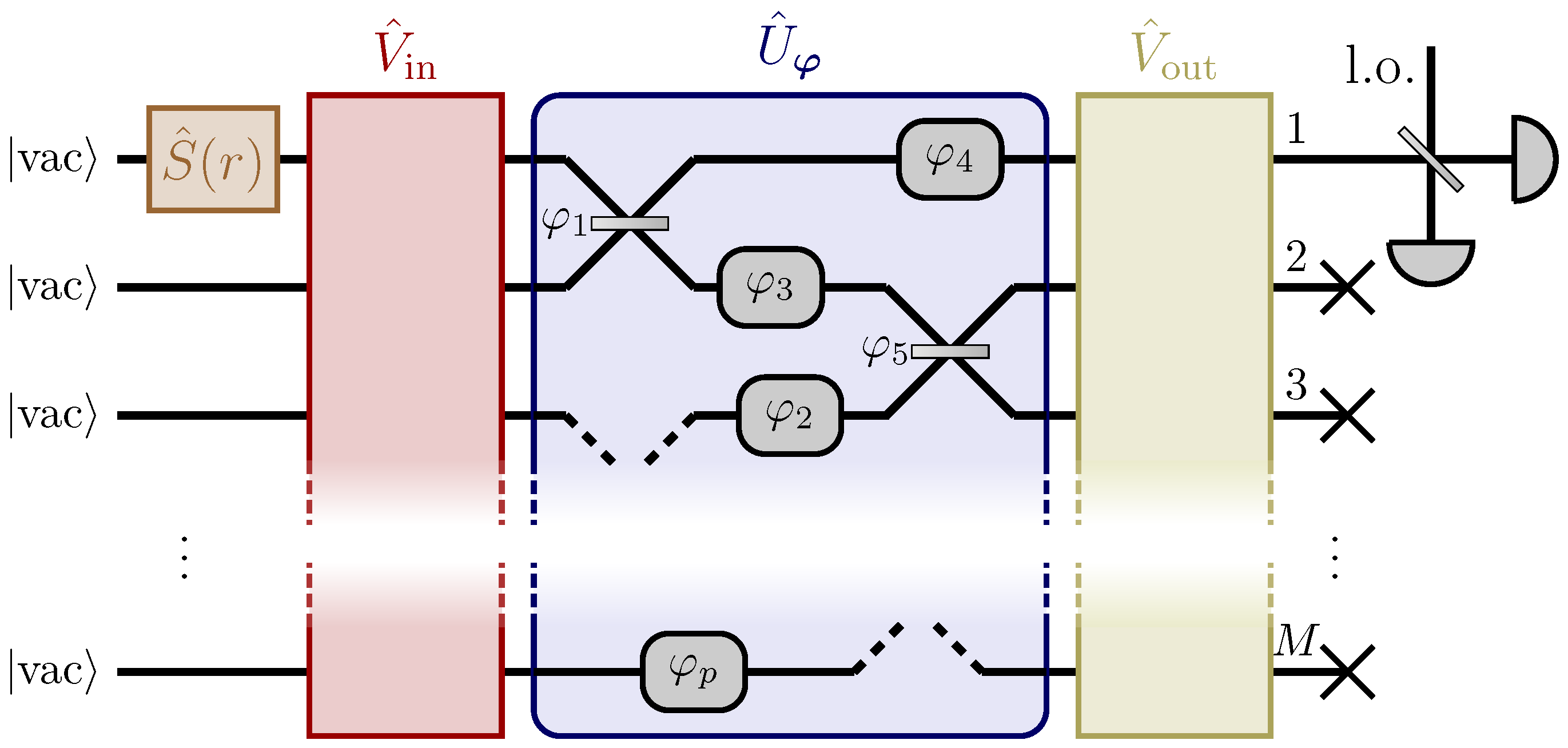
Figure 4.
A 2-channel example of a network which allows to estimate at the Heisenberg limit certain functions of the reflectivity of a beam-splitter and the magnitudes of phase-shifts [37]. The form of the function can be manipulated by changing the values of the arbitrary parameters , with (see Equation (46)), while the value of is shown in Equation (43). Similarly to the setup for the single-parameter model described in Section 2, a classical knowledge of the unknown parameters suffices to optimize the network.
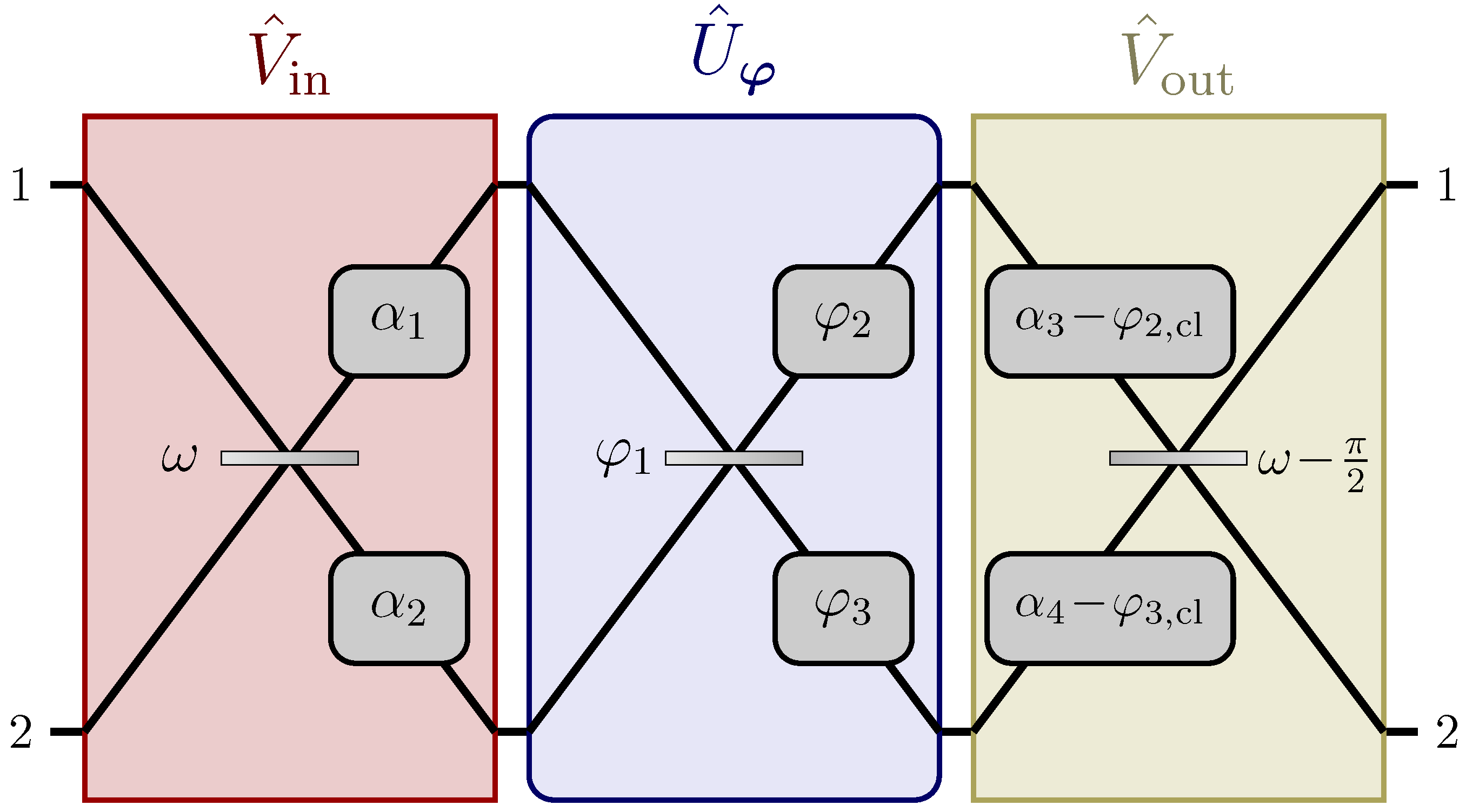
Figure 5.
Network for the estimation at the Heisenberg limit of any linear combination of M parameters with positive weights, as shown in Equation (55) [37]. As shown in the lower panel, each parameter can either be (a) an optical phase acquired through a single-mode phase-shift, or (b) the reflectivity of a lossless beam-splitter. The network (b) is given in Equation (56), and its purpose is to transform the reflectivity into an optical phase. Two auxiliary stages and are employed, whose purpose is to distribute the probe according to the weights in the linear combination (see Equation (59)), and to refocus the probe into the first output port of the network (see Equation (60)).

Publisher’s Note: MDPI stays neutral with regard to jurisdictional claims in published maps and institutional affiliations. |
© 2022 by the authors. Licensee MDPI, Basel, Switzerland. This article is an open access article distributed under the terms and conditions of the Creative Commons Attribution (CC BY) license (https://creativecommons.org/licenses/by/4.0/).
Share and Cite
MDPI and ACS Style
Triggiani, D.; Facchi, P.; Tamma, V. The Role of Auxiliary Stages in Gaussian Quantum Metrology. Photonics 2022, 9, 345. https://doi.org/10.3390/photonics9050345
AMA Style
Triggiani D, Facchi P, Tamma V. The Role of Auxiliary Stages in Gaussian Quantum Metrology. Photonics. 2022; 9(5):345. https://doi.org/10.3390/photonics9050345
Chicago/Turabian StyleTriggiani, Danilo, Paolo Facchi, and Vincenzo Tamma. 2022. "The Role of Auxiliary Stages in Gaussian Quantum Metrology" Photonics 9, no. 5: 345. https://doi.org/10.3390/photonics9050345
Note that from the first issue of 2016, this journal uses article numbers instead of page numbers. See further details here.