Coherence Stokes Parameters in the Description of Electromagnetic Coherence

Abstract

The two-point counterparts of the traditional Stokes parameters, which are called the coherence Stokes parameters, have recently been extensively used for assessing the coherence properties of random electromagnetic light beams. In this work, we highlight their importance by emphasizing two features associated with them. First, the role of polarization in electromagnetic coherence is significantly elucidated when the coherence Stokes parameters are used. Second, the normalized coherence Stokes parameters should be regarded as the true electromagnetic counterparts of the normalized scalar-field correlation coefficient.

1. Introduction

Electromagnetic description of light fields is playing an increasingly larger role in modern photonics where optical near fields and other highly nonparaxial situations involving, e.g., optical microcavities, photonic crystal elements, plasmonic structures, evanescent waves, and high-numerical-aperture arrangements are often encountered [1]. This trend also reflects the development of optical coherence theory, whose formulation within the electromagnetic domain has been active in recent years [2,3,4,5]. In the vectorial-field context, the polarization properties are the focus, and their separation from two-point coherence, which produces many interference effects, is not obvious. Insight into the connection between polarization and coherence is provided by the coherence or two-point Stokes parameters, originally introduced by Ellis and Dogariu [6] and later studied by others [7,8]. These parameters are the two-point versions of the customary polarization (one-point) Stokes parameters and they have been recently successfully used, e.g., in spatial [9,10,11,12,13] and temporal [14,15] interferometry, analysis of field propagation [16], nanoscattering [17,18], as well as with quantized light fields [19].

In this work, we aimed to emphasize the role of coherence Stokes parameters in the description of electromagnetic coherence. By considering two example situations in the electromagnetic context, Young’s double-pinhole interference, and the van Cittert–Zernike theorem, we demonstrate that the use of coherence (and polarization) Stokes parameters greatly facilitates the treatment and makes the polarization-coherence connection highly transparent. In the first case, the coherence Stokes parameters at the source plane determine the polarization Stokes parameters of the far field, whereas the situation is the opposite in the latter case. In addition, we propose that instead of the normalized coherence matrix elements, the normalized coherence Stokes parameters should be regarded as the electromagnetic counterparts of the normalized scalar-field correlation coefficient. This argument is justified by the analogous appearance of the coherence Stokes parameters and the scalar-light parameter.

2. Definition of the Coherence Stokes Parameters

Consider a random, stationary, partially polarized, and partially spatially coherent electromagnetic beam propagating along the z-axis in free space. A field realization at a point $\mathbf{r}$ and at frequency $\omega$ is given by $\mathbf{E}(\mathbf{r},\omega )={[E_x(\mathbf{r},\omega ),E_y(\mathbf{r},\omega )]}^{\mathrm{T}}$, where T denotes the transpose. The spatial coherence properties of the field at ${\mathbf{r}}_1$ and ${\mathbf{r}}_2$ are represented by the cross-spectral density matrix [2,3],

$$\mathbf{W}({\mathbf{r}}_1,{\mathbf{r}}_2,\omega )=\langle {\mathbf{E}}^{*}({\mathbf{r}}_1,\omega ){\mathbf{E}}^{\mathrm{T}}({\mathbf{r}}_2,\omega )\rangle ,$$

(1)

where the angle brackets and asterisk denote ensemble averaging and complex conjugation, respectively. The elements of this matrix are given by

$$W_{ij}({\mathbf{r}}_1,{\mathbf{r}}_2,\omega )=\langle E_i^{*}({\mathbf{r}}_1,\omega )E_j({\mathbf{r}}_2,\omega )\rangle ,(i,j)\in (x,y),$$

(2)

and electromagnetic coherence could be described using these four functions. However, an alternative and physically more transparent treatment regarding the role of polarization in electromagnetic coherence is established by using the spectral coherence (two-point) Stokes parameters [3,6,7,8]

$$\begin{array}{cc}{\mathit{S}}_0({\mathbf{r}}_1,{\mathbf{r}}_2,\omega )& =W_{xx}({\mathbf{r}}_1,{\mathbf{r}}_2,\omega )+W_{yy}({\mathbf{r}}_1,{\mathbf{r}}_2,\omega ),\end{array}$$

(3a)

$$\begin{array}{cc}{\mathit{S}}_1({\mathbf{r}}_1,{\mathbf{r}}_2,\omega )& =W_{xx}({\mathbf{r}}_1,{\mathbf{r}}_2,\omega )-W_{yy}({\mathbf{r}}_1,{\mathbf{r}}_2,\omega ),\end{array}$$

(3b)

$$\begin{array}{cc}{\mathit{S}}_2({\mathbf{r}}_1,{\mathbf{r}}_2,\omega )& =W_{xy}({\mathbf{r}}_1,{\mathbf{r}}_2,\omega )+W_{yx}({\mathbf{r}}_1,{\mathbf{r}}_2,\omega ),\end{array}$$

(3c)

$$\begin{array}{cc}{\mathit{S}}_3({\mathbf{r}}_1,{\mathbf{r}}_2,\omega )& =i\left[W_{yx}({\mathbf{r}}_1,{\mathbf{r}}_2,\omega )-W_{xy}({\mathbf{r}}_1,{\mathbf{r}}_2,\omega )\right].\end{array}$$

(3d)

These parameters appear as the coefficients when the cross-spectral density matrix is expanded as

$$\mathbf{W}({\mathbf{r}}_1,{\mathbf{r}}_2,\omega )=\frac{1}{2}\sum _{n=0}^3{\mathit{S}}_n({\mathbf{r}}_1,{\mathbf{r}}_2,\omega ){\sigma }_n,$$

(4)

where ${\sigma }_n$, $n\in \left(0\dots 3\right)$ are the Pauli spin matrices [2].

Insight into the coherence Stokes parameters is obtained by writing them in terms of the cross-spectral density functions related to specific polarization states. These are invoked by projecting the field onto the polarization state in question, i.e.,

$$W_{mm}({\mathbf{r}}_1,{\mathbf{r}}_2,\omega )={\widehat{\mathbf{e}}}_m^{†}\mathbf{W}({\mathbf{r}}_1,{\mathbf{r}}_2,\omega ){\widehat{\mathbf{e}}}_m,$$

(5)

where † denotes the conjugate transpose. The subscript $m\in (x,y,\alpha ,\beta ,r,l)$ signifies x, y, $+{45}^{\circ }$, and $-{45}^{\circ }$ (with respect to the x-axis), and the right-hand and left-hand circular polarization states, respectively. The related (complex) unit vectors are written as ${\widehat{\mathbf{e}}}_x={[1,0]}^{\mathrm{T}}$, ${\widehat{\mathbf{e}}}_y={[0,1]}^{\mathrm{T}}$, ${\widehat{\mathbf{e}}}_{\alpha }={[1,1]}^{\mathrm{T}}/\sqrt{2}$, ${\widehat{\mathbf{e}}}_{\beta }={[-1,1]}^{\mathrm{T}}/\sqrt{2}$, ${\widehat{\mathbf{e}}}_r={[1,-i]}^{\mathrm{T}}/\sqrt{2}$, and ${\widehat{\mathbf{e}}}_l={[1,i]}^{\mathrm{T}}/\sqrt{2}$. Employing the correlation functions in Equation (5) the coherence Stokes parameters become [8]

$$\begin{array}{cc}{\mathit{S}}_0({\mathbf{r}}_1,{\mathbf{r}}_2,\omega )& =W_{xx}({\mathbf{r}}_1,{\mathbf{r}}_2,\omega )+W_{yy}({\mathbf{r}}_1,{\mathbf{r}}_2,\omega ),\end{array}$$

(6a)

$$\begin{array}{cc}{\mathit{S}}_1({\mathbf{r}}_1,{\mathbf{r}}_2,\omega )& =W_{xx}({\mathbf{r}}_1,{\mathbf{r}}_2,\omega )-W_{yy}({\mathbf{r}}_1,{\mathbf{r}}_2,\omega ),\end{array}$$

(6b)

$$\begin{array}{cc}{\mathit{S}}_2({\mathbf{r}}_1,{\mathbf{r}}_2,\omega )& =W_{\alpha \alpha }({\mathbf{r}}_1,{\mathbf{r}}_2,\omega )-W_{\beta \beta }({\mathbf{r}}_1,{\mathbf{r}}_2,\omega ),\end{array}$$

(6c)

$$\begin{array}{cc}{\mathit{S}}_3({\mathbf{r}}_1,{\mathbf{r}}_2,\omega )& =W_{rr}({\mathbf{r}}_1,{\mathbf{r}}_2,\omega )-W_{ll}({\mathbf{r}}_1,{\mathbf{r}}_2,\omega ).\end{array}$$

(6d)

Therefore, six different correlation functions, each related to a different polarization state, can be used to express the coherence Stokes parameters appearing in Equation (3). The above forms have practical significance as they provide a method to measure the coherence Stokes parameters by extracting the various polarization components (with a polarizer and a waveplate) and determining the ensuing correlation function [17,18].

For ${\mathbf{r}}_1={\mathbf{r}}_2$, the coherence Stokes parameters reduce to the traditional polarization (one-point) Stokes parameters, i.e.,

$$S_n(\mathbf{r},\omega )={\mathit{S}}_n(\mathbf{r},\mathbf{r},\omega ),n\in (0,\dots ,3).$$

(7)

Thus, $S_0(\mathbf{r},\omega )$ is the total intensity, while the other polarization Stokes parameters evidently manifest the spectral density differences of the various polarization components.

Particularly important quantities are the intensity normalized coherence Stokes parameters, defined by

$${\mu }_n({\mathbf{r}}_1,{\mathbf{r}}_2,\omega )=\frac{{\mathit{S}}_n({\mathbf{r}}_1,{\mathbf{r}}_2,\omega )}{{\left[S_0({\mathbf{r}}_1,\omega )S_0({\mathbf{r}}_2,\omega )\right]}^{1/2}},n\in (0,\dots ,3).$$

(8)

As we will soon see, these functions appear in various situations involving the diffraction and propagation of random electromagnetic beams. Especially, they often play a role analogous to the scalar-field correlation coefficient, and consequently deserve to be considered its electromagnetic counterparts. In addition, the normalized coherence Stokes parameters enable writing the electromagnetic degree of coherence [5] as

$${\mu }^2({\mathbf{r}}_1,{\mathbf{r}}_2,\omega )=\frac{1}{2}\sum _{n=0}^3{\left|{\mu }_n({\mathbf{r}}_1,{\mathbf{r}}_2,\omega )\right|}^2,$$

(9)

whose value is bounded within $0\le \mu ({\mathbf{r}}_1,{\mathbf{r}}_2,\omega )\le 1$. The lower and upper limits correspond to complete incoherence and full coherence, respectively, at the two points and at frequency $\omega$.

3. Intensity and Polarization Modulations in Young’s Two-Pinhole Interference

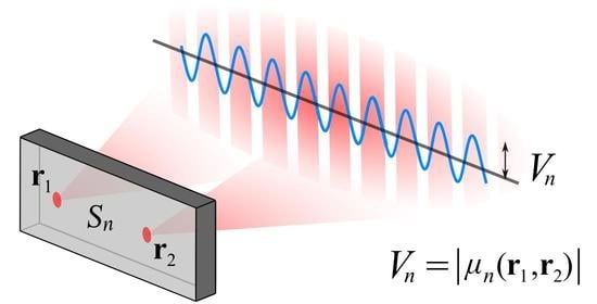
Assume a well-collimated random beam incident orthogonally on an opaque screen A, as shown in Figure 1. The screen contains two pinholes whose centers are at ${\mathbf{r}}_1$ and ${\mathbf{r}}_2$. The pinholes are assumed to be so large that the effects due to boundaries can be omitted and that the diffraction from the holes is paraxial. However, they are taken to be so small that the fields within them can be considered uniform. The interference pattern of the fields diffracted from the pinholes is analyzed near the optical axis on another screen B located several wavelengths away from the first screen.

The interference field realization on the screen B, at point $\mathbf{r}$ and at frequency $\omega$, can be written as a superposition of the spherical waves diverging from the apertures in the form

$$\mathbf{E}(\mathbf{r},\omega )=K_1\mathbf{E}({\mathbf{r}}_1,\omega )\frac{exp\left(ik{R}_1\right)}{R_1}+K_2\mathbf{E}({\mathbf{r}}_2,\omega )\frac{exp\left(ik{R}_2\right)}{R_2},$$

(10)

where $\mathbf{E}({\mathbf{r}}_1,\omega )$ and $\mathbf{E}({\mathbf{r}}_2,\omega )$ are the field realizations in the pinholes, k is the wave number, and $R_m$ with $m=(1,2)$ being the distance of the point $\mathbf{r}$ from the pinhole at ${\mathbf{r}}_m$. The parameters $K_1$ and $K_2$ are pure imaginary numbers of the form $K_m=-(i/\lambda )d{A}_m$ [2], where $\lambda$ is the wavelength and $d{A}_m$ is the area of the pinhole located at ${\mathbf{r}}_m$, $m\in (1,2)$.

The polarization Stokes parameters of Equation (7) at B can straightforwardly be written in the form

$$\begin{array}{cc}{S}_n(\mathbf{r},\omega )& =S_n^{\left(1\right)}(\mathbf{r},\omega )+S_n^{\left(2\right)}(\mathbf{r},\omega )+2\sqrt{S_0^{\left(1\right)}(\mathbf{r},\omega )S_0^{\left(2\right)}(\mathbf{r},\omega )}\hfill \\ \hfill & \times |{\mu }_n({\mathbf{r}}_1,{\mathbf{r}}_2,\omega )|cos\left\{arg\left[{\mu }_n({\mathbf{r}}_1,{\mathbf{r}}_2,\omega )\right]-k(R_1-R_2)\right\},n\in \left(0\dots 3\right),\hfill \end{array}$$

(11)

where $S_n^{\left(1\right)}(\mathbf{r},\omega )$ and $S_n^{\left(2\right)}(\mathbf{r},\omega )$ denote the Stokes parameters when the pinhole at ${\mathbf{r}}_2$ or ${\mathbf{r}}_1$, respectively, is closed. In addition, $arg\left(\alpha \right)$ denotes the phase of complex number $\alpha$. Since the observation plane B is far from the plane A, the field around the optical axis is essentially a plane wave, implying that the Stokes parameters there due to individual apertures are spatially slowly varying functions. Thus, the Stokes parameters vary sinusoidally with position owing to the term $k(R_1-R_2)$. If the intensities at the pinholes are the same, the visibilities of the Stokes parameter modulations are given by

$$V_n(\mathbf{r},\omega )=\frac{\max \left[S_n(\mathbf{r},\omega )\right]-\min \left[S_n(\mathbf{r},\omega )\right]}{\max \left[S_0(\mathbf{r},\omega )\right]+\min \left[S_0(\mathbf{r},\omega )\right]}=\left|{\mu }_n({\mathbf{r}}_1,{\mathbf{r}}_2,\omega )\right|,n\in \left(0\dots 3\right),$$

(12)

where max and min denote the maximum and minimum values of the argument function in the neighborhood of $\mathbf{r}$, respectively.

We then arrive at an important conclusion: the modulation of the polarization Stokes parameter $S_m(\mathbf{r},\omega )$ in the diffracted far field is specified by the related coherence Stokes parameter ${\mathit{S}}_m({\mathbf{r}}_1,{\mathbf{r}}_2,\omega )$ at the apertures $m\in (0,\dots ,3)$. More precisely, the magnitude of the normalized coherence parameter determines the modulation visibility and the phase affects the location of the modulation fringe pattern. Young’s interferometer therefore serves as an important example of a situation where the polarization Stokes parameters at the output are effectively specified by the coherence Stokes parameters at the input. An analogous result is also found for temporal interference in Michelson’s interferometer [14,15]. In addition, Equation (11) shows that the normalized coherence Stokes parameters play roles similar to the normalized scalar field correlation coefficient in the scalar version of Young’s interference [2]. Therefore, instead of the normalized cross-spectral density matrix elements, these electromagnetic coherence parameters should be regarded as electromagnetic counterparts of the scalar field correlation coefficient.

4. Far-Zone Form of the Van Cittert–Zernike Theorem with Stokes Parameters

The van Cittert–Zernike theorem governing the radiation from a spatially incoherent planar source is a key result of optical coherence theory [2]. Originally, it was formulated for scalar fields, showing that the source intensity determines the spatial coherence properties of the emitted field. In particular, the far-zone degree of coherence (normalized correlation coefficient) is proportional to the Fourier transform of the source intensity, a result with significant practical value. The vector-field formulation of the van Cittert–Zernike theorem was considered long ago [20] but, recently, it has attracted renewed interest by several groups [21,22,23,24,25]. Despite these significant contributions, the polarization–coherence connection included in the van Cittert–Zernike theorem is not highly transparent, since the polarization and coherence Stokes parameters are not employed. Such a formulation was given in [16], whose main findings we summarize below.

Consider a planar, partially polarized, and spatially incoherent ($\delta$-correlated) source denoted by $\sigma$ in the $z=0$ plane (Figure 2). We are interested in the far field in the paraxial regime where we can analyze the field in terms of the $2\times 2$ cross-spectral density matrix associated with the transverse x and y field components. The far field is obtained using Rayleigh’s first diffraction formula [2] and invoking the standard far-zone approximation. Employing such a procedure, the normalized coherence Stokes parameters in the far-zone points ${\mathbf{r}}_1$ and ${\mathbf{r}}_2$ take the forms [16]

$$\begin{array}{cc}{\mu }_n({\mathbf{r}}_1,{\mathbf{r}}_2,\omega )& =exp\left[ik(r_2-r_1)\right]{\int }_{\sigma }{s}_n({\rho }^{\prime },\omega )exp(-ik\Delta \widehat{\mathbf{u}}·{\rho }^{\prime }){\mathrm{d}}^2{\rho }^{\prime },n\in (0,\dots ,3),\end{array}$$

(13)

where $s_n({\rho }^{\prime },\omega )=S_n({\rho }^{\prime },\omega )/{\int }_{\sigma }{S}_0({\rho }^{\prime },\omega ){\mathrm{d}}^2{\rho }^{\prime }$ is the polarization Stokes parameter n normalized by the total intensity of the source. Furthermore, $r_1=\left|{\mathbf{r}}_1\right|$, $r_2=\left|{\mathbf{r}}_2\right|$, and $\Delta \widehat{\mathbf{u}}={\widehat{\mathbf{u}}}_2-{\widehat{\mathbf{u}}}_1$, where ${\widehat{\mathbf{u}}}_1$ and ${\widehat{\mathbf{u}}}_2$ are the unit vectors expressing the far-field directions. The equation above shows that the normalized coherence Stokes parameters of the far field generated by a spatially incoherent planar source are Fourier transforms of the corresponding polarization Stokes parameters of the source. This elegant and compact relationship shows how the different polarization components of the source contribute to the structure of electromagnetic coherence of the field. Notice that in Young’s interference arrangement discussed in Section 3 the coherence parameters at the input determine the polarization parameters at the output, but here, the situation is the opposite.

The electromagnetic-field result of Equation (13) should be compared with the corresponding scalar-field formula written as

$$\begin{array}{cc}\mu ({\mathbf{r}}_1,{\mathbf{r}}_2,\omega )& =exp\left[ik(r_2-r_1)\right]{\int }_{\sigma }s\left({\rho }^{\prime }\right)exp(-ik\Delta \widehat{\mathbf{u}}·{\rho }^{\prime }){\mathrm{d}}^2{\rho }^{\prime },\end{array}$$

(14)

where $\mu ({\mathbf{r}}_1,{\mathbf{r}}_2,\omega )$ is the normalized correlation coefficient of the scalar far field and $s({\rho }^{\prime },\omega )=S({\rho }^{\prime },\omega )/{\int }_{\sigma }S({\rho }^{\prime },\omega ){\mathrm{d}}^2{\rho }^{\prime }$ is the spectral density $S({\rho }^{\prime },\omega )$ of the source normalized with its source-integrated value. As in the context of spatial interference, we therefore conclude that the normalized coherence Stokes parameters, instead of the normalized coherence matrix elements, are the true electromagnetic counterparts of the scalar-field correlation coefficient.

5. Conclusions

In this work, we highlighted the role of the coherence Stokes parameters in the description of electromagnetic coherence. The formulation of problems involving propagation, diffraction, and interference of random vectorial light greatly benefits from the use of the coherence Stokes parameters since the effect of polarization becomes more transparent. In addition, the normalized coherence Stokes parameters often appear in places analogous to the scalar-field correlation coefficient and hence they should be considered as electromagnetic counterparts of the scalar-field concept.

References

- Novotny, L.; Hecht, B. Principles of Nano-Optics, 2nd ed.; Cambridge University: Cambridge, UK, 2012. [Google Scholar]
- Mandel, L.; Wolf, E. Optical Coherence and Quantum Optics; Cambridge University: Cambridge, UK, 1995. [Google Scholar]
- Korotkova, O. Random Light Beams: Theory and Applications; CRC Press: Boca Raton, FL, USA, 2014. [Google Scholar]
- Gil, J.J.; Ossikovski, R. Polarized Light and the Mueller Matrix Approach; CRC Press: Boca Raton, FL, USA, 2016. [Google Scholar]
- Friberg, A.T.; Setälä, T. Electromagnetic theory of optical coherence [Invited]. J. Opt. Soc. Am. A 2016, 33, 2431–2442. [Google Scholar] [CrossRef]
- Ellis, J.; Dogariu, A. Complex degree of mutual polarization. Opt. Lett. 2004, 29, 536–538. [Google Scholar] [CrossRef]
- Korotkova, O.; Wolf, E. Generalized Stokes parameters of random electromagnetic beams. Opt. Lett. 2005, 30, 198–200. [Google Scholar] [CrossRef]
- Tervo, J.; Setälä, T.; Roueff, A.; Réfrégier, P.; Friberg, A.T. Two-point Stokes parameters: Interpretation and properties. Opt. Lett. 2009, 34, 3074–3076. [Google Scholar] [CrossRef]
- Setälä, T.; Tervo, J.; Friberg, A.T. Stokes parameters and polarization contrasts in Young’s interference experiment. Opt. Lett. 2006, 31, 2208–2210. [Google Scholar] [CrossRef]
- Setälä, T.; Tervo, J.; Friberg, A.T. Contrasts of Stokes parameters in Young’s interference experiment and electromagnetic degree of coherence. Opt. Lett. 2006, 31, 2669–2671. [Google Scholar] [CrossRef] [PubMed]
- Kanseri, B.; Kandpal, H.C. Experimental determination of electric cross-spectral density matrix and generalized Stokes parameters for a laser beam. Opt. Lett. 2008, 33, 2410–2412. [Google Scholar] [CrossRef] [Green Version]
- Kanseri, B.; Rath, S.; Kandpal, H.C. Direct determination of the generalized Stokes parameters from the usual Stokes parameters. Opt. Lett. 2009, 34, 719–721. [Google Scholar] [CrossRef] [Green Version]
- Leppänen, L.-P.; Saastamoinen, K.; Friberg, A.T.; Setälä, T. Interferometric interpretation for the degree of polarization of classical optical beams. New J. Phys. 2014, 16, 113059. [Google Scholar] [CrossRef]
- Leppänen, L.-P.; Friberg, A.T.; Setälä, T. Temporal electromagnetic degree of coherence and the Stokes-parameter modulations in Michelson’s interferometer. Appl. Phys. B 2016, 122, 32. [Google Scholar] [CrossRef]
- Leppänen, L.-P.; Saastamoinen, K.; Friberg, A.T.; Setälä, T. Measurement of the degree of temporal coherence of unpolarized light beams. Photonics Res. 2017, 5, 156–161. [Google Scholar] [CrossRef] [Green Version]
- Tervo, J.; Setälä, T.; Turunen, J.; Friberg, A.T. Van Cittert–Zernike theorem with Stokes parameters. Opt. Lett. 2013, 38, 2301–2303. [Google Scholar] [CrossRef]
- Leppänen, L.-P.; Saastamoinen, K.; Friberg, A.T.; Setälä, T. Detection of electromagnetic degree of coherence with nanoscatterers: Comparison with Young’s interferometer. Opt. Lett. 2015, 40, 2898–2900. [Google Scholar] [CrossRef]
- Saastamoinen, K.; Partanen, H.; Friberg, A.T.; Setälä, T. Probing the electromagnetic degree of coherence of light beams with nanoscatterers. ACS Photonics 2020, 7, 1030–1035. [Google Scholar] [CrossRef]
- Norrman, A.; Friberg, A.T.; Leuchs, G. Vector-light quantum complementarity and the degree of polarization. Optica 2020, 7, 93–97. [Google Scholar] [CrossRef]
- Jacobson, A.D. An analysis of the second moment of fluctuating electromagnetic fields part I: Theory. IEEE Trans. Antennas Propag. 1967, 15, 24–32. [Google Scholar] [CrossRef]
- Gori, F.; Santarsiero, M.; Borghi, R.; Piquero, G. Use of the van Cittert–Zernike theorem for partially polarized sources. Opt. Lett. 2000, 25, 1291–1293. [Google Scholar] [CrossRef] [PubMed] [Green Version]
- Alonso, M.A.; Korotkova, O.; Wolf, E. Propagation of the electric correlation matrix and the van Cittert–Zernike theorem for random electromagnetic fields. J. Mod. Opt. 2006, 53, 969–978. [Google Scholar] [CrossRef]
- Ostrovsky, A.S.; Martínez-Niconoff, G.; Martínez-Vara, P.; Olvera-Santamaría, M.A. The van Cittert–Zernike theorem for electromagnetic fields. Opt. Express 2009, 17, 1746–1752. [Google Scholar] [CrossRef]
- Shirai, T. Some consequences of the van Cittert–Zernike theorem for partially polarized stochastic electromagnetic fields. Opt. Lett. 2009, 34, 3761–3763. [Google Scholar] [CrossRef]
- Rodríguez-Herrera, O.G.; Tyo, J.S. Generalized van Cittert–Zernike theorem for the cross-spectral density matrix of quasi-homogeneous planar electromagnetic sources. J. Opt. Soc. Am. A 2012, 29, 1939–1947. [Google Scholar] [CrossRef] [PubMed]
Figure 1.
Illustration of Young’s two-pinhole interference.
Figure 2.
Geometry and notations related to the van Cittert–Zernike theorem.
Publisher’s Note: MDPI stays neutral with regard to jurisdictional claims in published maps and institutional affiliations. |
© 2021 by the authors. Licensee MDPI, Basel, Switzerland. This article is an open access article distributed under the terms and conditions of the Creative Commons Attribution (CC BY) license (http://creativecommons.org/licenses/by/4.0/).
Share and Cite
MDPI and ACS Style
Setälä, T.; Saastamoinen, K.; Friberg, A.T. Coherence Stokes Parameters in the Description of Electromagnetic Coherence. Photonics 2021, 8, 85. https://doi.org/10.3390/photonics8030085
AMA Style
Setälä T, Saastamoinen K, Friberg AT. Coherence Stokes Parameters in the Description of Electromagnetic Coherence. Photonics. 2021; 8(3):85. https://doi.org/10.3390/photonics8030085
Chicago/Turabian StyleSetälä, Tero, Kimmo Saastamoinen, and Ari T. Friberg. 2021. "Coherence Stokes Parameters in the Description of Electromagnetic Coherence" Photonics 8, no. 3: 85. https://doi.org/10.3390/photonics8030085
Note that from the first issue of 2016, this journal uses article numbers instead of page numbers. See further details here.