


Abstract
Concerted rotations of a self-focused varied line-space diffraction grating about its groove axis and surface normal define a new geometric class of monochromator. Defocusing is canceled, while the scanned wavelength is reinforced at fixed conjugate distances and horizontal deviation angle. This enables high spectral resolution over a wide band, and is of particular advantage at grazing reflection angles. A new, rigorous light-path formulation employs non-paraxial reference points to isolate the lateral ray aberrations, with those of power-sum explicitly expanded for a plane grating. Each of these 14 Fermat equations agrees precisely with the value extracted from numerical raytrace simulations. An example soft X-ray design (6° deviation angle and 2 × 4 mrad aperture) attains a resolving power over a three octave scan range. The proposed rotation scheme is not limited to plane surfaces or monochromators, providing a new degree of freedom in optical design. Grating rotation about its third (meridional) axis may be employed to cancel vertical deflection of the diffracted beam while maintaining the above aberration correction. This enables a simpler (pure rotary) motion for the exit slit and a fixed beam direction both horizontally and vertically.
1. Introduction
The reflection of light at wavelengths is encumbered by losses to absorption and scattering, whose reduction favors few and simple (plane or spherical) optical surfaces. This design philosophy inspired the invention of two prior self-focusing grating monochromators suitable for use at grazing incidence [1,2,3]. The first combined rotation and translation of a varied line-space (VLS) concave grating, while the second introduced surface-normal rotation (SNR) and initially employed a constant line-space (CLS) concave grating. To date, these have been the only single-element solutions which remain “in-focus” (no spectral aberration linear versus aperture) with scanned wavelength, yet employ slit positions and ray directions fixed in the direction of dispersion. The endpoint in this progression towards minimization would be reflection from a single plane grating surface, which can exhibit near-invariance of the focal length with graze angle and provide access to the most accurate fabrication methods. These include float-polishing and Silicon crystal cleaving to produce atomically-smooth plane surfaces and short-wavelength lithographies which offer a new generation of flat-substrate gratings having ultra-low scatter and unconstrained two-dimensional line patterns [4].
Existing fixed-slit plane grating monochromators require additional (mirror) reflections to focus the incident beam or to maintain this focus as the grating is rotated to scan wavelength. For example, the classical Czerny–Turner design is theoretically free of geometrical aberrations, but requires two concave (in principle, parabolic) mirrors for collimation and refocusing [5]. Designs in which the grating is illuminated by uncollimated light require some form of effective aberration correction to maintain fixed slits upon rotation of the grating, of which five distinct geometric solutions have previously been devised: (I) a CLS grating plus a fixed concave (ideally, elliptical) mirror and a rotating plane mirror [6]; (II) a CLS grating plus a rotating concave (spherical) mirror [7]; (III) a VLS grating plus a fixed concave mirror [8,9], spherical or otherwise; (IV) a VLS grating plus a rotating-translating plane mirror [10]; and (V) a CLS grating rotating about its surface normal plus a fixed (ideally elliptical) concave mirror [3]. The cited references are the original disclosures, with the defining (minimum) optical geometries and characteristic imaging properties being unchanged in numerous reformulations, optimizations, augmentations, rebranding and other derivatives.
Presented here is a new monochromator geometry, in which a self-focusing VLS grating scans wavelength between slits at fixed distances and horizontal deviation angle, without the need for other optics. This paper reports the detailed imaging characteristics of the basic (astigmatic, single-element, plane grating) configuration, particularly the spectral resolution as a function of aperture and scan range. In Section 2, an approximate light-path formulation provides a cogent algebraic and geometric understanding of the new focusing principle (first degree correction) and derives an advantageous conjugate distance ratio to correct the spectral aberration of second degree. Section 3 introduces a rigorous general light-path formulation and Section 4 applies this to obtain the expansion equations for the present dual-rotation plane VLS grating. As analyzed in Section 5, these equations provide to an exacting degree the focusing condition, the required tilts of the object (or entrance slit) and image (or exit slit) and the lateral ray aberrations in both directions. In Section 6, these spatial aberrations are converted to the geometrical spectral resolution and are exemplified using the dimensional parameters of an ultra-high resolution soft X-ray monochromator. In Section 7, independent simulations (numerical raytracings) are performed and quantitatively compared to the light-path calculations. As the present introductory work lays the theoretical foundation on which subsidiary performance characteristics may be added, Section 8 briefly indicates some prospects for future practical enhancements. The new results disclosed in this paper, including the proposed geometry and two precise methods of deriving the component geometrical aberrations, are summarized in Section 9.
2. The Basic Scheme
Figure 1 illustrates a minimal astigmatic configuration of the proposed optical geometry. The coordinate systems are Cartesian and right-handed, with the general frame fixed in the laboratory being (). The object and image plane frames are also fixed, being perpendicular to the plane of the figure and using coordinate systems and , respectively. The coordinate system of the grating frame is , with its origin at the grating pole (P) and the -axis being coincident with the laboratory -axis (pointing towards the viewer). On the grating surface, G is a general point and E is at an extreme corner of a pole-centered rectangular aperture. The distances and are measured along the principal incident and diffracted rays, which intersect at the grating pole. There the principal angles of incidence () and diffraction () are measured relative to the grating tangent plane. Their sum is the in-plane angular deviation and their difference equals 2. Thus and is the effective graze angle.
At an initial wavelength , the grating surface normal is oriented at an angle relative to its zero order direction (for which , the grooves are oriented “in-plane” (at , thus parallel to the sagittal -axis) and self-focusing is provided by VLS positioning of the grooves. The object point , the grating pole P and the image point for define the “horizontal” plane of Figure 1, whose intersection with the grating tangent plane at its pole forms the meridional -axis. The “Gaussian” image plane is shown, which is at the focal distance for which the resulting horizontal defocus (first-degree) term at . As shown in Figure 1 and Figure 2b, the (horizontally) “paraxial” image point shall refer to the intersection of the exiting principal ray (for any ) with this image plane, being independent of the pupil coordinates (“non-aberrant”).
The scanning to longer wavelengths () consists of a conventional rotation (about the -axis) to the angle , coordinated with a second (and larger) rotation to the angle about the grating surface normal (-axis). If (as illustrated in Figure 1) the first rotation axis lies on the grating surface, it intersects a stationary grating pole which views the in-plane object point () and its paraxial image point () along principal ray directions whose projections onto the horizontal plane are fixed. The -axis rotation results in a strong defocusing of the spectral width which, as will be shown, may be canceled by the defocusing of opposite sign resulting from the -axis rotation.
Figure 1.
The Single-Element Plane Grating Monochromator (SEPGM), comprising (minimally) one grazing reflection. Coordinated on-center rotations and of a VLS grating maintain precise self-focusing as the wavelength is scanned. Projection is onto the horizontal plane, except the angle label for is viewed from a slight elevation for clarity. The extreme ray aberration (separation of the image points) is shown greatly exaggerated.
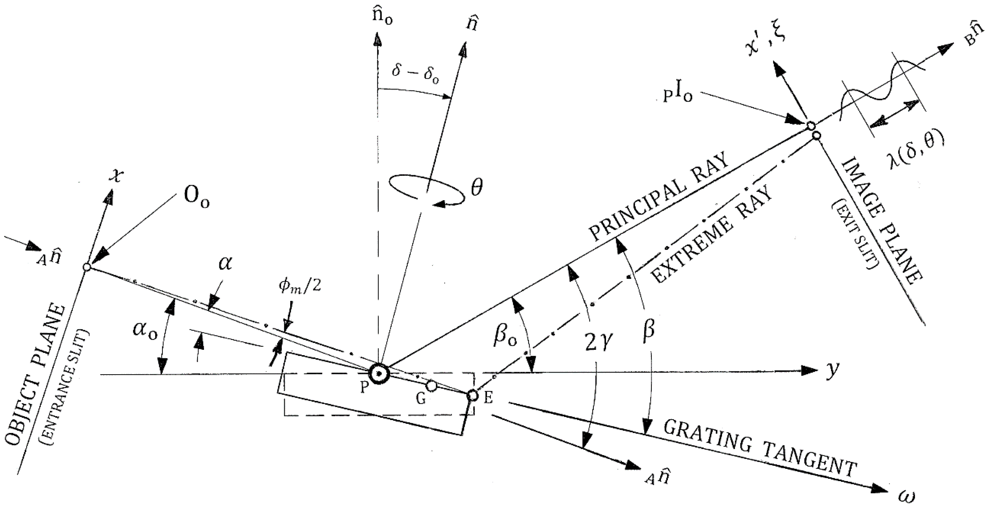
For generality and clarity, most equations will use dimensionless variables in italics, where the scale factor is r. These include the conjugate distance ratio , the meridional pupil coordinate , the sagittal pupil coordinate , the grating ruled width coordinate , the object plane horizontal coordinate and vertical coordinate , the image plane horizontal coordinate and vertical coordinate and the rotated image plane coordinates (in the spectral or “slit width” direction) and (in the “spatial” or “slit length” direction). By convention, the meridional plane is “horizontal” and the sagittal plane is “vertical”, though this directional labeling need not correspond to the ground-level orientations of either the physical instrument or the figures drawn in this paper. Meridional and sagittal shall refer to the positions and , respectively) on the grating surface, whereas horizontal and vertical shall refer to the lateral coordinates ( or and or , respectively) within the object or image planes. “Longitudinal” shall nominally refer to the direction of ray propagation. The meridional projection of the physical distance travelled by the principal ray is , which is the nominal length of the monochromator relative to the object point.
As the spectral imaging properties at grazing incidence are largely determined by the dimensionless ratio , this variable will appear in the light-path equations rather than the rotation angle . Conversion between and is given by and . The European sign convention is adopted, designating the inside spectral orders (, ) as negative () and the outside orders (, ) as positive (). Assuming no horizontal focusing optic follows the grating, and the monochromator transmits the scanned wavelength by use of a spatial filter (an exit slit), the grating image must be real (). This results in when the grating is mounted in a diverging incident beam (a real object, ), and in the case of a converging incident beam (a virtual object, ). The former corresponds to a self-focusing monochromator, for which the linear axes arrows in Figure 1 and Figure 2 point to positive dimensionless values. However in the latter case (a virtual object), the negative value of the scale factor r results in negative dimensionless values in the directions of these arrows.
2.1. The Standard Light-Path Formulation
The wavefront path length F is the sum of the physical path lengths ( and ) and the interference shift of between N grooves, where is the spectral order and is the physical value of the wavelength. As a powerful tool in the development and performance analysis of optical designs, the path lengths and groove number are usually mathematically de-composed by power series expansion in the pupil coordinates, providing (in dimensionless units):
where is the dimensionless wavelength variable given a physical line spacing at the grating pole. In what shall hereinafter be called “the standard formulation”, the path-length coefficients derive from the series expansion of the distances to conjugate points (O and I) which have no dependence upon the pupil coordinates or . In particular, I is equated to the paraxial image point . Thus, the series expansion yields equations for and which depend only upon parameters at the grating pole, namely the grating orientation (), its position () relative to the object and image points and the shape of its surface (e.g., its radius of curvature).
Employing Fermat’s principle, the image plane lateral ray positions and are also power series obtained by differentiation of Equation (1) w.r.t. the grating pupil coordinates:
where the inclination factor (given more precisely later). In Section 3, the above standard formulation of the light-path aberrations is shown to be mathematically flawed, and is replaced by a rigorously correct theory. However, to introduce the essential geometrical principles underlying the new design, this complication is temporarily neglected and a concise initial analysis is presented based on Equations (1)–(3) and other simplifying (though not flawed) approximations. For brevity, functional dependences upon the pupil coordinates and the wavelength shall hereinafter be understood without their explicit notation.
The power series terms of first degree will be referred to as de-focus (), astigmatism (), horizontal (sagittally-induced) image tilt () and vertical (meridionally-induced) image tilt (). Though semantical distractions may be discouraged by referencing the higher-degree terms according to only their (i, j) subscripts and lateral direction, the commonly accepted descriptions (based largely on the image shape) will also be used when this facilitates the discussion. Thus, “meridional coma”, “horizontal coma” or simply “coma” is the (3,0) term (), “sagittal coma”, “astigmatic coma” or “astigmatic curvature” is the horizontal (1,2) term (), “spherical aberration” is the (4,0) term () and “mixed spherical aberration” is the horizontal (2,2) term ().
2.2. Surface-Normal Rotation Transformation of the Varied Line-Space Coefficients
A varied line-space (VLS) grating is a design in which the groove positions are relatively unconstrained yet possess sufficient symmetry to permit a mechanical ruling. The most common of these symmetries is where the grooves are straight and parallel, thus the groove number (N) may be expressed as a 1D power series in the ruled width coordinate :
where and (for ) are the dimensionless VLS ruling coefficients. Equation (4) corresponds to a relative local groove density and to dimensional coefficients ).
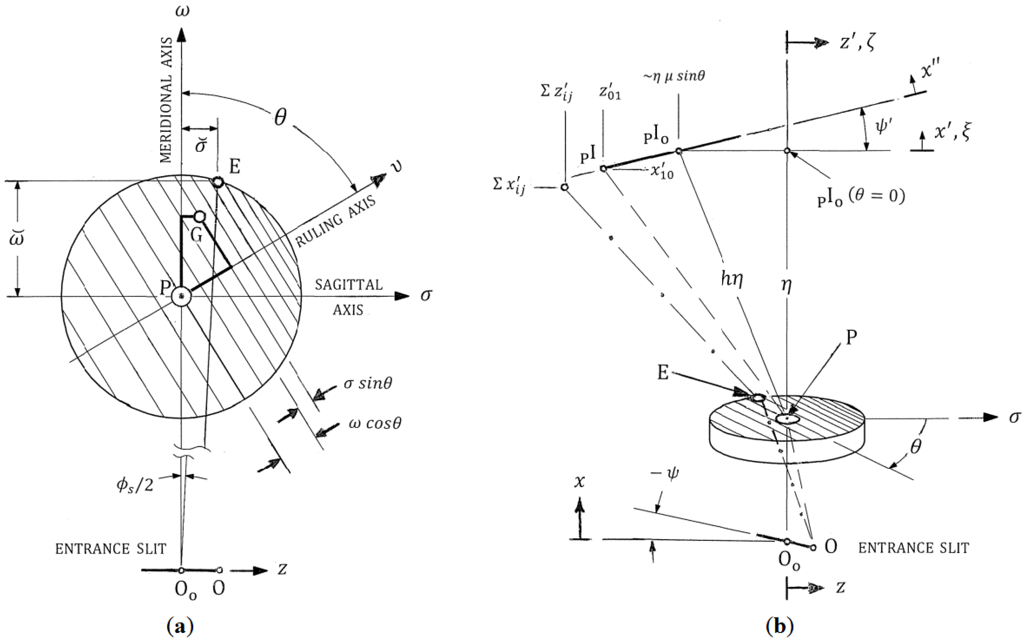
Figure 2a shows that a surface normal rotation (positive = clockwise viewed from above) of ruling coordinate relative to the grating meridional coordinate results in the transformation . The groove number coefficients in the grating frame (), as used in Equation (1), are thus obtained by that substitution in Equation (4):
where for pure meridional terms (); for pure sagittal terms (); for the mixed terms (1,1), (1,2), (2,1), (3,1) and (1,3); for the mixed term (2,2) and where . The (,0) terms provide a meridionally-projected groove density of
where revealing that the relative magnitudes between successive coefficients have decreased by . This results in diminished focusing power () and progressively smaller correction of the higher-degree aberrations (). Additionally, Equation (5) reveals that nonzero values of create new coefficients of sagittal () and mixed () powers. These new terms result in significant 3D imaging characteristics, including image tilts and the introduction of a dominant mixed aberration.
Figure 2.
(a) The grating plane viewed from above (+ ), detailing the rotational transformation of the varied line spacing between the ruling axis and the meridional axis for any point G on the grating surface, as given by Equation (5); (b) Frontal view (as seen by a distant observer upstream of the entrance slit), detailing the slit rotations in the object and image planes. The paraxial (non-aberrant) deflection out of the meridional plane is shown both originating from the center of the entrance slit (_______) and originating from one end of this slit (__ __ __ ). The (dimensionless) length of the principal ray is . The presence of aberrations, notably astigmatism, for the extreme non-principal ray (__·__) results in the lateral image position summed from all the power terms given in Section 4. Slit rotation angles (about ) and (about , given in Section 5, are relative to the grating frame. Thus, an equivalent optical geometry can maintain the entrance slit parallel to in the laboratory frame, but rotate the grating and exit slit frames by – about .
2.3. The Principal Ray Terms
These are not aberrations (pupil-dependent), but are the horizontal and vertical image coordinates, whereby the wavefront from this point to the grating pole is stationary. Using Equation (1), this condition () is expressed as:
The leading terms in Equations (7) and (8) are the differential phase shifts, namely and as given by Equation (5). The middle terms are the differentials of the object distance /r about , obtained by simple trigonometry using Figure 1 and Figure 2b (or Equations (32)–(34)) with being a point along a line (e.g., an entrance slit) tilted by an angle from the vertical. The last terms are differentials of the image distance about , also obtained trigonometrically (Equations (35)–(37)) with being the paraxial image point. Simultaneously meeting Equations (7) and (8) yields quadratics with the following series solutions:
where and . Equation (9) is a “law of sagittal reflection” with a vertical object position () and generalized to include a surface-normal rotation angle (). As illustrated in Figure 2b, the latter causes a deflection of the image center out of the horizontal plane and is dominated by the term, which scales linearly with wavelength. A possible method of canceling this (undesired) movement is proposed in Section 8.1, however this term will be included in all the aberration equations to be derived in Section 3, Section 4 and Section 5. Equation (10) is a generalized “grating equation” for the in-plane object point (, including both the projection of the groove spacing and the fine-correction factor . The result is essentially exact agreement with the numerical raytracings (discrepancy 10−13 radians). The last equality in Equation (10) is a five-term series solution which retains an accuracy of 4.2 × 10⁻¹¹ radians. Alternatively, if the term is excluded, Equation (10) is quadratic in with the following simple solution being accurate to 3.2 × 10⁻⁹ radians (~ 0.036 microns at the grating focal distance of ~ 11 meters):
In the absence of groove axis rotation, Equations (9) and (10) are found to collapse to the results reported previously for a pure surface-normal rotation monochromator [2,3], namely and . Equation (11) is the horizontal image position of off-plane points along an entrance slit, revealing that a vertically displaced object point ( results in a horizontally-displaced image point (). The term linear with corresponds to image tilt, while the quadratic term accounts for image curvature of a straight slit; further analysis is given in Section 5.4 and Section 5.5.
2.4. Pure Meridional Aberrations and their Graze Angle-Invariant Approximation
Using the paraxial horizontal image position ( to construct the path lengths and neglecting the effect of off-plane vertical image positions (), the grating Equation (10) simplifies to and the lowest three meridional-only () wavefront terms of Equation (1) may be written concisely in the following form:
where and . At grazing angles (15°), the small-angle approximations and ) provide accuracies 1%. This yields , and a simplified (-invariant) expression for the wavefront:
at nonzero spectral orders (). At the initial wavelength (prior to scanning), and and all horizontal aberrations vanish () by choice of the following VLS coefficients:
As the geometrical imaging properties of VLS plane gratings contrast with intuitions fostered in classical optics, it is emphasized that the required coefficients are (for all ) nearly independent of at grazing incidence, with this invariance becoming (asymptotically) exact as approaches zero. This is opposite to the behavior of classical (curved surface) methods of focusing, which are strongly dependent on a precise at grazing incidence, and become increasingly so as decreases. As with the prior VLS self-focusing plane grating geometry (IV in Table 1), this invariance enables a given grating to provide aberration correction at any graze angle given fixed values for , . This offers a flexibility in graze angle and wavelength coverage not available with concave gratings.
For the author’s original VLS plane grating converging-beam geometry (III in Table 1), the conjugate distance ratio is , simplifying Equation (15) to (dimensionally, this is ). Though this grating mount requires a horizontal focusing mirror to provide the incident converging beam, Equation (14) with reveals the yet stronger -invariance whereby the aberration correction is also independent of . This allows the angles of incidence and diffraction to be changed independently (while still maintaining the fixed focal length ) given only that the dimensional factor is unchanged. For example, the grating may be configured with this mirror into an erect-field (varied ) spectrograph [8] with fixed , a constant-deviation (fixed ) monochromator [9] or any other desired combination of the 2 angles. A derivative of this geometric class (i.e., having unaltered imaging properties) thus provides a fixed difference for “on-blaze” diffraction efficiency to a moveable slit (or add a conventional rotating plane pick-off mirror to redirect this to a fixed slit).
However, when (), the focal length is a strong function of . This sensitivity is a general characteristic of a self-focusing grating geometry at grazing incidence, whether it be a classical or VLS grating, and whether the surface is plane or curved. In contrast, it has been previously shown [2,3] that a surface-normal () rotation does not change the focal length of a CLS grating, given fixed meridional angles and a fixed axis-symmetric (e.g., plane or spherical) surface curvature. However, in the case of a VLS grating, an -rotation angle diminishes the interference term by the factor , as seen in Equation (14). This would result in an under-correction of all aberrations initially corrected at . The new focusing condition presented here arose by considering if this under-correction could balance the strong defocus induced by the change to upon a conventional (groove axis) rotation.
2.5. The New Focusing Condition
Combining Equations (14) and (15) in the case of no defocusing () yields:
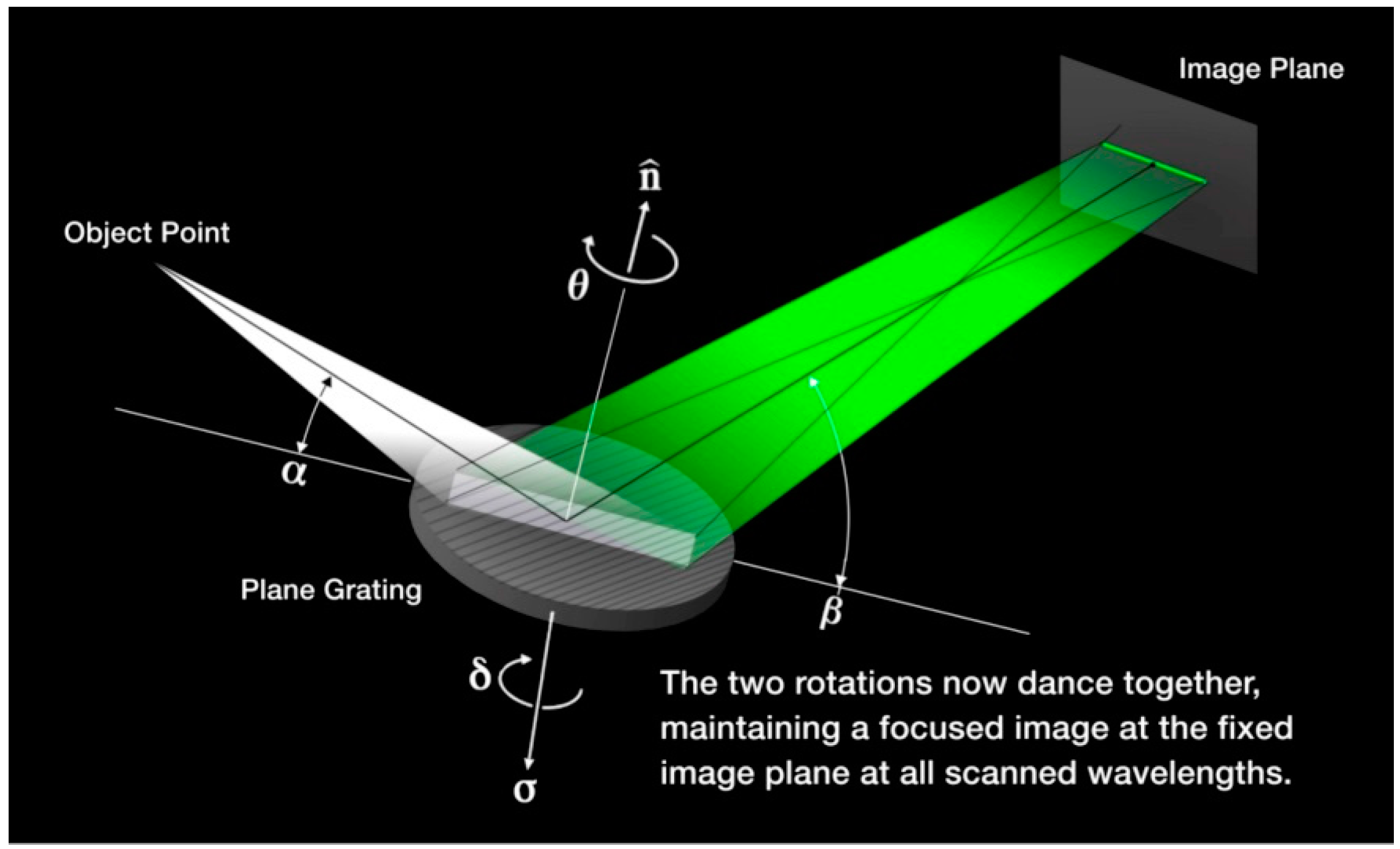
As , Equation (16) provides a mathematical relationship between the two rotation angles ( and ). However, this is of no physical relevance unless . Fortuitously, this is always the case, as may be seen by making the substitution . Equation (16) is then rewritten as . For negative spectral orders, and a scan towards longer wavelengths requires . Since in the present (self-focusing) geometry, the value of this equation must be between 0 and +1. By the principle of optical reversibility, this must also be the case for positive orders, for which the photon reverses its direction of travel and becomes 1/. The potential to cancel the defocusings induced by each of the 2 rotations (the 2 terms in Equation (14)) may also be understood geometrically. As illustrated by the first animation sequence of Figure 3, scanning towards longer wavelengths (shown visually going from “blue” to “orange”) by a -axis rotation always decreases the focal length. However, due to the cos reduction in VLS focusing power, the -rotation (away from ) always increases the focal length.
Though Equation (16) relies upon the small-angle approximation and also accounts only for pure horizontal defocusing (the effect of image tilt is addressed in Section 5), it confirms the physical relevance of this scheme. Additionally, it provides some insight by considering the case of unit magnification at . By use of Equation (16) and the small-angle approximation to the generalized grating Equation (10), the in-plane rotation and the surface-normal rotation are each seen to increase the scanned wavelength by the same amount. In the more general cases of or (away from ), though the contributions are not equal they are comparable, thus the scanning range () scales approximately as the square of that provided by each rotation. Due to this (second) fortuity, the proposed dual rotation is not only the key to a focused single-element plane grating monochromator, but also enables a wider scan in wavelength than does a single rotation for the same change in (the latter affecting grating imaging, magnification and efficiency). For the monochromator parameters exemplified in Section 2.6, a factor 8 in scan range results from a factor 2.54 due to the in-plane rotation (changing by only a factor of 1.89) times a factor 3.12 due to the surface-normal rotation.
Figure 3.
Concerted rotations of a varied line-space (VLS) self-focused plane grating about two axes provide in-focus scanning of the wavelength (please see the animation of this figure in the supplementary material). Tilt and off-plane deflection of the image are not shown here. Slits may be placed at the object and image.
2.6. Two-Point Coma-Correction: Optimization of the Conjugate Distance Ratio
With defocusing eliminated at all scanned wavelengths, the next higher degree aberration to be considered is given by in Equation (1). At grazing angles, this aberration is typically large and thus determines whether a system which is technically “in-focus” () can in fact deliver high resolution at a usable aperture. It is tempting to first consider unit magnification , which would eliminate this aberration in the absence of a varied line-density term . This is similar to the classical concave grating being free of this aberration on the (unit magnification) Rowland circle. Setting 0 would also remove this interference term from Equation (14) and thus avoid its multiplication by cos2 (which would re-introduce coma upon surface-normal rotation). However, because and are changing in opposite directions as the wavelength is scanned in the first (groove axis) rotation, the resulting change in ρ ~ β/α allows 1 at only one wavelength. Even if this correction wavelength is optimally selected (by choice of alone) to be near the center of the scanned spectrum, the growth in coma away from a single correction point is rapid, making it ineffective for all but a very narrow wavelength range.
The high level of coma correction required to maintain ultra-high spectral resolution over wide scanning ranges is realized by determining optimal values for the two free parameters ( and ) available from Equation (14) when to correct at two wavelengths. In general, the simultaneous solution is a quartic, however it collapses to a quadratic if the two correction points are (tentatively) chosen to be at (cos) and 60° (cos), resulting in the following closed-form solution:
The corresponding is obtained by setting in Equation (14) at and . Minimization of over the scan range is then obtained by adjusting both and from these tentative values, such that the two correction points straddle the spectrum center and are symmetrically inset from the edges. In this case, reaches the same maximum at the extreme ends of the range and at a wavelength between the 2 correction points. Such optimization for a scanning range of ~ 8 ( ~ 71.25°) resulted in 1.275 and 1.08 (if the scan range were reduced to ~ 60° ( ~ 3.6), optimization of this coma-correction would yield and 1.04). This and the preceding meridional analysis provide the following set of dimensionless parameters for an example soft X-ray SEPGM: 2 6°, 1.4458939, 3.699998982,1.432972878, 0.8378590, 1.28655, where results from using Equation (14) to cancel spherical aberration () at , thereby minimizing its average magnitude over the three-octave scan range.
2.7. A Classification of Plane Grating Geometries
The simple form of Equation (14) also enables a concise comparison of the fundamental differences between various aberration-corrected plane grating geometries. In Table 1, the present class is listed alongside the previous five, comparing the defining categories of the minimum number of reflections (grating + mirror(s)), the grating line density function (the VLS coefficients ), the functional value of defining the grating mount, the grating parameter which is fixed upon a focused (0) scan of wavelength and the corrected horizontal aberrations (0).
Table 1.
Plane grating aberration-corrected monochromators with fixed slits.
3. A Rigorous Theory of Light-Path Expansion
The purist of wave aberration methods [11] constructs the physical light-path from object point to actual (floating) image point and employs Fermat’s principle by setting the wave aberration differential to zero for the sum of all terms. This approach does not evaluate the individual aberrations, other than those of lowest degree in each direction (i.e., defocusing and astigmatism). This avoids the difficult task of constructing an accurate reference wavefront, and is convenient for optimizing (“fine-tuning”) the parameters of existing geometries by minimizing the numerical variation in the image point position as the incident ray wanders over the pupil surface. Unfortunately, this provides little intuitive information conducive to algebraic or geometrical understanding, and is therefore not suited to the development or qualitative improvement of new geometries. Indeed, even the (numerical) data from the precise raytracings performed as part of the present work (Section 7) are mathematically reduced to extract the individual coefficients of the algebraic power series, and are thus more convenient for basic design development than is the total wave aberration formalism.
More insight and fundamental progress in optical design is facilitated by isolating and controlling successive expansion terms (and ) of the lateral ray aberrations. Especially in the case of large mixed terms (neither i nor j being zero), this requires a more rigorous light-path formulation than previously presented in the literature. Though complicating the derivation, the resulting separation of the individual terms provides a precise and consistent analytical method indispensible to the development of new designs. In this section, the general equations are given for rigorously expanding the lateral aberrations of a reflection grating. In Section 4, these will be simplified for the case of a plane grating and used to obtain the explicit aberration terms for the basic astigmatic configuration of the new monochromator geometry.
3.1. Flaw in the Standard Theory
Relative to any chosen point in space, the optical wavefront (a surface of constant phase) is a (physically) measureable quantity, as is the lateral image position of a ray diffracted from any point on the pupil. However, their expansion into power series component terms is (though very useful) only a mathematical abstraction. In expanding the image path length relevant to an individual ( or ) lateral aberration term, a consistent formulation requires the use of a correspondingly abstract reference image point. This must be chosen to remove the other lateral aberration terms which, upon expansion and pupil differentiation of the light-path, may erroneously form the same power dependence as the intended term. Only in this way do the (mathematically-constructed) terms become separate incremental components, the sum of which is the total (physical) aberration.
In general, the reference point depends not only upon the (i, j) term in the light-path function, but also upon whether a given (i, j) term is differentiated relative to the meridional pupil coordinate to determine (via Fermat’s principle) the lateral ray position or relative to the sagittal pupil coordinate to determine . Thus, a single light-path function may not be expanded (e.g., into a power series) applicable to both directions. Nonetheless, the individual derivatives () of the appropriate functions may be expanded for rigorous determination of the separate lateral ray positions, as given in Section 3.3.
Unfortunately, the standard formulation (briefly summarized in Section 2.1) systematically employs only the paraxial image as the reference point (in wavefront terminology, it is usually asserted to use the “Gaussian reference sphere”). The resulting expanded (inferred) power terms are therefore subject to cross-contamination, providing incorrect results for both the individual aberrations and their sum, the latter thereby not matching the actual (measurable) lateral ray position. In the analysis of classical optics, such contamination is usually small, due to these designs either being rotationally symmetric, having an in-plane dispersion geometry, or being anastigmatic and (ideally) absent of second-degree (e.g., meridional coma) lateral aberrations, and is neglected. An historical exception appears to have been in determining the mixed power term of astigmatic coma (), where Beutler [12] correctly added the aberration of astigmatism () to form the image reference point for a concave grating geometry (particularly on the Rowland circle). Though such special consideration of the lowest-degree vertical aberration is consistent with the image reference being “paraxial”,
it contradicts the assertion that the wave aberration is evaluated at the (single point) intersection of the principal ray with the (horizontal) Gaussian image plane [13]. As astigmatism separates the horizontal and vertical image planes, the actual wavefront becomes toroidal. Moreover, inclusion of this one aberration in the reference does not provide a correct determination of all the lateral aberrations.
In the more general sense, this approach leaves uncorrected an underlying problem that the standard formulation is based on the methods developed for the treatment of normal incidence and rotationally symmetric classical optics systems. For such, the horizontal and vertical image planes coincide, neither astigmatism nor coma exist when using an on-axis object point and a single light-path function may be used to determine the lateral aberrations in both directions. Using such methods, the lateral terms which can dominate grazing incidence and asymmetrical systems are not systematically removed from the expansion of higher-degree aberrations. The neglected terms include all of the pure meridional aberrations (such as horizontal coma) and the mixed terms (in which both i and j are nonzero). Though a comprehensive discussion of the errors resulting from widespread use of the standard formulation is beyond the scope of this paper, Appendix A shows that the standard result for the spherical aberration term of even a (classical) spherical mirror is incorrect at non-unit magnification. This illustrates that the new formulation yields more accurate results even in the absence of surface-normal rotation, varied line-spacing, grazing incidence or even grating diffraction.
The light-path expansion theory developed below reveals that the isolation of different power series terms is generally more complex than previously explained by use of paraxial reference points. The new formulation employs a pupil-dependent (“aberrant”) reference image position tailored to the expansion of each power term, and a Fermat differentiation of infinitesimal pupil variables ( and ) which are independent of this image position and the pupil coordinates ( and ).
3.2. The Reference Path Lengths
The reference path-lengths are () as the distance between a reference point () in the object plane and the grating pupil coordinate (), and () as the distance between () and a reference point () in the image plane. The general equations in this section include a grating surface of revolution with a radius of curvature at the pole, where is concave (positive focusing power) and is convex (negative focusing power). In the below equations, provides the exact results for a paraboloidal surface, while a spherical surface is treated (correct to the 5th degree in path-length) by substituting . Given the coordinate systems shown in Figure 1 and Figure 2:
in which is the sum of the squares of the two lateral (”transverse”) segments:
where,
In Equation (19), is the vertical distance of an object point from the horizontal (meridional) plane. The terms and have no dependence upon the grating pupil coordinates and thus define a source point whose emitted rays fill the grating aperture. Making a function (or vice-versa) can define the two-dimensional curve on which such points may lie in the object plane. For example, a parabolic entrance slit illuminated by a spatially diffuse upstream source may be specified by where is the slit’s tilt angle towards the -axis and is its curvature radius at . In the case of a linear slit 1/; if is also zero, then the slit is aligned with the vertical -axis. Equations (19) and (20) also allow power series terms () to accommodate dependences between the object point position and the grating pupil position. For example, consider a vertically aligned entrance slit being illuminated by a horizontally aligned linear source at an upstream distance Y. This longitudinal separation of the effective horizontal and vertical object conjugate planes results in ). Nonzero values for or can also be constructed to include the geometrical aberrations of optics preceding the grating (or the object plane), e.g., those of a mirror which reduces the (vertical) astigmatism and/or provides horizontal re-focusing of a distant source.
The coordinate system of the image plane has as its origin the principal ray position for the in-plane configuration, namely where the object point is at ) and where the grating rotation angle 0. However, all other object points and all nonzero values of will result in an image position which does not strike this origin in one or both lateral directions. Therefore, and ), where the superscript denotes the component due to aberrations. In the case of the minimal astigmatic configuration of the SEPGM geometry (whose detailed expansion is given in Section 4), the aberration terms assume an object at ). This constrain for all rotation angles, thus contains only the aberration terms (). However, when as given by Equation (9). Thus, is the sum of an aberration component () and the off-plane position of the principal ray.
3.3. Fermat Derivation of the Lateral Ray Aberrations
Mathematical separation of the individual aberration power terms requires strict adherence to Fermat’s principle, which specifies the light-path (i.e., the direction along which the optic provides constructive interference) to be the one for which the phase is stationary relative to small offsets in the pupil coordinates. Deviations from this can be converted to the lateral ray deviations (aberrations) from a reference image point. In mathematical terms, the first derivative must be taken relative to the pupil coordinates, while maintaining a fixed reference image point. To insure a proper formulation, it is therefore convenient to add small offsets ( and ) to the two pupil coordinates ( and ) appearing in Equations (19) and (22), but not to the pupil coordinates appearing in Equations (20) and (23). The Fermat derivatives of Equations (18) and (21) are then taken with respect to and . In the absence of these effectively separate variables, i.e. if one simply differentiated with respect to and , any aberration (a ray position which depends on the pupil coordinates) included in the construction of the reference image point would move that point during the differentiation, improperly distorting the (spherical) reference wavefront. The same situation occurs in the presence of an aperture-dependent object position (discussed in Section 3.2).
The proper formulation of Fermat’s principle thereby yields:
The reference coordinates and in the above equations are each sums of all the other lateral ray aberration power terms and , respectively, which when combined and expanded with the other terms give rise to the desired power term.
The reciprocal radicals in Equations (24)–(27) are to be expanded by Taylor series (to isolate the different power terms. The horizontal lateral aberration is obtained by Fermat conversion of the wavefront error by summing the terms, retained in the -derivatives of the three path-length components (N, A and B), and multiplying by the “lever arm” distance to the image :
where,
and is the inclination factor due to an off-plane image coordinate of . As is thereby the distance between the optic center and the paraxial image point, this conversion is accurate to order , as given by Born and Wolf [14]. The trailing term in Equation (29) accounts for the linear variation of 1/sin with when the optical surface is not flat ().
For the vertical ray aberration (summing the terms), the inclination factor enters a second time at the exit pupil (in the same manner as the 1/sin factor in the horizontal equation) and a third time in projecting the transverse aberration (normal to the direction of propagation) onto the image plane. This results in a net factor of h3 , as employed below:
where,
The above general equations provide the foundation for an accurate mathematical decomposition of the lateral ray aberration into power terms (horizontally) and (vertically). The improvement over the standard formulations lies in the systematic inclusion of all other relevant (i.e., able to form expansion terms of power (horizontally) or (vertically)) aberrations and in constructing the reference image point ( for calculation of the geometrical path lengths used in determining both and .
One could integrate Equations (29) and (31) to form “wavefront” (path-length) coefficients; simply being Equations (2) and (3) in reverse, yielding for the horizontal direction and for the vertical direction. Though such an exercise adds no new information, it confirms that the individual terms in the decomposition of the wavefront (and thus lateral ray positions) are mathematical abstractions. If they were physical quantities, then and would not “know” the direction in which they may be differentiated and thus would be equivalent (). However, for the present astigmatic design, the required reference point () for is different from that for at all (i, j) pairs (see Table 2). Thus, for all i and j (when i + j 1), indeed with the ratios calculated to be of significant magnitude (102 to 103).
4. The Aberration Equations for an Astigmatic Plane Grating Monochromator
In this section, the lateral aberration terms of “power-sum” (i + j − 1)1, 2 and 3 are explicitly expanded for a planar () grating surface.
4.1. The Fermat Derivatives
Setting the curvature radius to infinity simplifies Equations (19), (22) and (24)–(27) to the following:
where,
where,
For the lateral aberrations, the expansions will use the in-plane object point . The resulting series from Equations (32) and (33) are the same as those of the standard light-path formulation:
Due to the symmetry imposed by the in-plane object, there are no odd powers of in Equation (38) and no even powers of in Equation (39).
Expansion of Equations (35) and (36) is considerably more involved, due to the presence of an image reference point (, ) whose components, as given by Equation (23), are themselves power series in both and . Equation (29) provides nine aberration terms in the horizontal direction and Equation (31) provides nine aberration terms in the vertical direction ). For a given frontal aperture aspect ratio (), the surface aperture ratio () scales linearly with the graze angle; the aberrations thereby progressively decrease in magnitude within the nth-degree power-sum family along the sequence . Thus, unless , the least-significant horizontal terms are , and the least-significant vertical terms are those which contribute to the same spectral width terms ) following the image plane rotation given in Section 6. Being exceedingly small for the example monochromator (quantitatively verified by the raytrace extraction equations given in Section 7), these four terms are not explicitly expanded here. Each of the remaining 14 aberrations employs image path-length derivatives derived from a dedicated reference image coordinate pair () summed from the other (non-(i,j)) lateral aberrations. The resulting expansion coefficients of in Equation (35) and in Equation (36) complete the determination of the Fermat-generated horizontal and vertical ray aberrations given by Equations (29) and (31), respectively.
4.2. The Explicit Expansion Terms of Power-Sum
In accordance with the detailed manual algebraic procedures exemplified for the term in Appendix B, the 14 aberration power series coefficients are given here in explicit form, following a re-listing of the three Equations (12), (9) and (11) derived in Section 2.3 for the principal ray:
where the substitute variable is of order unity at grazing incidence. While the principal ray Equations (9) and (11) include the off-plane () coordinates of a tilted entrance slit (, the effect of slit length on the aberrations is negligible at present (cf. the solid and dashed line profile raytracings in Figure 6), thus Equations (41)–(54) do not include any -components.
A summary of the accuracy provided by Equations (41)–(54) is given in Table 2, using the ultra-high resolution soft X-ray monochromator (parameterized at the end of Section 2.6) as a test case. The RMS deviations between these light-path equations and independent numerical raytrace simulations (Section 7) are given in the last 5 columns. Also listed are the lateral rays, including aberrations, which form the reference image position . The top-down sequence in this table provides the terms needed for the reference image in subsequent expansions. The bracketed {terms} and corresponding {errors} in the S.F. column refer to the standard light-path formulation {paraxial reference image, including astigmatism per Section 3.1}.
Table 2.
Reference image lateral positions and residual calculation errors.
As listed in Table 2, the reference points for the highest-degree mixed terms () include numerous lower-degree aberrations and were therefore undertaken only for the linear sub-term in . These terms provide the worst accuracies (0.02 microns laterally at the image plane), albeit of no practical significance at present. All the other aberration terms were expanded to include the powers in needed to decrease the lateral errors to the size of an atom (0.001 microns) or below, insuring they will endure any conceivable future physical application.
By comparison, the standard light-path expansion causes significant formulation errors. This may be seen by the defocus term resulting from use of only the paraxial point in forming the reference image:
Due to the neglect of the aberration in forming the image reference position, the sub-term in this equation differs significantly from that in the rigorous Equation (44). This results in the calculation error of 93 microns listed in Table 2. As shown, there is a similar calculation error resulting from the standard formulation of the term:
This is due to neglecting three relevant aberrations () in forming the reference image. While the above equation lists only the first sub-term (linear with ), those of degree and were also generated but made little improvement due to the linear term already being flawed.
5. Manipulation and Analysis of the Ray Aberrations
5.1. Horizontal Tilt (Sagittally-Induced)
The lowest-degree mixed horizontal aberration created by the surface-normal rotation is (Equation (42)) resulting from the nonzero value of in Equation (5). Noting the linearity of with the sagittal pupil coordinate , this is simply a tilt of the astigmatic image by the angle /) about the image coordinates (0, Employing the expansions given in Equations (41) and (42):
where a negative value is counter-clockwise for an upstream observer. As in the case of the single-rotation “pure” SNR monochromator [2,3], a sympathetic rotation of the exit slit by about will cancel the rotated value of and thus . A stationary rotation axis would require adjusting the focusing condition (not detailed here) to include the horizontally offset image center intercepting the slit.
5.2. Vertical Tilt (Meridionally-Induced) and the Rigorous Focusing Condition
Given the above astigmatic image tilt, the lowest-order mixed vertical aberration presents the interesting condition that a perfect horizontal focus for meridional rays () would be extended into a vertically extended line, projected upon the tilted slit as a defocus normal to its length (multiplied by tan). In effect, the vertical aberration due to the meridional rays induces a second tilt angle . Employing Equations (43) and (44):
The solution is to purposely “defocus” the grating horizontally to force equality of the two tilts (Equations (55) and (56)). Making the following substitutions: , and constrains the single parameter to provide the following rigorous focusing condition:
accurate to order , where is a small quantity (of order ) and where at present (the terms involving are derived in Section 5.3). If one drops the and terms, a quadratic emerges whose closed-form root :
Note that the linear approximation to Equations (57) or (58) has the even simpler solution , being a pure horizontal focus ( independent of the image tilt. In the small-angle approximation, this is equivalent to that previously given by Equation (16).
The final solution for is obtained by numerical iteration of Equation (57) using the above “initial guess” of or . Even at the maximum rotation angle of , only a small adjustment in is needed to provide the desired condition . If using as the initial guess, the residual is negligible (10−12) after only 2 linear interpolations, refining by 0.064°.
Equalizing the two image tilts of a point source is critical to providing fine spectral resolution at high rotation angles. In the absence of such a constraint (i.e., if the horizontal defocus alone is corrected), the net resolution of the example monochromator is calculated to degrade by a factor 6 at
5.3. Balancing of Spherical Aberration and Defocus
Though typically a very small correction, a fine adjustment in may also be employed to partially balance the spherical aberration term. This is analogous to the classical technique of offsetting the detection plane from the Gaussian () focus to the plane of “least confusion” which minimizes the sum of these two lateral horizontal aberrations of odd power (. Unlike the defocus term, the aberrations of high power (including the term) vary only slowly with (except near their correction points). This allows the term to be evaluated at the root of Equations (57) or (58) and to then be treated as a constant to be added to for a refined determination of the meridionally-induced tilt angle () given above. For example, evaluating at from Equation (58), the full focusing condition shown in Equation (57) employs a nonzero value for and the following constant approximated by the dominant lowest-order () term of Equation (51):
An optimized balancing of defocus and spherical aberration employs of the semi-meridional aperture, resulting in the root of changing by −0.0067° at the scan wavelength of , and the extremum convolution of all the aberrations decreasing by 30% (cf. Figure 6g,h). More substantial improvements are expected at larger apertures, where spherical aberration is increasingly dominant over the lower-power aberrations.
5.4. Rotation of the Entrance Slit
Given an entrance slit at angle to the vertical, its image tilt derives simply from Equations (9) and (11):
To maintain focus along the slit length, this must be set equal to the image tilt for a point source from Equation (55). Thus, , constraining as a function of the scan parameters:
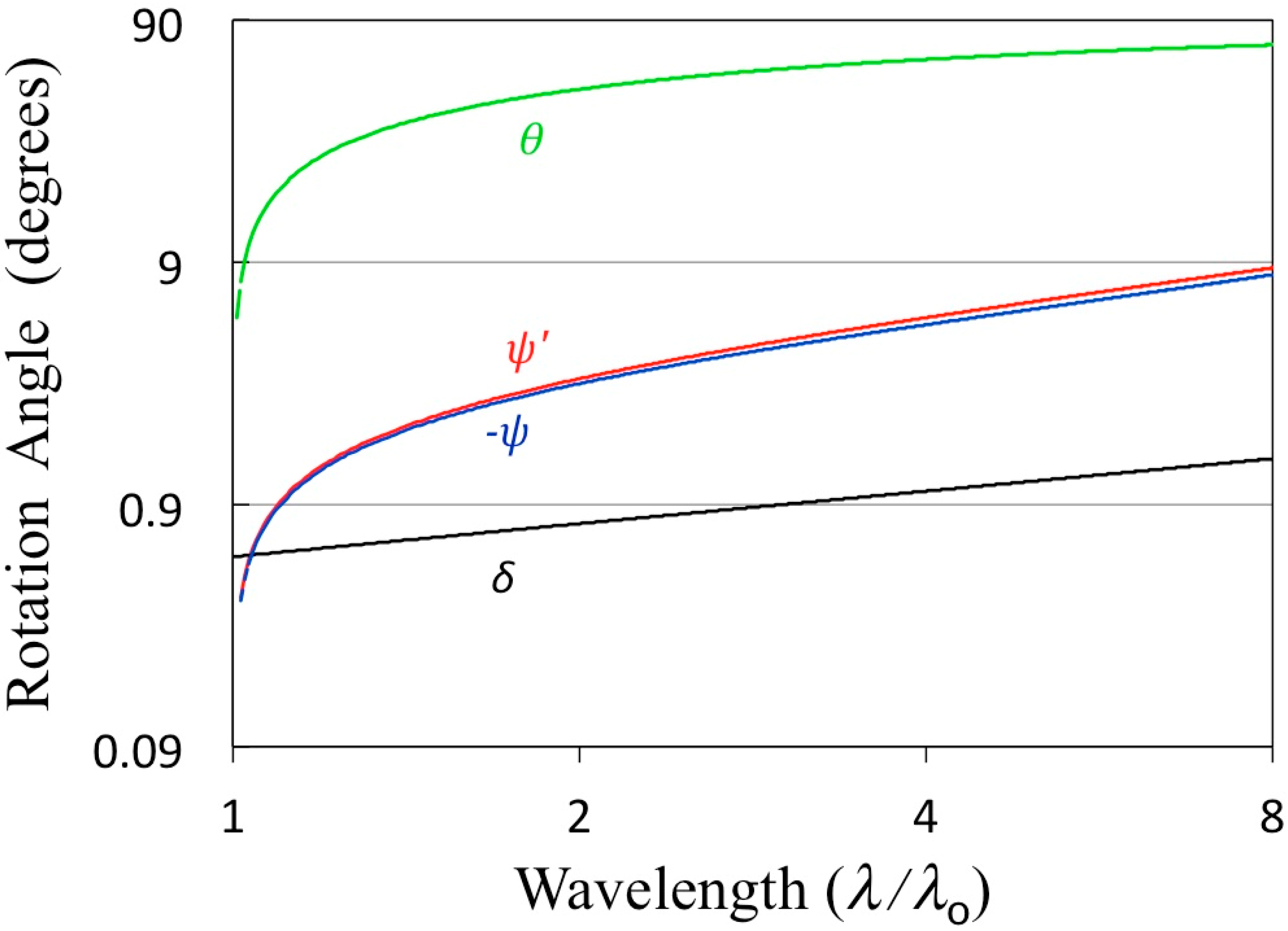
The required entrance and exit slit rotation angles, and , are plotted vs. scan wavelength in Figure 4. While these rotation values are comparable in magnitude, they are opposite in direction. This is due to the present treatment of the entrance slit as being an isotropic emitter (e.g., back-illuminated by a diffuse source), thus each point along the length of the slit has its own principal ray whose vertical coordinate reverses sign at the grating pole. However, if the entrance slit were illuminated by a distant horizontal (vertically-narrow) source, there would by a mapping between the z-values of points along the entrance slit and the sagittal pupil coordinate . This may be treated by a nonzero value of , as indicated in Section 3.2 and provided by the general expansion equations. The result would be no sign reversal of the required entrance slit rotation angle, opening the possibility for the entrance and exit slit rotations to be replaced by a third rotation of the grating (about its -axis), similar to the technique first employed in a SNR monochromator in 1993 as given in Section 4.2d of the cited thesis [15].
Figure 4.
The grating scan angles are (about the groove axis) and (about the surface normal axis). The entrance slit tilt angle () is slightly smaller in magnitude and opposite in sign (negated here for plotting convenience) than the exit slit tilt angle ().
The sequence of analytical calculations which determine the scan operating parameters are now specified:
(1) The grating first rotation angle , which sets and ;
(2) The grating second nominal rotation angle from Equation (58), using above ;
(3) Exact obtained numerically from Equation (57), with or without balance of spherical aberration (Equation (59));
(4) The dimensionless wavelength from Equation (10) or (12), using ;
(5) The exit slit tilt angle from Equation (56), using above ; and
(6) The entrance slit tilt angle from Equation (61), using above .
Using as specified above (and an object position ), the principal ray terms and aberrations are then determined from Equations (9,11) and (41–54), respectively. Transformation of the horizontal () and vertical () lateral positions to spectral resolution and exit slit height requires a final rotational transformation at the image plane, as given in Section 6.
5.5. Image Curvature
Spectral curvature along the image length is given by
which is the sum of three components (the paraxial position and two aberrations). The first term is the paraxial image curvature of a straight entrance slit, resulting in a deviation from a straight exit slit (albeit rotated in accordance with Equations (55), (56) or (60)) obtained by the rotational transformation of Equation (67) on the terms of the horizontal () and vertical () positions (Equations (11) and (9), respectively):
This component of the image curvature may be eliminated only by curving the entrance (not exit) slit. However, such correction is both difficult (due to its dependence on ) and unnecessary; for the example monochromator parameters, the uncorrected curvature at the ends of the 74 mm long image of the entrance slit is only microns at and decreases to microns at . This is confirmed (within 0.1 microns) by the numerical raytracings (1D profile of Figure 6i), revealing that the entrance slit length causes only a slight asymmetry and horizontal shift in the spectral line.
Horizontal curvature of the (vertical) astigmatism from a point source is given by (Equation (52)), often referred to as “sagittal coma” or “astigmatic coma”. This term, together with from Equation (45) determines the curvature in the spectral direction () using Equation (67):
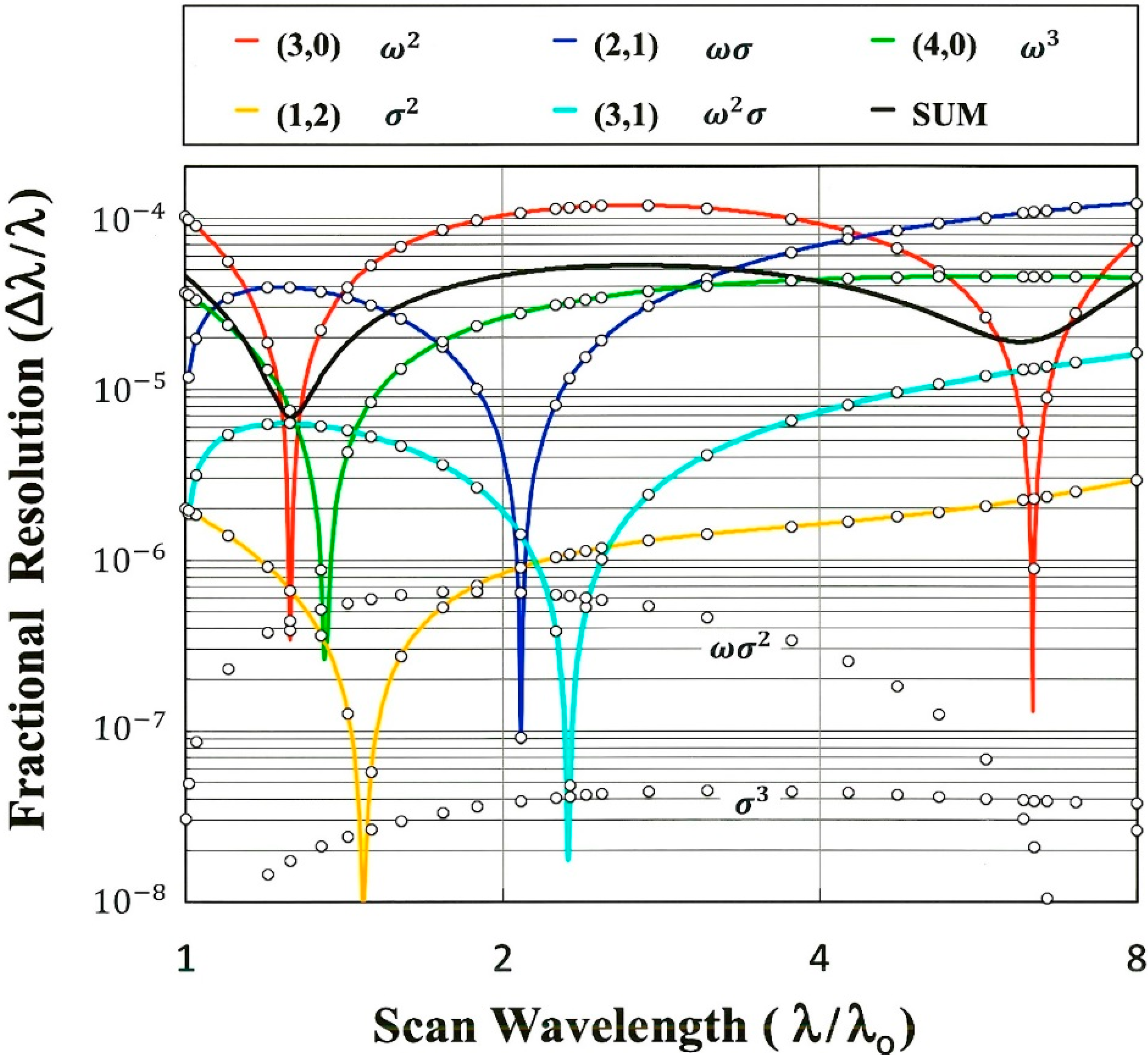
In spatial units, this resolution corresponds to 0.36 m at the minimum scan wavelength, zero at the (passive) correction wavelength () and 1.16 m at the maximum wavelength, confirmed by the numerical raytracings within 0.07 m. As given in Figure 5, these correspond to spectral resolutions () of 2 × 10⁻⁶, zero and 3 × 10⁻⁶, respectively.
It is noted that there are no (i,1) aberrations when 0, where the straight grooves are perpendicular to the meridional plane. In this case, the dominant mixed aberration is astigmatic coma (), for which the residual nonzero component of Equation (64) yields simply , independent of . This is the same result previously reported [8,15] for a plane grating in a converging (stigmatic) beam where While of importance and of historical significance in that original VLS application to fast XUV telescope beams (0.1), this aberration is negligible for most soft X-ray laboratory applications (e.g., 2 × 10⁻⁶ for 0.004). It is also noted that the passive correction point seen in Figure 5 may be obtained by zeroing the coefficient of the term in Equation (52), yielding 36°, though this aberration remains small across the scan range.
When expanded to include an off-plane () object point, the spectral aberration of sagittally-induced image tilt (), otherwise zero by proper rotation of the exit slit (Section 5.1), also has a small curvature component. However, because nonzero values of z are not included in the expansion of the aberration terms (i + j ) at present, the required horizontal and vertical component terms are not given in Equations (42) and (41), respectively.
5.6. The Horizontal Mixed Aberrations (2,1) and (3,1)
As shown in Figure 5, the dominant spectral aberration at long wavelengths is due to the (2,1) mixed term, which vanishes at one scan wavelength. A good approximation to this “passive correction” point may be obtained by zeroing the coefficient of the linear term in from Equation (47):
Simplifying this expression by treating and as small angles yields:
which occurs at 47.8° () for the example monochromator. However, this aberration is dominant at larger rotation angles, reaching a full-width comparable to that of the pure meridional (3,0) aberration at the long-wavelength end of the scan range (71.25°). As the magnitude of this mixed aberration scales with ωσ, it is highest at the corners of the solid aperture. An elliptically-shaped illumination would thereby halve the aberration with only a 22% intensity loss. However, for clarity the present analysis employs a simple rectangular aperture. The horizontal (2,1) ray aberration was also required to obtain the non-paraxial reference image position in the expansions of the (4,0) and (3,1) horizontal aberrations. As this is the dominant mixed aberration in the horizontal direction, the coefficients to degree were expanded so as to maintain accurate results even if increases (e.g., due to use of a higher graze angle).
As will be clear from the spectral resolution plot (Figure 5) and the raytrace diagram (Figure 6), the higher-degree (3,1) aberration causes only a small distortion to the above (2,1) aberration. Therefore, its laborious Fermat expansion (requiring nine lateral aberrations to compose the proper reference image, as listed in Table 2) was performed only for the linear component in and is given by Equation (54).
5.7. Minor Vertical Aberrations (1,2), (2,1), (3,1) and (2,2)
Given that the horizontal (1,2) aberration is very small, the vertical (1,2) aberration is surprisingly large (11 microns for the example design). This result would not be obtained from the standard light-path formulation, even given the aforementioned “astigmatism exception”. The aberration is correctly determined here by the inclusion of two additional non-paraxial reference points, namely , as listed in Table 2. Though not being of practical significance in itself for a (highly) astigmatic monochromator, the image plane rotation of Equation (67) transforms this vertical aberration into a non-negligible (1 micron) component of the (2,1) image width in the spectral direction. The vertical (1,2) aberration is also required as a non-paraxial reference for the correct expansion of the (dominant) horizontal (2,1) aberration.
Similarly, the vertical (2,1), (3,1) and (2,2) aberrations are of no importance in themselves, as they are comparatively negligible additions to the astigmatism term. However, their explicit expansions have been given in Section 4 to provide the comprehensive set of vertical reference image coordinates required for the expansion of the horizontal (3,0), (4,0) and (3,1) aberrations, respectively. The image plane rotation of Equations (67) and (68) also transforms the (2,1), (3,1) and (2,2) vertical aberrations into non-negligible components of the (3,0), (4,0) and (3,1) spectral aberrations.
6. Spectral Resolution
The spectral resolution equals the grating dispersion times the ray aberration normal to the slit length. The latter is determined by a rotational transformation of the image plane coordinates () to those of the -tilted image plane (). The power series is carried over to the coordinate by linearly combining the vertical and horizontal coefficients in accordance with:
Division by the linear dispersion per fractional wavelength yields the corresponding wavelength shift coefficients
where tan is given by Equation (56). The wavelength variation modulus () of each term over the full rectangular grating aperture () is its “extremum” (full width) aberration:
where if i is odd and j is even; otherwise ; and in which the full angular frontal apertures are sinα (meridionally) and (sagittally). Using Equations (67)–(69) with the constituent horizontal () and vertical () ray aberrations given by the light-path Equations (41)–(54), Figure 5 plots each of the nonzero spectral aberration terms . In the absence of spherical aberration balancing (Section 5.3), and are each zero relative to the rotated exit slit normal, as devised in Section 5.4 and Section 5.5. The and corrections for (3,0) and (4,0) specified in Section 2 are verified by Figure 5 to indeed minimize their peak magnitudes over the intended scan range of three octaves.
Figure 5.
Geometrical spectral aberrations of a soft X-ray single-element plane grating monochromator (SEPGM) at the Gaussian image plane. The grazing angular deviation is 6° and the incident aperture is 2 mrad horizontally × 4 mrad vertically. The meridional and sagittal aperture dependences of the individual terms are given in the legend, and plotted as extrema (peak-to-valley) over the full grating aperture. The colored curves result from rigorous expansion and Fermat differentiation of light-path functions, while the open circles are algebraic extractions from numerical raytracings at 29 wavelengths. Discrepancies between these two independent methods of analysis are negligible (~ 10−10 in ), being four orders of magnitude smaller than the physical diffraction width at a wavelength of 1 nm. The black curve is a conservative index of the net RMS geometrical resolution, summed from the individual terms (see the text).
An easily-calculable index of the net (measureable) spectral resolution is the root-mean-square (RMS) of the wavelength deviations (relative to that diffracted from the grating pole):
where ,, and where Equation (71) includes all terms up to a power-sum of 3, except for the insignificant terms of and . This RMS value is also plotted in Figure 5. The surface integral in Equation (70) corresponds to rays distributed uniformly on the grating surface, which differs somewhat from a uniform angular distribution originating at the object (source) point. It is also noted that the presence of asymmetrical aberrations, particularly the dominant (3,0) term, results in a nonzero mean value for the deviation. This offset causes Equation (71) to calculate somewhat larger values than a true “RMS width”, where the deviations would be calculated relative to the mean.
The first [bracketed sum] in Equation (71) contains a cross-product of the 20 (defocus) and 40 (spherical aberration) coefficients; by departing from the (abstract) condition of being “in-focus” (200), this product can be made negative and thus partially balance the positive and terms (as accomplished by the focus adjustment derived in Section 5.3). However, such (partial) balancing of these two different terms is aperture-dependent. Similarly, the second [bracketed sum] shows that combined coma may be made smaller than the sum of the positive meridionally-induced and positive sagittally-induced components. While exploited in normal-incidence optics (having a 3:1 ratio between these components), grazing angles result in the much larger (10:1) ratios evident in Figure 5, enabling little such coma balancing. The maximum value of sagittally-induced coma (1,2) is 2.9 × 10⁻⁶ at max71.25° (being only 1.5 times its in-plane value at 0) and is small compared to either the (25 times larger) meridionally-induced coma (3,0) or the (50 times larger) dominant aberration (2,1).
More generally, given a design optimized in resolution over a scan range of octaves, and given a ratio of between 10 and 100, meridional coma dominates the spectral aberration (provided the aperture aspect ratio ); fitting to several such sets of parameters yields the following approximate relation for the nominal resolving power () over the designed scan range:
This simple result shows a resolving power which scales quadratically with the graze angle and inversely with both the solid angle of acceptance and the spectral range. For the ultra-high resolution design plotted in Figure 5, 25 and 3, for which Equation (72) estimates (in agreement with the value of 29,000 obtained by averaging Equation (71) over the scan range). As specified in Section 5.3, optimization of the resolution for higher apertures (𝑒e.g., γ/ϕ ~ 8) requires some “least-confusion” defocusing to balance the dominant spherical aberration term. At yet higher apertures, several limitations would emerge: (1) spherical aberration would finally dominate and thus invalidate Equation (72); (2) more than a 50% line-space variation (Section 8.4) would be required; and (3) the large (12%) variation in graze angle in the meridional direction would compromise the average reflectivity.
In the direction along the slit length, the rotational transformation of the image plane yields
resulting in the following full-width aberrations in the direction parallel to the slit and relative to its center ():
7. Numerical Raytrace Simulations
Independent confirmation of the light-path equations derived in Section 2, Section 3, Section 4, Section 5 and Section 6 is obtained here by three-dimensional numerical raytraces, using the commercial code “BEAM4” developed by M. Lampton [16]. An angular deviation of 6° is chosen, as it provides a single-bounce gold reflectance of 50% at 1 nm in the soft X-ray. To display the optical aberrations, the raytraced source is a point at the entrance slit. However, if 5 micron wide slits are to contribute a dispersive component (Section 8.5) equal to the nominal optical resolving power of 25,000, the object distance must be r3000 mm. This scale converts the design parameters (listed in Section 2.6) to the following dimensional values:
| (Image distance) | 11,100 mm |
| (Line density at the pole) | 1000 mm−1 |
| (VLS ruling coefficients) | 20.955315252 mm−2 |
| 3−2.792863 × 10⁻⁴ mm−3 | |
| 41.906 × 10⁻⁷ mm-4 |
From Equation (4), one may easily determine the required accuracy for is thus (1000/25000)/(214 mm) 0.0002 mm−2 for 2. This translates to a groove positioning error of 0.0005 mm (1/2 groove width). This tolerance is 3 orders of magnitude less stringent than demonstrated (0.11 nm) by existing technologies in the fabrication of low scatter gratings [4,17]. To accept the 2 mrad () × 4 mrad () frontal aperture at every angular orientation () across the wavelength scan, the grating must have a physical aperture of 214 mm in diameter. At each value of , only the light-path equations given in Section 2, Section 3, Section 4 and Section 5 were used to determine the fixed (“cold”) inputs () for raytrace simulations run at 29 sample wavelengths across the three-octave scan range. No numerical optimization was performed by the raytrace routine (e.g., no “auto-focus” used).
7.1. Spot Diagrams
The right-hand panels of Figure 6 are the result of uniformly illuminating the grating rectangular pupil aperture with 10,000 randomly placed rays from the on-axis object point. Eight scan wavelengths were selected to highlight the different characteristic aberrations, and their convolutions, as listed in the caption. In these phase-space plots, horizontal sagittal coma (1,2) appears as a finite width at (visible only in Figure 6a), meridional coma (3,0) appears as a parabola (e.g., Figure 6a,d, with this also being a component aberration in Figure 6c,e,f,i), spherical aberration (4,0) causes a cubic (S-shaped) asymmetry between the – and regions (most evident in Figure 6a,f,g and i), the dominant mixed-term aberration of horizontal (2,1) appears as a “bow-tie” shape (in Figure 6b,c,e,f,g,h,i) and the minor mixed-term aberration of horizontal (3,1) causes the widths of the bow-tie to be different at the 2 ends (lopsided), as visible only in Figure 6g,h and i.
The bow-tie shaped aberration (2,1) is absent only for the in-plane orientation ( at which and at the passive correction point given by using Equation (66) for which . At those two wavelengths, the phase-space spot diagrams of Figure 6a,d show the classical curves resulting from the addition of the quadratic (coma) and cubic (spherical aberration) terms. Conversely, in Figure 6b these pure meridional aberrations are absent or small, resulting in the near-exclusive presence of the mixed aberration (2,1). It is also noted that Figure 6h confirms the least-confusion balancing (Section 5.3) of the defocus and spherical aberration terms given by Equation (59).
7.2. Line Profiles
The left-most panels in Figure 6 display the simulated (raytraced) spectra of the line doublet near three representative wavelengths within the scan range. The thick line segment shows the “RMS” value calculated by Equation (71). Due to the dominant aberration of coma (3,0) being more highly peaked than a normal distribution, the actual marginal optical resolution is much finer than the usual measure of a full-width-at-half-maximum2.355 RMS, except at the 2 coma-corrected wavelengths (and 6.58) where the marginal resolution is 1 RMS. Though Section 7.3 will reveal more quantitative detail for each aberration, it is evident in Figure 6 that the spectral resolution is comparable to or better than the 1/20,000 separating the two raytraced lines, thus confirming the net convolution of the light-path terms as plotted (black curve) in Figure 5.
Figure 6.
Numerical raytracings of an ultra-high resolution SEPGM, displayed in phase-space 2D spot diagrams ( vs. ) and 1D spectral profiles (intensity vs. ). The meridional pupil coordinate spans 140 mm at to 214 mm at 8, corresponding to 2 mrad in angular aperture. Wavelength increases to the top of each panel, in which the two wavelengths (shown here in green and red) are separated by 1 part in 20,000; their dispersed separation (9 microns at to 18 microns at 8) provides the dimensional scale for the image plane coordinate . (a) (0°): dominant coma (3,0), some spherical aberration (4,0) and slight sagittal coma (1,2); (b) 1.26: (3,0) canceled, dominant (2,1) and slight (4,0); (c) 1.43: (4,0) canceled, (1,2) nearly canceled, (2,1)–(3,0); (d) 2.08: (2,1) canceled, dominant (3,0); (e) 2.5: (3,1) canceled, dominant (3,0) near maximum, (2,1)–(4,0); (f) 5.2: dominant bow-tie (2,1), (3,0)–(4,0); (g) 6.58: (3,0) canceled, dominant (2,1), some (4,0), slight (3,1); (h) per 6(g), but with (2,0) adjusted to balance (4,0) for least-confusion; and (i) 7.99: (71.25°), (3,0)–(2,1)–(4,0), slight (3,1).
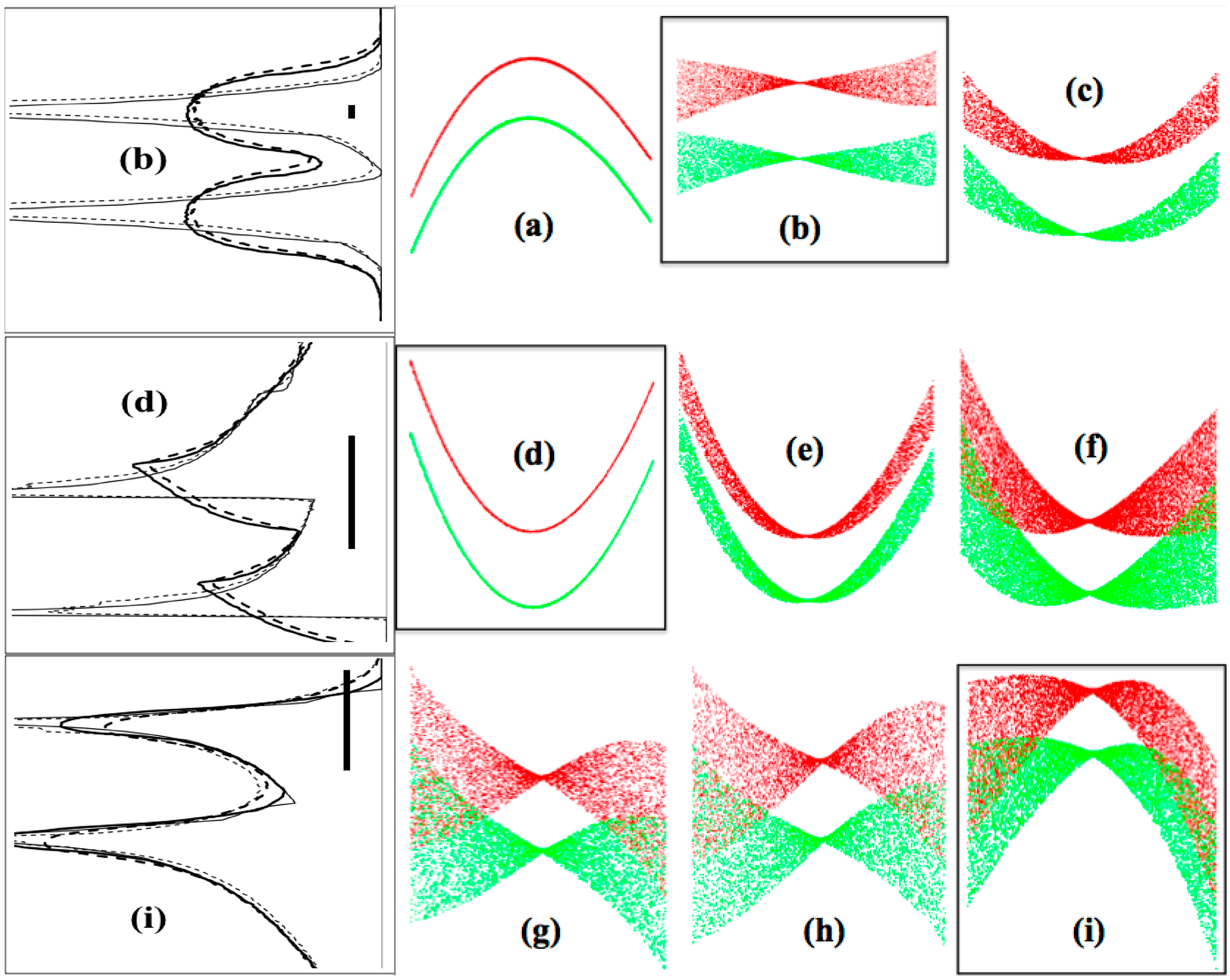
Four objects were used in the 1D simulations: a point (_____), as used for the 2D diagrams; a 3 horizontal width (____), a 20 mm long slit (------) and a 3 wide × 20 mm long slit (- - - -). The entrance slit was an isotropic source (equivalent to a passive slit backlit by a diffuse source) and tilted in accordance with Equation (61) for its image to coincide with the exit slit. The absence of any significant broadening in the line profiles obviates the need at present to include off-plane object () terms in the aberration expansions Equations (41)–(54) which were derived in Section 4 for a point source (). The 1D spectral profiles exhibit the following aberration ratios:
(b) ;
(d) ;
(i) .
The small longward shifts of the peak positions (compare the solid and dashed curves) for the 2 shorter wavelengths ((b) and (d)) is due to 1 micron image curvature of the straight entrance slit, as given by Equation (11). For the longest wavelength trace (i), the shift is seen to be in the opposite (shortward) direction and very small (0.2 microns), as predicted by Equation (63). “Pre-emptively” curving the entrance slit by a corresponding amount in the opposite sense (see Section 5.5) is found to eliminate such curvature and shift at the image plane (verified by a raytracing at ).
7.3. Power Series Extraction
Precise raytracings provide an alternate (and independent) method of determining the numerical value of the power series aberration terms derived from first principles in Section 3 and Section 4. Image positions (a “spot diagram”) from 21 pupil points are sufficient to extract all 20 component terms of power-sum (i + j − 1) 3, each free of contamination by any (other) term of power-sum 6. A numbered set of convenient grating pupil coordinate pairs used is:
where and denote the meridional and sagittal pupil half-widths, respectively. The difference (or sum) of two image plane positions, each relative to the principal ray, is written succinctly as (for example) , or (as another example) . It is also found that 13 pupil points (nos. 0 through 12) are sufficient to extract the same 20 terms, however with a small amount of contamination from (other) terms of power-sum 3.
The first two terms are simply the principal ray positions: ; . The remaining 18 are the extrema aberrations ( being the P-V variation in the lateral ray image positions over the rectangular grating aperture of and ). Each of these “extraction” Equations (75)–(92) are given in both 21-ray form and (after the “” sign) 13-ray form, followed by an identification of the lowest power contaminant term(s) for the latter. The indicated percentage level of contamination was determined, at the highest scanned wavelength (8) of the example monochromator, by comparing the results at two different values of the aperture in each direction, thus exposing its (distinct) power dependence, namely for and for .
The largest absolute contamination in the 13-ray extractions is % times the magnitude of the geometric aberration. As shown in Figure 5, the latter results in a maximum spectral aberration (at the longest wavelength) of 10−4, thus the 13-ray extraction is in error by only the negligible magnitude of 3 × 10⁻⁸. However, this contamination error was eliminated by use of the 21-ray extraction when calculating the deviations (given in Table 2) between the numerical (raytrace) extractions of Equations (75)–(88) and those calculated from first principles by the new (rigorous) light-path expansions of Equations (41)–(54). There are no adjustable parameters in either method, and thus no “fitting” of one to the other. The extremely small deviations shown in this table can therefore only be the result of both accurate light-path equations and accurate raytracings. For example, the raytracings illuminate the grating surface by the exact and centered rectangular aperture used in the analytical equations (), whereby (though the exact non-linear equation is used) is a strong function of as the grating is rotated. In addition, the formulations take equal care in the horizontal and vertical directions, as both spatial aberrations contribute to the spectral aberration. This is due both (directly) to the image tilt which includes the vertical aberration term in the rotational transformation of Equation (68), and (indirectly) to the need for inclusion of the vertical reference image position in Equation (37).
Equations (75)–(92) may be converted from extrema widths to power series coefficients by use of the transformations: . Using Equations (68)–(70), these terms were then converted to spectral aberrations and plotted in Figure 5 as the open circles at 29 raytraced wavelengths. Note that, as formulated in Section 5, the (tilted) spectral direction and the corresponding adjustment to the focusing condition cancels the effect of the first four aberrations (Equations (41)–(44) or Equations (75)–(78)), therefore Figure 5 shows no power terms of or , as they vanish to within the accuracy of the calculations. The last four extraction Equations (89)–(92) result in the 58 raytraced points for and each contributing less than 10−6. Due to these exceedingly small magnitudes (below the physical diffraction limit) and the large number of non-paraxial reference image coordinates required for their proper analytical expansion, the explicit equations for these have not been derived.
8. Practical Considerations and Enhancements
8.1. Vertical Deflection of the Principal Ray ()
The functional dependences of this off-plane deflection (Equation (9)) are most easily seen by applying the small-angle (grazing incidence) approximation to the grating Equation (10):
thus revealing that in Equation (9) scales with . At very shallow graze angles (½°) for use in the X-ray, the deflection is less than ¼ mrad even at the largest rotation angles considered here (71.25°), largely eliminating the need for vertical translation of the exit slit. However, grows to 5 mrad at 3° (soft X-rays) and to 60 mrad at 10° (extreme UV), being comparable to or exceeding the image length due to astigmatism.
This deflection may be compensated by the addition of a mirror which adjusts the vertical direction of the principal ray incident to the grating [15]. Absent such a mirror in the present “one-bounce” configuration, a translating iris may be used to provide off-center illumination of the grating, thereby maintaining a centered astigmatic image at the exit slit plane. In the case of the horizontal and vertical object conjugates being coincident (a point-like source), the iris center must align with an off-plane pupil coordinate determined by balancing Equations (9) and (41):
Unfortunately, this would not also cancel the off-plane direction of the diffracted rays, which would continue to cause an off-center illumination of any target significantly downstream of the exit slit.
The iris translation requires an incident beam of vertical angular extent (), being 4 mrad6 mrad for the example monochromator. In addition, the lateral aberrations which scale to powers of and higher will increase substantially as a result of the off-center grating illumination. Fortunately, these terms are generally insignificant, the largest one affecting the spectral resolution being horizontal (1,2) which is 2 orders of magnitude smaller than the dominant terms (see Figure 5).
8.2. Image Tilt
Using the grazing incidence approximation results in a simplified form of Equation (55):
revealing that the tilt is nearly linear with the graze angle. Consequently, rotations of the exit and entrance slits become less critical as the graze angle is reduced. For an X-ray version (½°), the maximum value of from Equation (61) is 1.3° and represents only 0.1 mm deviation at either end of a 10 mm long entrance slit. Such a small tilt may be accomplished by simpler and more accurate means than required for larger rotations.
8.3. Zero Order Overlap
The reflected zero order beam from a plane grating is unfocused, thus one must insure the exit slit does not lie within the specularly reflected diverging beam of undispersed light [10]. Such overlap is avoided if the meridional aperture 4, assuming 1; in the case of 1, substitute its reciprocal1/. To provide useable dispersion, is typically3/2 (or2/3), for which the aperture limitation becomes 0.8 . A tolerable (e.g., 40%) variation in graze angle across the optic independently constrains 0.4 , thereby placing the exit slit far into the shadow of the specular zero order light. The unfocused zero order is advantageous when using high peak-power sources, as it avoids a destructively intense focus of the integrated spectrum.
8.4. Required Variation in Spacing
Inserting Equation (15) for into Equation (6) determines the magnitude of this (dominant) linear component to the fractional variation of spacing across the ruled width:
For values of 0.04–0.12 (e.g., 2–6 mrad at 3°), 1.5 and 3–4, the required variation is 12–36%. Surprisingly, this is not significantly larger than the 10–29% variations required for a converging-beam geometry (−1) and is well within the factor 2 variations previously employed for 200 mm ruled width plane gratings in an astronomical spectrometer [15] (page 37). The sub-50% line density variation required of the present grating design is comparable to those successfully manufactured and provided in numerous (50) laboratory VLS spectrometer and monochromator systems designed and constructed by the author over the past 30 years, and thus are commercially available using existing fabrication methods.
8.5. Dispersive Resolution
Simple differentiation of the grating equation yields the contribution from (entrance; exit) slits of width to the fractional FWHM resolution of any single-grating monochromator as
where is the grating magnification. For the present typical values of 2 and 3.7, or their reciprocals, 1.27(. Thus, attainment of the average geometrical resolution shown in Figure 5 (4 × 10⁻⁵ or 10−4 nm) requires /r1.65 rad at 3° (e.g., 5 m, 3 m and a monochromator length of 14.1 m). The extremely low grating geometrical aberration of 10−5 nm near the first coma-corrected wavelength of 1.26 nm matches only exceedingly narrow (1 m) slits and a grating slope error tolerance of 0.05 rad; however the latter is attainable for plane surfaces.
8.6. Table-Top Version
At the other extreme from the ultra-high resolution performance displayed in Figure 5, a high-throughput version is parameterized by choosing 1/8, providing 10 times larger solid aperture. For the same graze angle (3°), the frontal aperture becomes 6.5 × 13 mrad and the resolving power is approximated by Equation (72) as 3000. Given this lower resolution, Equation (97) indicates a required physical length of only 2 m using the same slit widths (5 m). An extreme UV version (8°) of this “table-top” length monochromator would have a frontal aperture of 17.5 × 35 mrad and yield the same resolving power using slit widths of 15m.
8.7. X-Ray Version
For a given meridional aperture () and ruled width (r), the object distance r , resulting in from Equation (97). Therefore, at 1° (providing usable broadband reflectance to 5 keV in photon energy), an aperture of 2 mrad and a grating width of 214 mm requires r1 m (a monochromator length 4.7 m) and yields 2800. This figure matches the geometrical resolving power given by Equation (72).
Further reduction of the graze angle allows extension of the monochromator (same length and grating size) into the X-ray region ( nm). For example, ½° results in 1 mrad, 1400 and a scanning range of 0.125–1 nm (10–1.25 keV). It is noted that the first use of a pure (single rotation axis) SNR monochromator was at high energies, with a concave grating at 1° providing strong line spectra to 3 keV and first-order Bremsstrahlung continuum to its scan limit (4 keV) as shown in “Figure 4-4” on page 133 of the cited thesis [15]. The present design additionally benefits from recent advances in grating fabrication on smooth plane surfaces [4], and thus should extend efficient broadband grating spectroscopy to photon energies 5 keV.
8.8. Further Refinements and Additions
The detailed equations and raytracing results presented in this initial report demonstrate the fundamental spectral characteristics of the new geometry. Outlined here are a few possible variations to the basic single-element configuration, which may offer advantages dependent upon the graze angle, aperture, source size, performance priorities or desired versatility of the monochromator.
8.8.1. Linear Upstream Source
Inclusion of a nonzero value for (an object point whose z-coordinate has a linear dependence on ), corresponding to an entrance slit illuminated by a distant horizontal line. Such a case is allowed in the general light-path formulation (Section 3) and in Equations (32)–(34) of Section 4.1, but not included in the current explicit lateral aberration expansions (Section 4.2). Per Section 5.4, this longitudinal separation of the effective object plane in the vertical and horizontal directions may allow the required rotations of entrance and exit slits to be replaced by a (third-axis) rotation of the grating.
8.8.2. A Two-Element Monochromator with Astigmatism Control
A mirror may be added to focus (anastigmatically) or collimate in the vertical direction, the latter being previously used to maintain high spectral resolution without resort to a rotating slit in the case of a pure surface-normal rotation monochromator, as given in Section 4.3 of the cited thesis [15].
8.8.3. Choice of Magnification
In Section 2.6, the conjugate distance ratio () and the VLS coefficient N3 were chosen to eliminate coma (3,0) at two scan wavelengths. As the separation between these wavelengths vanishes, this optimization eliminates coma and its first derivative, resulting in a maximally-broad region nearly free of geometrical aberrations, centered on one wavelength. Alternatively, may be chosen independently (e.g. to provide a desired magnification = ), resulting in a narrower high-resolution region at the one scan wavelength where coma is eliminated by choice of N3.
8.8.4. Curved Grating Surface
A curvature of the grating surface, as already provided in the general light-path formulation (Section 3). Generalizing the graze-angle light-path approximations of Equations (14) and (15) to include a finite curvature radius (R) yields:
Combining the above two equations, the focusing condition () becomes:
For a given in-plane scan parameter , a radius which is positive (concave), but larger in magnitude than that required for a constant line-space () grating to focus, requires an increase in , while a negative (convex) radius requires a decrease in . From the approximate grating Equation (93), these changes in result in a more extended scan range () for a concave grating and a (slightly) reduced scan range for a convex grating. An interesting case is when the radius is positive and smaller in magnitude than the constant line-space self-focusing radius, the latter of which completes the equations of this paper on a classical note:
In the case of , the surface curvature provides too strong of a focusing power, requiring the VLS to weaken this by a change in sign of . The result is that the required value of decreases sharply (for a given ). For the parameters of the example ultra-high resolution monochromator, choosing is numerically found to minimize ; at 2.73, rather than the plane grating requirement of . However, this reduces the maximum scan wavelength from 8 to 3.2 . Nonetheless, the advantage of this curved grating design is that this is still significantly smaller than the value of 58° required by the plane grating design at the same wavelength. Thus, for this (more limited) scan range, the curved grating results in a significant decrease (factor 2) in the required slit tilts and 30% decrease in the vertical image deflection.
Equation (98) with provides three free parameters (), potentially enabling the cancelation of coma () at an additional (third) scan wavelength or the cancelation of spherical aberration () at an additional (second) scan wavelength.
8.8.5. Extended-Range Configurations
Dimensionless Equations (14)–(16) reveal that the horizontal focusing (first, second and third degree) and the VLS ruling parameters () are nearly independent of graze angles. Therefore, the same physical grating, object and image distances provide nearly the same imaging performance at any small angular deviation 2. As with other self-focusing plane grating geometries, this requires the in-plane (initial) value of the scan parameter () to be unchanged, which is arranged by simply re-adjusting the initial grating normal angle ] per Figure 1.
For example several stationary exit slits at various horizontal locations could provide different values of scaling with per Equation (93). Though a linear scaling of wavelength with graze angle would maintain the blaze of phase-diffraction grooves and provide roughly equal reflection coefficients from a gold surface for 10 nm, the scaling is near optimal for obtaining reasonable (0.2–0.9) reflectances over the entire 10-octave region (0.125–120 nm) where grazing incidence is of advantage. This enables construction of an ultra-wide range monochromator employing multiple (5) exit slits, each providing a band spanning three octaves in wavelength:
- 21° (X-ray band, 0.0625–0.5 nm); reflectance 10% below 0.125 nm (60°)
- 22° (Deep SXR band, 0.25–2 nm)
- 24° (SXR band, 1–8 nm)
- 28° (XUV band, 4–32 nm)
- 216° (EUV/FUV band, 16–128 nm)
A single amplitude reflection grating could provide a constant relative diffraction efficiency and good suppression of higher spectral orders (), or multiple blazed gratings could be interchanged to provide a higher (peak) efficiency in each band. The slit rotations would scale with (per Equations (55) or (95)), as would the dispersive limit to the resolving power (per Equation (97)). If used at high spectral resolution, then the exact (-dependent) focusing condition of Equation (57) would be enforced by adjustments to the angle for each band.
As an alternative to the use of multiple slits, a conventional plane pick-off mirror (rotating-translating or rotating off-axis) could be inserted into the diffracted beam to direct each angular deviation along the same exit axis. Though such a plane mirror does not alter the basic focusing characteristics of the optical system, while further suppressing the higher spectral orders by preferential absorption, such a configuration requires at least two reflections (reducing its efficiency).
8.8.6. A Two-Element Time-Compensated Monochromator
A tandem grating configuration can substantially cancel the groove-to-groove phase differences defining wavefront division for an individual grating, thereby providing a common path-length within the aperture of the emerging beam. The new rotation scheme enables the construction of such a monochromator using only two plane grating reflections, eliminating the need for the additional two concave mirrors employed with current state-of-the-art time-compensated monochromators [18].
9. Conclusions
At fixed conjugate distances and horizontal deviation angle (2), self-focused grazing-incidence gratings defocus rapidly upon (groove-axis) in-plane rotation. This is due either to the use of a curved (concave) surface or to the change in (ratio of diffracted graze angle to incident graze angle) which determines the focusing condition of plane gratings. However, if varied line-spacing (VLS) provides the focusing power rather than surface curvature, strong defocusing also results from a surface-normal (off-plane) rotation, which can therefore be used to cancel that from the in-plane rotation. These concerted rotations also reinforce the change in wavelength, extending the scan range beyond that available from a single rotation. A new scanning geometry and class of monochromator has thereby been invented which requires only one plane surface, representing a terminal point in the progression of grazing incidence monochromator designs towards fewer and simpler surfaces.
Small-angle approximations to the light-path equations for a plane grating provide a clear understanding and classification of the essential spectral aberration characteristics for different optical geometries. This simplifies the equations, clearly revealing the imaging properties which are (nearly) independent of the graze angle. A more rigorous analysis of the imaging properties exhibited by the new monochromator geometry has precipitated the (incidental) introduction of two mathematical tools of more general applicability in aberration analysis; being an expansion formulation based on non-paraxial reference points and an extraction of aberration series coefficients from raytrace simulations:
(1) The small spectral aberrations and dominance of off-plane terms in the present monochromator geometry has unveiled a flaw in standard light-path formulations. A mathematically rigorous general light-path expansion theory has been introduced, which systematically employs reference wavefronts centered on non-paraxial image points. This procedure, while more complex than the standard approach, correctly isolates each power-term of the path-length series. Interestingly, comparison of the two formulations reveals that the standard approach does not in general provide the correct expansion (or consequently the total aberration), being inexact even in the simple case of a spherical mirror.
(2) An accurate method has been introduced for extracting the individual geometrical terms from the image positions of a small number (13–21) of numerically traced rays. For 14 of the 18 lateral aberrations of power-sum , a detailed comparison between these extractions and the analytical equations (derived from the new light-path formulation) shows essentially exact (10−11 radians) agreement, being several orders of magnitude finer than the physical diffraction width. This precision suggests that such extractions may be used in the future to infer (rather than derive) the Fermat equations, by composing them from an algebraic template of geometric parameters fit to the raytrace extractions. However, such numerical fitting has not been used in the present work, rather all equations have been derived from first principles.
Initial use of a meridional-only approach (based on the standard theory and the graze-angle-invariant approximation) and final use of the rigorously-developed (non-paraxial image reference) light-path formulation, have provided equations for various focusing conditions (horizontal, spectral and least-confusion spectral) by correlation of the two grating rotations. The theoretical analysis has also derived the required exit slit tilt () and entrance slit tilt () as functions of the scan parameters, the VLS ruling coefficients () for self-focusing and correction of the higher-degree meridional aberrations, an optimized value for the mount parameter () which provides cancelation of the higher-order (3,0) meridional aberration at two chosen wavelengths and explicit expansion equations of ultra-high accuracy for the 14 leading lateral aberration terms.
The spectral resolving power may be approximated by over a scan range of octaves for a collection aperture of (meridional) × (sagittal) radians. This large product of spectral resolution, solid aperture and scan range is due to the high level of aberration-correction provided by this geometry (particularly the cancelation of coma at 2 wavelengths) combined with the multiplicative change in wavelength provided by the two rotation motions. Such a high figure of merit may be parameterized between these 3 components (resolution, aperture and scan range) as desired, with examples given for an ultra-high resolution (25,000) soft X-ray “beamline” version (14 m length), a high collection aperture “table-top” version (2 m length) and an X-ray version (½°).
Supplementary Files
Supplementary File 1Conflicts of Interest
The authors declare no conflict of interest.
Appendix A. A Simple Illustration
Figure A1 compares the two light-path calculations (“standard” and “rigorous”) of spherical aberration (4,0) vs. magnification for the simplest and most common focusing optic, namely a spherically concave mirror.
Figure A1.
Calculated aberrations of a spherical concave mirror at the Gaussian focus. The second-degree (“coma”) lateral ray aberration is correctly calculated by either the standard or the rigorous light-path formulations; the open circles are independent extractions of this term from numerical ray tracings. Light-path calculations of the third-degree (“spherical aberration”) lateral ray aberration are compared for the standard (dashed), semi-standard (dot-dashed) and rigorous (solid) formulations, with the open circles being independent extractions of this term from numerical raytracings. In this example, the object distance is 1000 mm, the graze angle is 10° and the acceptance aperture is 20 mrad.
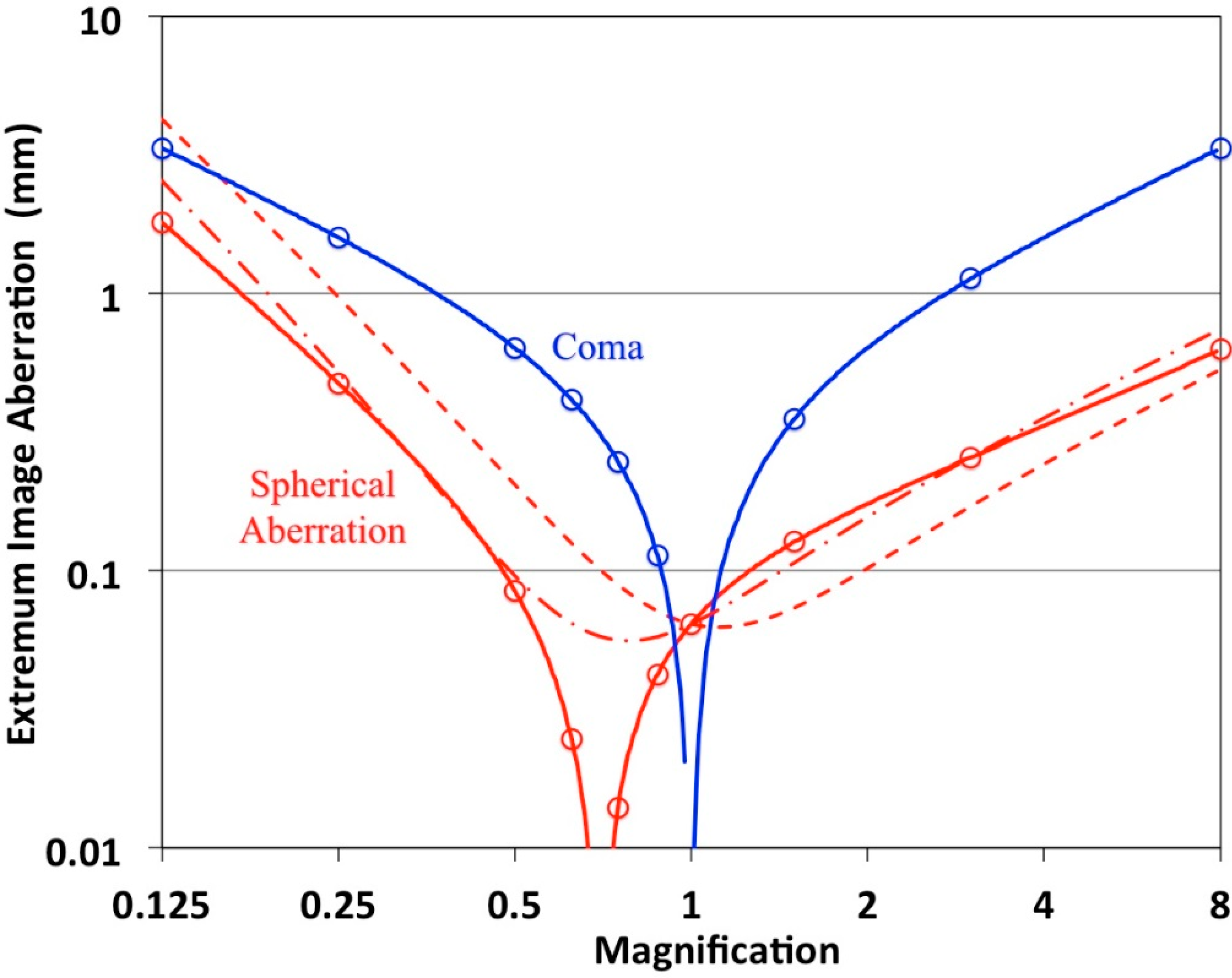
The first-degree lateral aberration (“defocusing”) vanishes for a mirror curvature , where is the graze angle. Given this constraint, there is no aberration (non-paraxial position) to include as the reference image for calculating the next higher aberration (second-degree “coma”), so the latter result is the same as given by the standard formulation:
Given the same in-focus constraint, the expansion term for spherical aberration simplifies to:
where,
and,
in the standard formulation (paraxial image reference).
However, to formulate rigorously, one must use Equations (19), (22), (24), (26) and (29) with (on-axis point source), (mirror), 0 (no sagittal rays), S (spherical surface) and the inclusion therein of the existing lateral ray aberration from Equation (A1) as a non-paraxial image reference point . The resulting value of is unchanged compared to the standard result, due to only the first term of Equation (A2) surviving when (normal incidence), and in this case there is no aberration and thus only the standard paraxial image point. However, the rigorous formulation yields a different value for . In addition to using as the (non-paraxial) reference image point and employing the Fermat differential of Equation (26), the grating curvature term of Equation (29) is significant, adding to the value of . The result is:
which equals Equation (A4) of the standard expansion only at 1, where vanishes for all . In the more general case (1 and , is nonzero and Equation (A5) differs from Equation (A4). As plotted in Figure A1, this discrepancy is clear and seen to be independently confirmed by the overlayed data points from numerical raytrace extractions. Due to the high angular aperture (20 mrad), the “uncontaminated” (21-ray) version of Equation (85), employing seven rays across the pupil meridian at each magnification, was used to insure an accurate extraction of . This results in essentially exact agreement (0.000005 mm at all but the two lowest magnification points) with the rigorous expansion.
Salient specific results of potential interest for optical designers are apparent from Figure A1: (1) The standard formulation under-calculates spherical aberration for magnifications1, while it significantly over-calculates this term for magnifications1; (2) Spherical aberration vanishes at 0.7, which for grazing angles is very near the root of the cubic equation given by 0. Including the term, the exact value of this “sweet spot” is at 0.697, 0.697, 0.704, 0.718 and 0.740 at respective graze angles of 3°, 10°, 45°, 60° and 70°, the latter two representing a “near-normal incidence” condition; and (3) The standard formulation (dashed curve) incorrectly identifies (“spherical aberration”) as comparable to (“coma”) at low magnifications. Figure A1 shows that the extremum (P-V) of remains significantly smaller than that of even at the very low magnification of0.125. Figure A1 also shows the result of spherical aberration calculations using a semi-standard formulation (dashed-dot curve), whereby the trailing term of Equation (29) is included, but the paraxial reference image is (erroneously) maintained. The equation for then becomes .
Compared to the classic horizontal focusing mirror example given above, the errors inherent in the standard light-path formulation are more significant for a surface-normal rotated diffraction grating, and increase further in the presence of varied line-spacing. Firstly, such a geometry gives rise to numerous mixed terms, especially large being those of (i,1), and thus a proliferating 2D power matrix of non-paraxial reference image points. Secondly, the image rotation (1,1) terms cause a transfer of (otherwise insignificant) vertical aberrations into rotated slit-normal (spectral) components. Thirdly, the inclusion of vertical aberrations as image reference coordinates in the rigorous formulation of horizontal light-path terms (and vice versa) requires that even non-dominant aberrations be initially calculated accurately to avoid significant errors in the subsequently expanded higher-degree terms. For the above reasons, the standard formulation does not provide an accurate prediction of the aberrations for the new design, or for other off-plane diffraction mountings in non-stigmatic geometries. As specific examples, refer to the discussion in Section 4 and the Table 2 entries for the horizontal aberrations and , which are dominant terms of the new optical design and thus require accurate formulation.
Appendix B. A Rigorous Algebraic Expansion in Detail: The (2,1) Horizontal Aberration
From Equation (29):
where, from Equation (5)
from Equation (38):
and,
from Equation (35) in which, from Equation (37):
where the reference image terms ( and ) and their products are derived from Equation (23) as:
Using the substitution
and expanding to include all the terms in , which then become terms in :
Grouping like power terms together:
where,
From Equation (B4):
where,
yielding Equation (47) as it appears in the main text:
Appendix C. Cancelation of Vertical Deflection: 3-Axis Grating Rotation
Additionally rotate the grating about its third axis, namely that defined in Figure 1 and Figure 2b by the meridional coordinate ω. From Equation (9) it is approximated that such rotation by an angle
will correct for the principal ray vertical deflection (z′01). This new scan angle is plotted in Figure C1 for the ultra-high resolution monochromator parameterized in the paper. Also plotted are the scan angles required of the exit slit (𝜓′) and entrance slit (𝜓) re-oriented by subtracting Ω from Equations (55) and (61), respectively. Using the longest scan wavelength (λmax/λo = 7.9945343) as the most sensitive test, these approximations yield Ω ≃ 4.1488°, 𝜓 ≃ −12.158° and 𝜓′ ≃ 4.3898°.
Figure C1.
Scan angles of the grating (δ, , ) and slits (, ) for a 3-axis grating rotation where = 0. Compare to the 2-axis grating rotation (Figure 4) where ≠ 0.
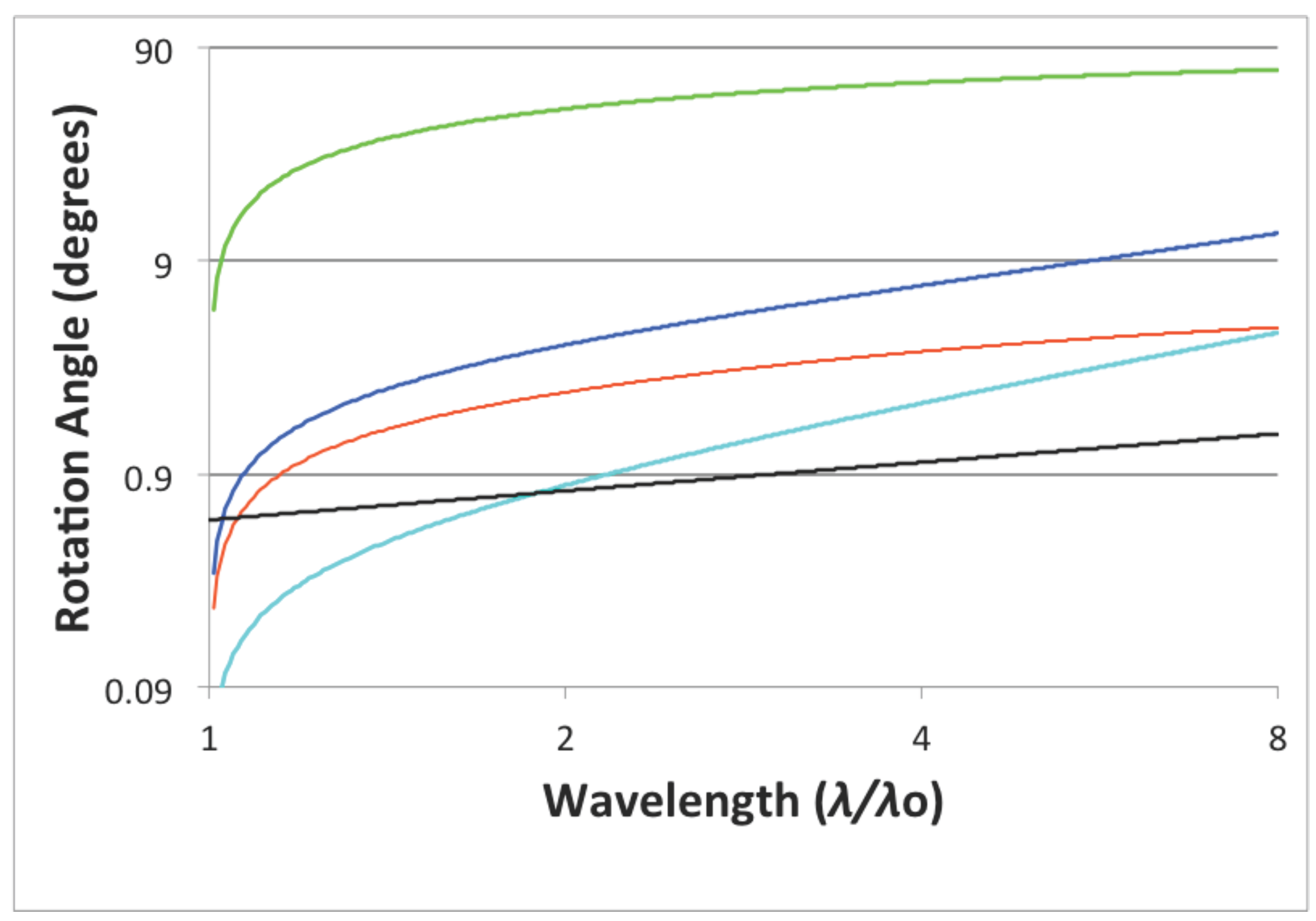
Numerical raytracings have also been performed to independently, and more precisely, determine the optimum 3-axis grating orientation at the scanned wavelength. This was conveniently provided by the “auto-adjust” routine of BEAM4 [16] in a least-squares minimization of the spectral image width. At λmax this numerical procedure yielded δ = 1.3951844°, θ = 71.40978°, Ω = 4.1525°, 𝜓 = −12.158° and 𝜓′ = 4.4083°. For reference, the scan angles for the 2-axis grating rotation (Ω = 0) are δ = 1.3915105°, θ = 71.24507°, 𝜓 = −8.009° and 𝜓′ = +8.5386°, resulting in z′01 = −84.03 mm. In the 3-axis scan proposed here, the fixed trajectory of the diffracted principal ray simplifies the exit slit rotation to be that about a stationary axis (located at = 0, = 0). Full-aperture numerical raytracings also reveal spot diagrams and spectral resolution of the undeflected images (z′01 = 0) which are nearly identical to those shown in Figure 6 (for which the vertical deflection at λmax is ~ 84 mm). Thus, the aberration correction is maintained.
From a mechanical engineering standpoint, upgrading from a 2-axis to a 3-axis goniometer for precise rotation of the grating is more compact and convenient than providing vertical translations of the exit slit rotation axis and the downstream target. Note that both these translations would need to be accurately coordinated with the basic 2-axis grating rotation. Furthermore, in the case of complex or large target stations, it is often impractical to even consider such translation.
The proposed grating rotation about its meridional axis will also remove the vertical deflection inherent in the (simpler) pure surface normal rotation monochromator [2]. Given rotation about both its surface normal axis and its meridional axis, a constant line-space concave grating can focus on its Rowland circle and its principal ray remains fixed in the horizontal and vertical directions.
References
- Hettrick, M.C. In-focus monochromator: Theory and experiment of a new grazing incidence mounting. Appl. Opt. 1990, 29, 4531–4535. [Google Scholar] [CrossRef] [PubMed]
- Hettrick, M.C. Surface normal rotation: A new technique for grazing incidence monochromators. Appl. Opt. 1992, 31, 7174–7178. [Google Scholar] [CrossRef] [PubMed]
- Hettrick, M.C. Grating Monochromators and Spectrometers Based on Surface Normal Rotation. U.S. Patent 5,274,435, 1993. [Google Scholar]
- Greiner, C.M.; Iazikov, D.; Mossberg, T.W. Diffraction-limited performance of flat-substrate reflective imaging gratings patterned by DUV photolithography. Opt. Express 2006, 14, 11952–11957. [Google Scholar] [CrossRef] [PubMed][Green Version]
- Hunter, W.R.; Williams, R.T.; Rife, J.C.; Kirkland, J.P.; Kabler, M.N. A Grating/Crystal Monochromator for the Spectral Range 5 eV to 5 keV. Nucl. Instr. Meth. Phys. Res. 1982, 195, 141–153. [Google Scholar] [CrossRef]
- Petersen, H. The Plane Grating and Elliptical Mirror: A New Optical Configuration for Monochromators. Opt. Commun. 1982, 40, 402–406. [Google Scholar] [CrossRef]
- Lu, L.; Cocco, D.; Jark, W. Simple plane grating monochromator for synchrotron radiation. Nucl. Instr. Meth. Phys. Res. A 1994, 339, 604–609. [Google Scholar]
- Hettrick, M.C.; Bowyer, S. Varied line-space gratings: new designs for use in grazing incidence spectrometers. Appl. Opt. 1983, 22, 3921–3924. [Google Scholar] [CrossRef] [PubMed]
- Hettrick, M.C.; Underwood, J.H.; Batson, P.J.; Eckart, M.J. Resolving Power of 35,000 (5 mÅ) in the extreme ultraviolet employing a grazing incidence spectrometer. Appl. Opt. 1988, 27, 200–202. [Google Scholar] [CrossRef] [PubMed]
- Itou, M.; Harada, T.; Kita, T. Soft x-ray monochromator with a varied-space plane grating for synchrotron radiation: design and evaluation. Appl. Opt. 1989, 28, 146–153. [Google Scholar]
- Namioka, T. Theory of the Concave Grating I. J. Opt. Soc. Am. 1959, 49, 449–460. [Google Scholar] [CrossRef]
- Beutler, H.G. The Theory of the Concave Grating. J. Opt. Soc. Am. 1945, 35, 311–350. [Google Scholar] [CrossRef]
- Howells, M.R. X-ray Data Booklet, 3rd ed.2009; Section 4.3.B; pp. 18–23. Available online: http://xdb.lbl.gov/xdb-new.pdf (accessed 16 December 2015). [Google Scholar]
- Born, M.; Wolf, E. Principles of Optics, 6th ed.; Pergamon Press Ltd.: Oxford, England, 1980; p. 207. [Google Scholar]
- Hettrick, M.C. Optical Design and Experimental Development of Grazing Incidence Fixed Slit Spectrometers for High Resolution Plasma Diagnostics. Ph.D. Thesis, The Graduate University for Advanced Studies, Department of Fusion Science, Gifu, Japan, 1996. Available online: http://www.hettrickscientific.com/pdf/thesis/Hettrick%20phd%20thesis.pdf (accessed on 3 March 2016). [Google Scholar]
- Stellar Software. BEAM FOUR: Optical Ray Tracer, Java v. 154. Available online: http://www.stellarsoftware.com (accessed on 22 October 2015).
- Harada, T.; Kita, T. Mechanically ruled aberration-corrected concave gratings. Appl. Opt. 1980, 19, 3987–3993. [Google Scholar] [CrossRef] [PubMed]
- Frassetto, F.; Miotti, P.; Poletto, L. Grating Configurations for the Spectral Selection of Coherent Ultrashort Pulses in the Extreme-Ultraviolet. Photonics 2014, 1, 442–454. [Google Scholar] [CrossRef]
© 2016 by the author; licensee MDPI, Basel, Switzerland. This article is an open access article distributed under the terms and conditions of the Creative Commons by Attribution (CC-BY) license (http://creativecommons.org/licenses/by/4.0/).