1. Introduction
Maxwell’s equations are a set of partial differential equations governing the electromagnetic (EM) waves [
1]. Solution to the Maxwell’s equations is very important for studying many physical phenomena. Among many methods for solving Maxwell’s equations, the Finite-Difference Time-Domain (FDTD) method is one of the most popular numerical approaches [
2]. Here, we numerically investigate the solution of Maxwell’s equations in nonlinear media and its application to nonlinear optics.
Recently, experiments have shown that strong nonlinear response such as the second-harmonic wave can be generated from Split-Ring Resonator (SRR) [
3,
4,
5,
6]. The SRR consists of array of U-shaped metallic gold nanoparticles. Under the excitation of an external electromagnetic wave, strong nonlinear optical wave is generated. A classical theory based on the cold plasma Maxwell’s equations are developed in [
6,
7,
8] to study the nonlinear optical response for this structure. In [
6,
7], perturbation expansion of nonlinearities is used in order to solve the cold plasma-Maxwell’s equations. In [
8], a nonlinear Drude model is developed and solved by a time-splitting finite difference method. In [
9,
10], full fluid equations (Euler’s equations) are coupled to the Maxwell’s equations and is solved by perturbation expansion of nonlinearities. In [
11], the discontinuous Galerkin time domain method and the hydrodynamic Maxwell-plasma model are applied to simulate the linear and nonlinear optical response from SRR arrays.
In this paper, we numerically study the solution of the hydrodynamic electron fluid Maxwell equations by solving the electron density and momentum equations using an explicit finite difference hyperbolic PDE solver together with the FDTD method for the Maxwell’s equations. This work is the extension of the previous work in [
7,
8] to electron fluid equations containing both electron density equation and the electron current equations with the electron pressure term included. We apply our model to simulate the nonlinear optical responses such as second-harmonic generation (SHG) from metallic nanoparticles and the numerical results yield good agreement with the experimental results published in [
3,
4,
5].
2. Numerical Model of Hydrodynamic Electron Fluid Maxwell Equations
The hydrodynamic electron fluid Maxwell equations consists of the Maxwell’s equations
and the hydrodynamic electron fluid equations
where
and
represent vacuum permittivity and vacuum permeability, respectively.
,
,
and
are the electron density, velocity, electron mass and electron charge, respectively. The damping factor
γ is added to describe the current decay due to Coulomb scattering. Equation (2) is the continuity equation and Equation (3) is the equation of motion (momentum conservation).
p is the quantum pressure given by Thomas-Fermi theory,
where
From Equations (2) and (3) we get
Let
, and current density
, which can be written as nonlinear hyperbolic system in conservation form
where ⊗ is the tensor product.
For convenience, we rewrite the above system into the following conservation form
where
In this paper, we apply the standard space and time staggered grid based FDTD method to solve the Maxwell’s Equation (1) and a non-staggered grid based central difference method to solve the hyperbolic Equation (7).
The FDTD Method is based on the space-time staggered Cartesian grid. The three components of the electric fields and the three components of the magnetic fields are defined at different positions in space and time. The electric fields are defined at the time step of
τ; the magnetic fields are defined at the time step of
. In a computational cell
, three components of electric fields,
,
, and
, are defined at the locations of
,
, and
, respectively; three components of magnetic fields,
,
, and
, are defined at the locations of
,
, and
, respectively. Since the current density
J is defined at the same location as
E in space and at the same location as
H in time, our numerical method requires all components of J to be interpolated at cell corners. Hence, we define new variables
at cell corners such that
We use the central difference method for solving the Equation (7), and its discretization form is given as
In the update Equation (11),
When getting the value of
and
, we average them to get the value of
,
, and
as follows:
Therefore, we have
which has filtering effect. Our numerical simulations show that the above central difference method provides stable solution.
3. Numerical Simulation of SHG from SRR
In this section, we simulate the optical second-harmonic generation (SHG) from metallic nanoparticles numerically using the numerical solver presented in the previous section. The simulation results are compared with optical experimental results shown in the paper [
3,
4,
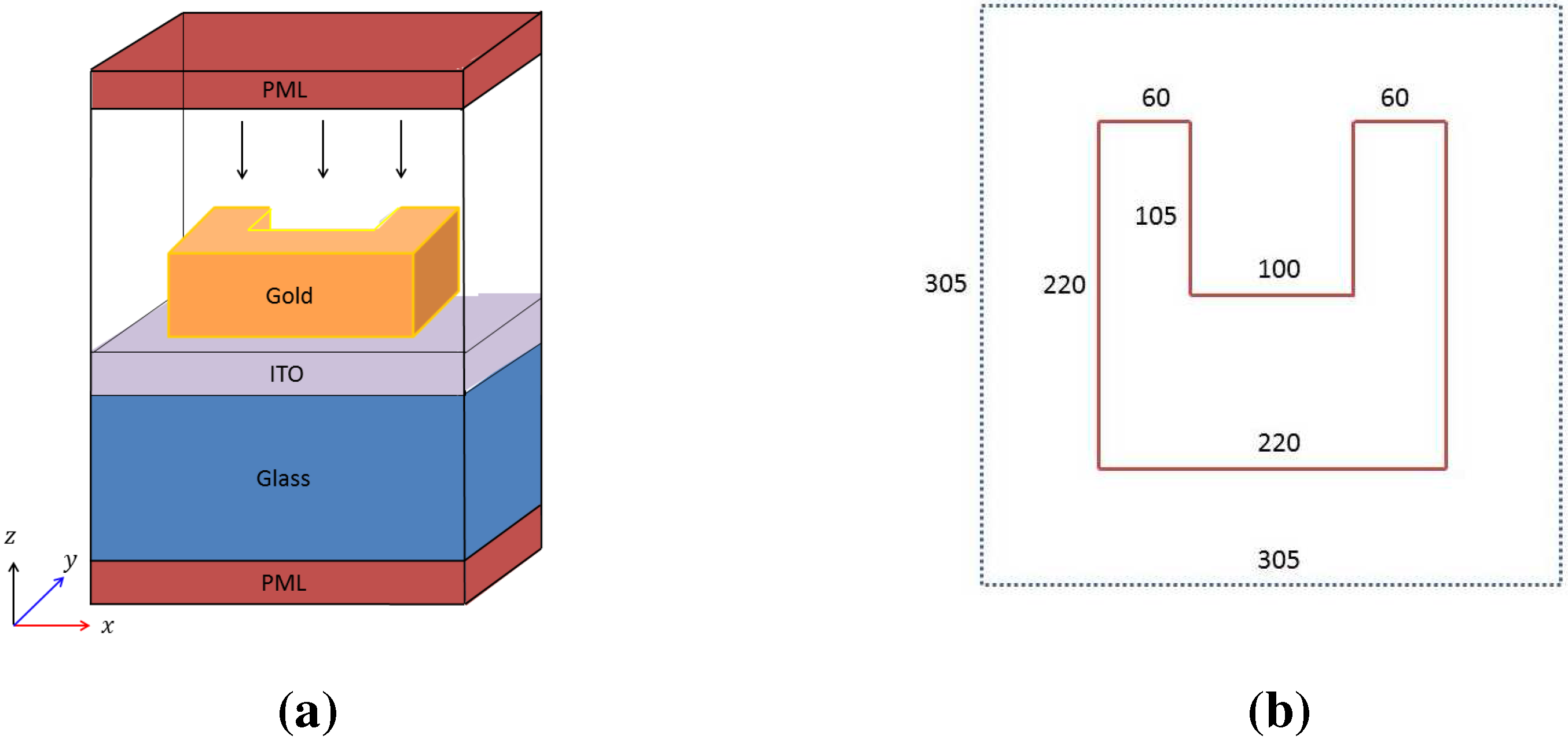
5]. The simulation setup is shown in
Figure 1a. The red arrow represents the direction of incident pulse; the blue arrow represents the direction of second harmonic waves. A three-dimensional gold nanoparticle is placed in the middle of the computational domain with periodic boundary conditions in both
x and
y directions. Perfectly Matched Layers boundary condition is applied in
z direction. The gold nanoparticle is U-shaped with plasma frequency
and phenomenological damping factor
, and thickness of
. The
cross section of the U-shaped gold nanostructure is shown in
Figure 1b. ITO (
and
thick) and glass (
below ITO to the bottom) substrates are placed beneath the particle. The rest of the computational domain is vacuum.
The incident Gaussian pulse with carrier wavelength
is excited in
x direction and propagates along
z-axis. Its profile is given by
where
. The strength of the incident pulse is
. The energy conversion efficiency of the SHG is defined by
where
represents the incident pulse,
is the second-harmonic signal,
is the dielectric permittivity of the substrate.
Figure 1.
(a) The computational domain for optical pulse propagation through three dimensional gold nanostructures; (b) cross-section of the U-shaped gold nanostructure with the unit of .
Figure 1.
(a) The computational domain for optical pulse propagation through three dimensional gold nanostructures; (b) cross-section of the U-shaped gold nanostructure with the unit of .
In our numerical simulations, we choose uniform grids given by and according to the Courant-Friedrichs-Lewy condition number of 0.5.
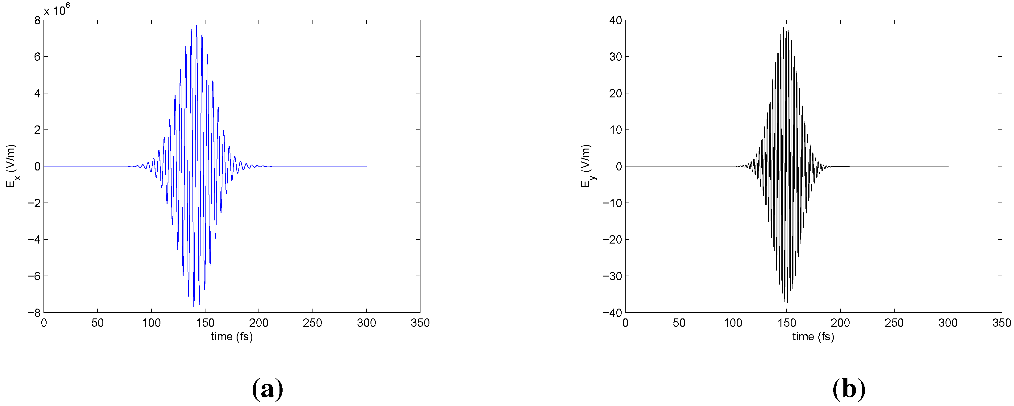
Figure 2a shows the time history of linear (
) and nonlinear second harmonic (
) waves for U-shaped metallic particles illuminated by
x-polarized incident light. In
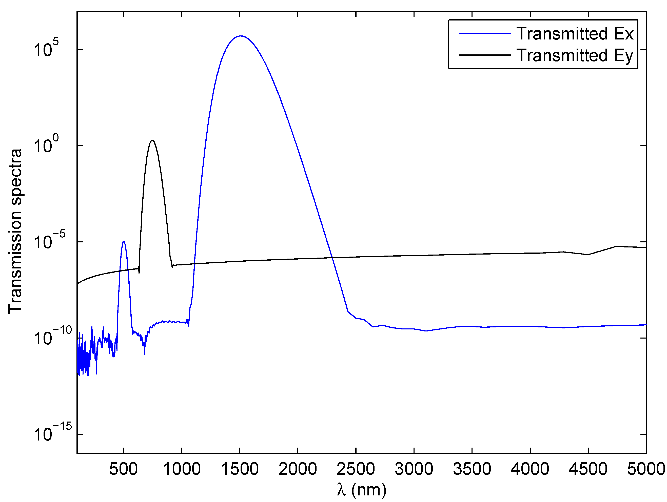
Figure 3, the wavelengths of
and
components are plotted after the Fourier transform. The conversion efficiency in our numerical simulation is calculated as
which is in good agreement with the experimental result (less than
as published in [
4,
5]). Good agreements are achieved between our numerical result and the experimental result.
Figure 2.
Time history of (a) the linear response, and (b) the nonlinear response, for U-shaped metallic particles illuminated by a x-polarized incident light.
Figure 2.
Time history of (a) the linear response, and (b) the nonlinear response, for U-shaped metallic particles illuminated by a x-polarized incident light.
Figure 3.
Semi-log plot of the Fourier transform of the time history of the far-field projection of the and components of the electric field as functions of the wavelength for U-shaped nanoparticles illuminated by a x-polarized incident light.
Figure 3.
Semi-log plot of the Fourier transform of the time history of the far-field projection of the and components of the electric field as functions of the wavelength for U-shaped nanoparticles illuminated by a x-polarized incident light.
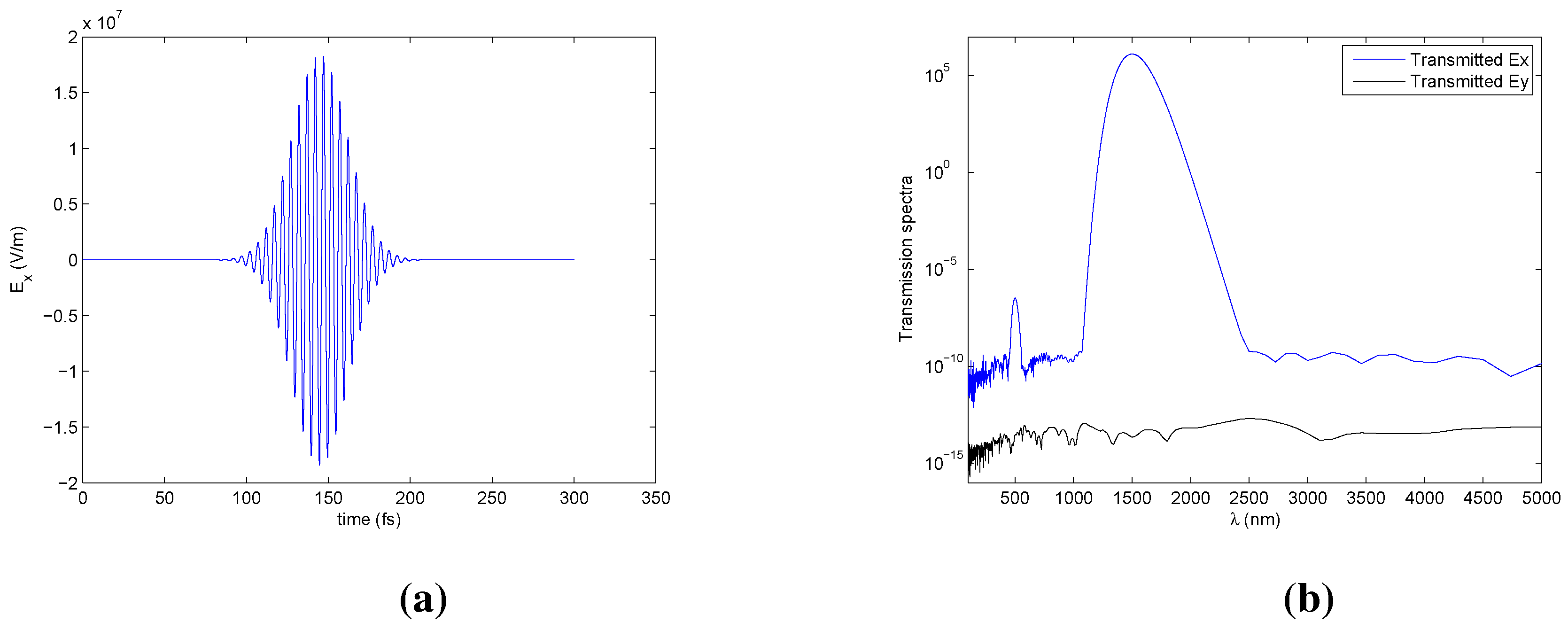
In the second simulation, we test our model for a rectangular shaped nanoparticle, and the corresponding results are shown in
Figure 4. The structure is similar to the rectangular shaped structure given in [
4]. Since rectangular shaped structure is symmetric in both
x and
y directions, there is no SHG, but there exists third harmonic generation (THG). Experimental results on third harmonic generation were published in [
4]. As shown in
Figure 4, our results confirm that no SHG is generated from rectangular nanoparticles and there is THG for both U-shaped (shown in
Figure 2) and rectangular shaped structures. The SHG from U-shape is much stronger than the rectangular shape, which is also in agreement with the experimental results published in [
4].
Figure 4.
(a) Time history of the linear response for rectangular shaped nanoparticle illuminated by a x-polarized incident light; (b) Semi-log plot of the Fourier transform of the time history of the far-field projection of the and components of the electric field as functions of the wavelength.
Figure 4.
(a) Time history of the linear response for rectangular shaped nanoparticle illuminated by a x-polarized incident light; (b) Semi-log plot of the Fourier transform of the time history of the far-field projection of the and components of the electric field as functions of the wavelength.
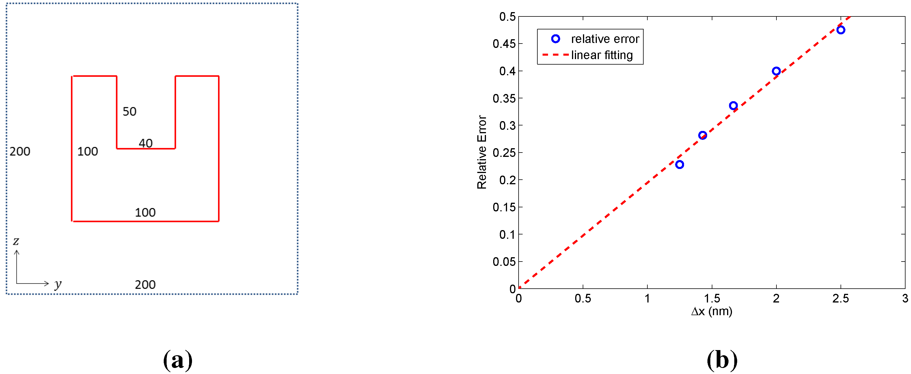
Figure 5.
(a) cross-sections of the U-shaped gold nanostructure with the unit of ; (b) the convergence test of the our numerical method for solving SHG strength.
Figure 5.
(a) cross-sections of the U-shaped gold nanostructure with the unit of ; (b) the convergence test of the our numerical method for solving SHG strength.
Furthermore, we test the convergence of our method using a smaller two dimensional structure shown in
Figure 5a. The U-shaped nanostructure is in
plane and infinitely long in the
x-direction. We use a uniform grid whose size varies from 2.5 nm down to 1.25 nm. A fine grid result with
is chosen as the reference solution. From the convergence test result shown in
Figure 5b, we conclude that our numerical method is convergent.
