M5GP: Parallel Multidimensional Genetic Programming with Multidimensional Populations for Symbolic Regression

Abstract

Machine learning and artificial intelligence are growing in popularity thanks to their ability to produce models that exhibit unprecedented performance in domains that include computer vision, natural language processing and code generation. However, such models tend to be very large and complex and impossible to understand using traditional analysis or human scrutiny. Conversely, Symbolic Regression methods attempt to produce models that are relatively small and (potentially) human-readable. In this domain, Genetic Programming (GP) has proven to be a powerful search strategy that achieves state-of-the-art performance. This paper presents a new GP-based feature transformation method called M5GP, which is hybridized with multiple linear regression to produce linear models, implemented to exploit parallel processing on graphical processing units for efficient computation. M5GP is the most recent variant from a family of feature transformation methods (M2GP, M3GP and M4GP) that have proven to be powerful tools for both classification and regression tasks applied to tabular data. The proposed method was evaluated on SRBench v2.0, the current standard benchmarking suite for Symbolic Regression. Results show that M5GP achieves performance that is competitive with the state-of-the-art, achieving a top-three rank on the most difficult subset of black-box problems. Moreover, it achieves the lowest computation time when compared to other GP-based methods that have similar accuracy scores.

1. Introduction

Genetic Programming (GP), first conceptualized over 30 years ago [1], was proposed as a general purpose problem solving paradigm, applicable to a wide variety of domains, from program synthesis to circuit design [2]. However, the most widely studied problem in GP has been Symbolic Regression (SR), a type of machine learning problem where the goal is to predict a real-valued output while also generating a symbolic and (potentially) human-readable model [1,3,4]. Indeed, a large variety of GP-based methods has been proposed for SR that have extended the originally proposed tree-based GP, incorporating specialized search techniques and sophisticated implementations [3,4]. While no broadly used taxonomy exists, there are some obvious ways in which to categorize GP-based SR methods and some of the aspects that could be taken into account are the following:

• Representation: the way in which solutions are represented (trees, graphs, arrays or stacks);
• Objectives: the number of objectives (single- or multi-objective), or the type of objectives used (error, correlation or novelty);
• Search process: how the method searches for or constructs a feasible model, including how the population is managed (for example, the use of single or multiple populations) or the type of search operators used (syntactic operators, semantic operators or hybrid techniques with local search methods);
• Search space: this is related to the set of feasible models that the technique can produce; i.e., the structure or the type of model than can be generated by the search process.

From a practical point of view, although not necessarily from the perspective of the search technique itself, the final aspect may be the most important [5]. While different types of models exist, there are at least two general groups of GP-based SR methods that could be identified: (1) unconstrained SR methods and (2) constrained SR methods. An unconstrained method can produce any type of model that is feasible given the primitive elements used to construct it. For a GP approach, feasibility would depend on the primitive elements used by the method and the size limit imposed by the search process (even if the size limit is merely based on the available system memory). For instance, this group of methods includes standard GP [1], stack-based GP [6], or memetic variants [7]. Conversely, constrained methods utilize additional rules that constrain what type of models can be produced, rules that go beyond what is included in the terminal and function sets. These rules could be imposed, for instance, during the genotype to phenotype mapping of a candidate solution [8], directly in the solution representation [9], or as part of the search operators used [10].

In particular, in recent years, there has been significant interest in using GP to generate models that are linear in parameters [11], hereafter referred to as linear models for simplicity. These models are of the form

$$y=w_0+w_1{x}_1+w_2{x}_2+\cdots +w_n{x}_n$$

(1)

where y is the output variable (target), $x_1$, $x_2$, $\cdots$, $x_n$ are the input variables (features), $w_1$, $w_2$, $\cdots$, $w_n$ are the model parameters (weights), $w_0$ is the bias term and $x_i,w_i,y\in \mathbb{R}$. Notice that, while these models are linear from the perspective of the parameters of the model, the individual terms can be nonlinear, such that a linear model can be posed as

$$y=w_0+w_1{K}_1\left(\mathbf{x}\right)+w_2{K}_2\left(\mathbf{x}\right)+\cdots +w_n{K}_d\left(\mathbf{x}\right)$$

(2)

where $\mathbf{x}=(x_1,x_2,\cdots ,x_n)$, $K_i:{\mathbb{R}}^n\to \mathbb{R}$ are linear or nonlinear transformations of the input features, also known as basis functions, and $i=1,\cdots ,d$ with d not necessarily equal to n. For instance, these functions can be polynomial expansions, radial basis functions, or wavelets, to name a few common variants.

One of the benefits of using linear models is that they are amenable to well-known statistical analysis and tuning [12]. Another benefit can be obtained when the transformation functions are relatively simple and symbolic in nature, potentially making model understanding and interpretation much more feasible [5,13]. Even with linear models, intepretability is often not possible when using kernel methods, for instance, when the number of parameters in those models grows with the number of observations, or ensemble methods that require a very large number of weak models. Moreover, similar issues arise with nonlinear black-box models, such as the Multilayer Perceptron (MLP). Therefore, the discovery of relatively simple transformation functions is desirable in many modeling tasks. Moreover, estimating model parameters can be carried out in a relatively simple and robust manner for these models, using matrix decomposition or gradient-based methods, that can facilitate model simplification with regularized techniques [14]. Conversely, parameter estimation in GP-based SR with traditional search operators is highly inefficient [15]. A final comment is that while most constrained SR methods focus on generating linear models, other types of constraints may be possible, such as focusing the search on ordinary differential Equations [16], dynamical system models [17], or time series models [18].

It may seem reasonable to assume that constrained methods will be at a disadvantage compared to unconstrained methods for some SR tasks. Simply put, if the underlying “ground-truth” model of a given dataset is not a linear model, then these approaches can only produce approximate solutions. However, this may not necessarily be a shortcoming. In some cases, a linear approximation of a signal may be preferable, even if a complex nonlinear model exists that more accurately describes the behavior of the signal. A linear model may be much simpler and easier to understand, and may still approximate the output with sufficient accuracy. Moreover, a linear model can, in theory, approximate any function with the appropriate basis functions [19].

For GP-based SR, however, both constrained and unconstrained approaches share an additional practical issue, their inherent and non-trivial computational cost [3,4]. In general, state-of-the-art SR methods that are based on GP search for both the structure of the model and tune model parameters. This increases the required computational cost and total runtime of the learning process. Therefore, new methods must account for this fact and design and implement the search accordingly. Most state-of-the-art GP-based methods are relatively slow, even highly efficient implementations cannot compare with traditional machine learning techniques [3,4]. This is particularly an issue for GP-based SR methods that generate linear models, since both syntactic and numerical optimization is required to estimate the model structure and parameters [4,9]. Indeed, probably the most efficient GP-based SR method, the Fast Function Extraction (FFX) algorithm, eliminated the evolutionary loop to reduce runtimes [3,4,20]. This allows FFX to be competitive with off-the-shelf modeling techniques based on efficiency [20]. Another recent example is PySR, which uses a multipopulation evolutionary search and improves search efficiency using a distributed approach [21].

The present work addresses the SR problem by proposing a new feature transformation method to build linear models, based on the previously proposed M2GP, M3GP and M4GP methods [9,22,23]. This new method is called M5GP, and it was designed to exploit parallel processing on a Graphical Processing Unit (GPU) by executing the main evolutionary processes on the GPU, including population initialization, evaluation, selection, variation and survival. Moreover, parameter estimation for each linear model is also performed using GPU processing. It is important to highlight, moreover, the fact that GPU-processing is not necessarily unique in machine learning systems, except for the subset of methods focused on SR-methods. This is particularly the case for those that employ a feature transformation approach, or those that are currently considered to represent the state-of-the-art [4]. M5GP combines the general workflow of M3GP [9] to produce models that perform feature transformation and then combine the transformed features to build linear models [24]. However, the proposal employs the solution representation of M4GP [23], along with a variation of the mutation operator for stack-based representations proposed in [25], which simplifies the encoding and search for multidimensional transformations of the input feature space. The proposed method also employs the GPU-based processing used in [26] for increased efficiency in the evolutionary process and parameter estimation of the resulting linear models methods with cuML [27]. M5GP is evaluated using the recently proposed benchmarking suite for SR called SRBench v2.0 [4]. This allows for direct comparisons with GP-based and non-GP methods that are considered to be the current state-of-the-art for SR. Comparisons are done based on accuracy, complexity (model size) and processing time, using an extensive set of black-box (with unknown ground-truth models) and white-box (with known ground-truth models) SR problems. Results show that M5GP, combined with standard multiple linear regression, can produce state-of-the-art results in SR. Moreover, given that the core element of M5GP is the feature transformation process, it can be hybridized with other regression methods, extended to other tasks (such as classification), and applied to new problems using a standard scikit-learn interface [28], downloadable as an open-source tool, at https://github.com/armandocardenasf/m5gp (accessed on 31 January 2024). The remainder of this paper proceeds as follows. Section 2 presents background and related works, focusing on constrained SR methods. Section 3 presents the proposed M5GP, including representation, evaluation, search operators, hyperparameters, fitness computation and parallel implementation. Section 4 presents the experiments, main results and a discussion, largely based on the SRBench v2.0 benchmarking suite. Finally, a summary and conclusions are given in Section 5.

2. Background

This section describes the methods on which M5GP is based, focusing on the main contributions introduced by each and highlighting their strengths and weaknesses. A brief overview of other constrained GP-based SR methods is also presented, methods that share some of the same design elements as M5GP.

In general, M2GP [22], M3GP [9,24], M4GP [23] and M5GP can be referred to as wrapper approaches for automatic feature transformation, which may also be referred to as feature construction, feature engineering, or the constructive induction of features [11]. This task is closely related to the problem of feature selection, where the goal is to select which features to use in order to train a predictive model [29]. While feature selection limits itself to choosing a subset of features, feature transformation can both select the best features to use and also generate new ones. The goal is to transform the feature space of a problem, such that the new representation allows for a more efficient and effective learning process to take place. Indeed, several state-of-the-art methods combine a feature transformation process with another modeling technique to implement a constrained SR method [20,30].

Feature transformation methods can be grouped into two general classes, filter or wrapper approaches. A filter method performs feature transformation without considering the effect on any particular learning algorithm, using general criteria to transform the feature space, for instance, by discarding highly correlated features or generating a new feature space based on the directions of maximum variance in the data. Conversely, wrapper methods perform the transformation using a feedback loop, in which the performance of a learning stage is used to guide the feature transformation process, as shown in Figure 1. A wrapper method is basically posing a search problem in which the goal is to find the best feature transformation that maximizes the performance (or minimizes the loss) of a particular learning method. In the case of feature selection, genetic algorithms, for instance, are popular techniques [31]. Meanwhile, GP has been used to develop both wrapper-based [9,22] and filter-based approaches [32].

Moreover, GP can be said to perform both tasks concurrently. In most cases, the terminal set of a GP method includes all the original features of a problem, but the final model produced often does not use all of the features, implicitly performing feature selection [33]. Moreover, in standard GP, each individual in the population normally produces as output a single value for each sample in a dataset. GP individuals are effectively mapping the n-dimensional feature space onto a single new feature. This output can be interpreted as the model prediction or as a new decision space on which a higher level model can be used to obtain the final prediction [34,35].

The methods that are reviewed next extend this basic idea, by evolving models that can produce more than one output for each sample in a dataset. They generate transformation models T of the form $T\left(\mathbf{x}\right):{\mathbb{R}}^n\to {\mathbb{R}}^d$. This multidimensional output can be interpreted as a transformation of the original feature space. When used as a wrapper approach, it can search for the best feature transformation for a particular problem and learning method. The transformation model is in effect a collection $T=\{K_i\left(\mathbf{x}\right):{\mathbb{R}}^n\to \mathbb{R}\}$ of d symbolic transformations $K_i$, each one producing a new feature dimension. A possible justification for such approaches has been recently published in [36], which suggests that GP-based search is better served by generating a large collection of shallow models instead of a single model that is both large and deep.

2.1. M2GP: Multidimensional Multiclass Genetic Programming

M2GP evolves transformations using a tree representation in which the root of the tree acts as a dummy node, such that it only serves as a container for the output of d subtrees rooted at the node [22]. In this way, each individual is better understood as a collection of d standard GP trees [1]. Each of these subtrees can also be referred to as the new feature dimensions for the evolved transformations. In the case of M2GP, d is set as a static hyperparameter of the algorithm. The search operators used by M2GP are standard subtree crossover and mutation. M2GP was conceived as a classification method, paired with the Mahalanobis distance classifier. Results showed that M2GP compared favorably with standard machine learning techniques, such as Random Forest (RF), Random Subspaces (RS) and MLP.

However, M2GP presents several limitations. First, the size of the transformed feature space d is set as a hyperparameter, and it is reasonable to assume that in most cases it is not easy to define this parameter optimally. Second, M2GP relies on standard subtree search operators, which do not take into account the multidimensional nature of the individual transformations. Third, it was only evaluated and applied to classification tasks without considering the application of the method to SR tasks. Finally, like most GP methods, M2GP is a relatively slow method, limiting its usefulness for machine learning practitioners that require efficient prototyping. This issue is made more glaring since it was implemented sequentially in Matlab, not exploiting the fact that evolutionary algorithms are intrinsically parallel.

2.2. M3GP: M2GP with Multidimensional Populations

M3GP was developed to address several of the issues of M2GP [9]. It uses the same solution representation but incorporates several search operators that are specifically designed to exploit the multidimensional nature of the evolved transformation. Specifically, M3GP includes a mutation operator that can add a new subtree to the root node and another that can randomly delete a complete subtree from the root node. These operators effectively add or remove new feature-space dimensions to the evolved transformations. For crossover, M3GP adds a crossover operator that focuses on exchanging complete feature dimensions between two parents. M3GP also adds a local search operator called pruning, which eliminates feature dimensions from the best individual of the population until performance degrades. Indeed, due to the type of representation being used, these types of operators are also used by similar techniques [30]. These operators address the second issue with M2GP.

Another difference with M2GP is that all the individuals in the initial population begin with uni-dimensional transformations, with $d=1$. Mutation is the mechanism by which new feature dimensions are added, without an a priori limit, addressing the first issue with M2GP. On classification problems, M3GP outperformed M2GP and performed as well as RF and better than RS. Moreover, M3GP has been combined with other learning algorithms, not just the Mahalanobis distance [37]. That work showed that M3GP can improve the performance of a wide variety of classifiers, including naive Bayes, Support Vector Machines, RF and XGBoost [38].

Unlike M2GP, M3GP has also been applied to regression tasks [24], in combination with multiple linear regression. For simplicity, multiple linear regression is referred to as linear regression hereafter. On both synthetic and real-world datasets, M3GP achieved very high accuracy, outperforming other GP-based methods. In particular, in comparison with FFX [20], M3GP produced similar performance but was able to generate much more compact—and potentially interpretable—models. On both regression and classification, M3GP showed an ability to dynamically and effectively adapt the number of dimensions for the evolved feature-space transformations [24,37]. The strong performance of M3GP on classification and regression has lead to work in other domains, such as extending M3GP for the analysis of complex signals [39,40,41].

There are, however, at least two important issues with M3GP, which also affect M2GP. First, by relying on a tree-based representation for the evolved transformations, it inherits all of the difficulties that stem from using this representation to evolve a solution, particularly since other representations have been shown to be more amenable to evolutionary search [6]. By relying on a tree representation, for instance, a special root node had to be defined, with special considerations regarding its interpretation and manipulation during the search. Second, the two most popular implementations of the algorithm, one in Matlab (https://github.com/LuisMuDe/M3GP_Regression) and the other in Python (https://github.com/jespb/Python-M3GP), usually have very long runtimes, not unlike some of the most efficient GP-based approaches to SR [3,4]. This is partially due to the fact that M3GP is a wrapper method that has to train an additional machine learning model at every fitness evaluation. Another reason is that none of the previous implementations exploit the massively parallel capabilities of modern GPUs; although it should be noted that the Python implementation does include multiprocessor computations.

2.3. M4GP: Incorporating a Stack-Based Representation

The latest variant of M2GP is aptly named M4GP, introducing several notable improvements [23]. First, M4GP changes the program representation using a linear genome and stack-based interpretation of the models. The genome is a linear sequence of primitive elements (functions and terminals), which are interpreted sequentially using an auxiliary stack. When the interpreter reaches a terminal gene, it pushes it onto the stack, and when a function gene is processed, the necessary operands are popped (pulled) from the stack, and the results is pushed back to the stack. When an operation cannot be performed, it is simply skipped and the stack is returned to its previous state. For instance, when the stack does not contain sufficient values for a particular function to be executed.

Such a representation is not new or unique. For instance, a similar representation is used for efficient GPU-based implementations of GP that have used a postfix reverse polish notation for GP trees [42] or a Linear GP representation [43]. Such representations are more amenable to parallel processing on a GPU but require special search operators and initialization techniques in order to guarantee well formed expressions. M4GP, based on PushGP [6], need not account for this issue, with individual models often leaving the stack with more than a single value after the entire genome has been evaluated.

Taking the top element in the stack as the output seems reasonable for a standard GP approach, but the entire stack could be used to obtain a multidimensional output for free. Since the representation does not force the programs to be a single complete expression, and since programs will produce stacks of different sizes, M4GP achieves the same functionality as M3GP with a much simpler algorithm.

The initial population is initialized recursively, generating programs of different sizes and feature dimensions, unlike M3GP, which starts with unidimensional populations. Three different selection schemes were evaluated, namely the standard tournament selection, lexicase selection [44] and age-fitness Pareto [45]. The search operators used by M4GP are equivalent to those used in M3GP, assuming that such operators may have an intrinsic value for the search process. In general, M4GP outperforms M3GP on a wide variety of classification tasks, and is very competitive with other machine learning techniques, including Adaboost, SVM and XGBoost. It is also able to outperform more powerful classifiers based on Auto Machine Learning (AutoML) [46]. Finally, M4GP is the first variant to include parallelism during the search, using an island model that processed subpopulations on different CPU cores of the host machine, with improved runtimes.

M4GP was a notable improvement over M3GP, but several promising lines of research are still unexplored. First, M4GP, like M2GP, was only applied to classification tasks, SR problems were not considered. Second, like all GP-based methods, runtime is still an issue for the method, even with the implemented island model. Moreover, while such an approach did help reduce runtimes it added additional hyperparameters to the algorithm. Finally, the search operators used were inherited, in a sense, from the tree-based representation of M3GP, instead of using search operators specifically designed for the representation used.

2.4. Related Work

While the previous subsections focused on the methods that are most closely related to M5GP, this subsection briefly outlines some of the most relevant state-of-the-art SR methods that are also based on GP. The recently proposed SRBench benchmark suite [3,4], presents the most comprehensive, systematic and reproducible evaluation process for SR algorithms. While SR is the most widely studied problem in GP, assessing and comparing SR methods was mostly done in an ad hoc manner before SRBench [47,48]. Moreover, it provides open-source and easy-to-use implementations of the state-of-the-art methods, considering both GP and non-GP methods.

Among them, several unconstrained methods achieve the highest overall performance. For instance, Operon, which produces the most accurate and relatively compact models, implemented in a highly efficient manner [7]. In fact, while Operon runs on a CPU, its multithreaded implementation allows it to be more efficient than some FPGA- and GPU-based implementations [49].

Another unconstrained method that achieves high accuracy is Semantic Backpropagation GP (SGP) [50]. Implemented using a tree-based representation, SGP recursively determines the best subtree to insert into a program tree, selecting from a library of available trees. The output of any particular tree or subtree is referred to as the semantics of the tree, so SBP searches for the best possible match between the available semantic vectors and the optimal semantic vector at any particular node of a tree. While this method achieves very high performance, it suffers from very long runtimes and produces larger models than other GP-based approaches.

Constrained SR methods that produce linear models include Geometric Semantic Genetic Programming (GSGP) [10], Kaizen Programming [51], Multiple Regression GP [8], Interaction-Transformation Evolutionary Algorithm (ITEA) [52], FFX [20] and Feature Engineering Automation Tool (FEAT) [30], with MRP, ITEA and FEAT all included in SRBench. FFX, for instance, does not use an evolutionary loop and instead generates a very large initial population (set) of basis functions and combines all of them into a final model, pruning the model with regularized regression. Kaizen Programming also builds a single model using the entire population, and substitutes the traditional evolutionary process with another metaheuristic. GSGP builds a linear model in a step-wise manner, with each mutation or crossover event adding a new term to each parent program. MRGP generates a model by linearly combining a GP individual with a subset of the subtrees it contains. ITEA imposes restrictions on the form of the basis functions that are included in the model, biasing the search with the expectation that simpler and more interpretable models are produced.

Among these, FEAT achieves the best performance and shares several similarities with M3GP and M4GP. It models the evolved transformations using a network structure and uses a syntax tree representation. Search operators are similar to those of M4GP but include a feedback loop to determine the best place to apply the mutation operator. Similar to M4GP, it uses lexicase selection and a Pareto criterion during survival to promote the production of smaller models.

From the SRBench results, three observations can be highlighted. First, among all methods, GP-based approaches achieve the best performance, with Operon, SBP and FEAT producing the most accurate models. Second, in terms of size, standard machine learning ensemble methods produce very large models, as does FFX. GP-based methods in general tend to produce relatively small models. The main issue with GP-based methods is runtime, with only FFX achieving competitive performance in this respect compared to non-GP techniques, which is made possible by its lack of an evolutionary loop. Moreover, all of the methods are implemented for execution on CPUs. None of the GP-based methods exploit the massively parallel GPU platforms that have become the norm in large-scale machine learning tasks.

3. GPU-Based Parallel Implementation of M5GP

This section presents the core elements of M5GP, which as previously discussed, contains elements of both M3GP and M4GP, while utilizing some of the design choices used in the recently published CUDA-based GSGP-CUDA [26]. M5GP was developed using Python v3.9.12, using GPU processing with Numba kernels [53] and cuML [27] kernels for parameter estimation. To summarize, the main design elements of M5GP are as follows:

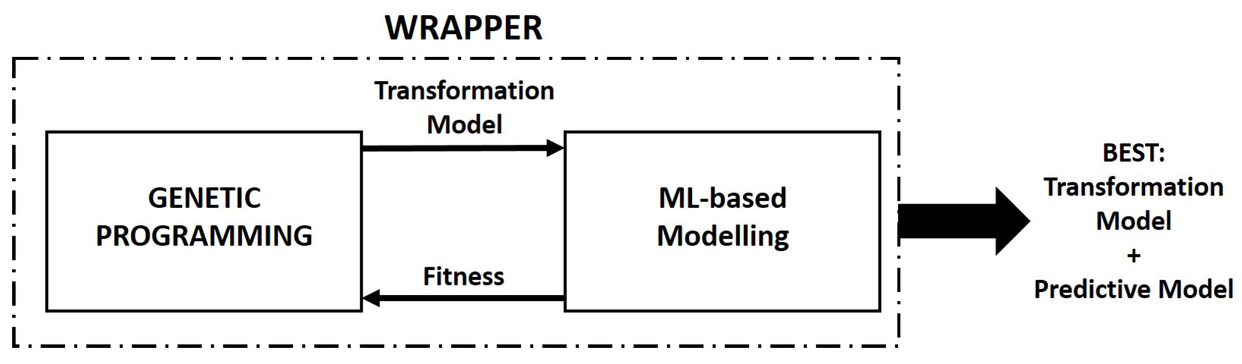
• The main evolutionary loop is controlled using Python code executed on the CPU but each of the main evolutionary processes are executed on the GPU, including population initialization, program evaluation done by an interpreter, selection and mutation;
• Individuals are encoded using a linear representation, basically initialized as a list of randomly ordered primitives (terminals and functions). The individuals are considered to be transformation functions of the input feature space of a problem;
• Individuals are interpreted using a stack. Since most individuals will encode a set of sub-expressions, they tend to produce stacks of different sizes, the transformed feature space of the training data;
• The mutation operator used by M5GP is based on the Uniform Mutation by Addition and Deletion operator (UMAD) [25] and selection is performed using tournaments. The former was chosen because it has been shown to produce strong results with stack-based GP, while the latter was chosen instead of more advanced methods (such as lexicase selection [44] used by M4GP) for simplicity and efficiency purposes;
• All of the evolutionary processes in M5GP are implemented as GPU kernels using Numba, except for parameter estimation which is carried out using linear regression with cuML;
• Linear models are constructed using the output stacks of each individual using cuML, and the Root Mean Squared Error (RMSE) of the model is returned as fitness;
• M5GP returns the best feature transformation model and the corresponding linear model fitted using the cuML library;
• For ease of use, M5GP implements the scikit-learn API, allowing it to be evaluated on SRBench [4].

3.1. Individual Representation, Interpretation and Parallel Processing

Individuals in M5GP, each one encoding a feature transformation, are encoded as fixed-length linear sequences of primitive elements, following [26]. Terminals include each of the original problem features (model inputs) $x_1,x_2,\cdots ,x_n$, as well as random constants in the range $[a,b]$. The function set contains: $+,-,*,AQ,sin,cos,log,exp,abs,NOOP$. The NOOP operator is included to allow individuals to encode fewer functional operations than their maximum length, and also to allow the transformations to shrink or grow during the search process, a common feature of most GP-based systems. A specific probability is assigned for the generation of each function (gene function probability), terminal (gene variable probability), constant (gene constant probability), or NOOP operator (gene NOOP probability); the values used are shown in Table 3.

The $log$ operator is protected, acting as a NOOP when the input is a negative value. Instead of the protected division, the analytic quotient operator is used, which is defined as $AQ(a,b)={\displaystyle \frac{a}{\sqrt{1+b^2}}}$ [54]. The analytic quotient removes discontinuities or singularities from the evolved expressions, which often arise when the protected or unprotected division are used to evolve regression models. It also has been shown to improve performance on regression tasks [54].

Figure 2 shows a small population of individuals, each one randomly generated on a single processing thread using a Numba kernel. For the random generation of the genes of each individual, different probability values are assigned to include functions, features, or constants. In the experiments, a probability of 0.5 was assigned for functions, 0.39 for variables, 0.1 for constants and 0.01 for NOOP operators. In general, this produces large individuals that can then be pruned by the mutation operator.

After initialization, each individual is evaluated on each training sample (fitness case) in the training dataset. M5GP uses the same interpreter reported in [26]. Starting from the first gene or element in an individual, if it is a terminal element (feature or constant), it is pushed onto an output ${\mathbf{x}}^{\prime }$. If it is an operator from the function set of arity a, then a pull (also known as pop) operations are performed on the stack and the pulled values are used as inputs to the operator, and the output is then pushed onto the output stack. Only for the best individual at each generation, for efficiency purposes, is the subexpression that generates each element in the output stack also pushed onto an expression stack. This process is depicted in Figure 3 for the top individual in Figure 2. The entire process is based on [23].

After interpreting an individual i on training sample j, the result is an output stack ${{\mathbf{x}}_{\mathbf{j}}^{\prime }}^{\mathbf{i}}=(x_{j,1}^{\prime i},x_{j,2}^{\prime i},\cdots x_{j,d}^{\prime i})$ of size $d\le l$ with l the size of the individuals in the population, but most of the time, d is much smaller than l. The output stack can also be interpreted as the semantics of the individual evaluated on a single fitness case, which is often considered as a scalar value [10], but in M5GP (as well as M4GP) it is an array. This also defines the size of the new feature space for the problem. Therefore, after evaluating an individual transformation model on the entire training set with m samples, and considering each ${\mathbf{x}}_{\mathbf{j}}^{\prime \mathbf{i}}$ as row vectors, this produces an output that is referred to as the semantic matrix of individual i, defined as

$${S_i}_{m\times s}=\left[\begin{array}{c}{\mathbf{x}}_{\mathbf{1}}^{\mathbf{\prime }\mathbf{i}}\\ {\mathbf{x}}_{\mathbf{2}}^{\mathbf{\prime }\mathbf{i}}\\ ⋮\\ {\mathbf{x}}_{\mathbf{m}}^{\mathbf{\prime }\mathbf{i}}\end{array}\right].$$

(3)

The semantic matrix contains the new feature space representation of the training data. The entire process is executed on the GPU using Numba kernels, as depicted in Figure 4.

The development of a GPU-based implementation of any algorithm can be successful if it is able to maximize the usage rate of the resources on the GPU card. The interpreter kernel processes individuals on independent GPU threads, with the grid size and block size computed based on the GPU characteristics. The total amount of shared memory is determined and reserved based on the size of the dataset and the size of the individuals and the population to store the individual genotypes as well as the semantic matrices produced by the interpreter. The memory required to store the population is proportional to $pop\times l$, where $pop$ is the population size and l is the length of the individuals. The memory allocated to the semantic matrices of the entire population is proportional to $pop\times l\times m$, where m is the number of samples or fitness cases in the training set. If the amount of memory required by the population, the semantic matrix and the training data exceeds 85% of the available memory on GPU, then the population and data are processed in batches, to allow for additional processes required.

The semantic matrices returned by the Numba kernel are stored in an array, and need to be divided and reshaped into a cuPy matrix [55] for each individual before they are passed to the cuML functions. The current implementation performs this conversion on the CPU before passing the transformed dataset to cuML. The cuML regression functions return the linear model for each M5GP individual but do not return the training error or other statistics. Inference on the training data has to be performed and the error computed to assign fitness.

3.2. Fitness Evaluation Using CUDA-Based Machine Learning

Using the semantic matrix of each individual, a linear regression model is fitted such that the final model is given by a linear combination of the d expressions in the corresponding expression stack, as defined in Equation (2). Using the expression stack and the $d+1$ model coefficients, $w_0,w_1,\cdots w_d$, the final regression model for each individual can be reconstructed.

To fit the regression models, cuML was used, and this suite of machine learning libraries was specifically implemented in CUDA. It was developed as part of the RAPIDS project https://rapids.ai/ (accessed on 31 January 2024). The library offers a wide range of common machine learning algorithms that run efficiently on GPU cards and can potentially scale to multinode and multi-GPU processing with Dask https://www.dask.org/ (accessed on 31 January 2024). The fitness value for each individual is defined by the RMSE of the cuML model evaluated on the training data, as done previously with M3GP using linear regression models [24]. For experimental purposes, several linear regression methods included in cuML were evaluated with M5GP, such as regularized regression approaches and mini-batch approaches. However, as will be shown in the experimental section, the best results were obtained using Singular Value Decomposition (SVD) decomposition with Jacobi iterations.

In principle, using a single GPU, as was the case in our experimental setup, it is possible to launch several cuML process in parallel using different CPU computing threads. However, the initial experimental tests showed a decrease in efficiency. Therefore, fitness evaluation is executed sequentially at the population level, but the parameter estimation process is executed using parallel computing on the GPU.

3.3. Search Operators

M5GP uses tournament selection, which is also implemented as a Numba kernel. However, the main novelty in M5GP, particularly when compared to similar approaches [4], is the use of a mutation operator based on UMAD [25]. For parent selection, the size of the tournament was set as a proportion of the total size of the population.

The logic of the UMAD operator is straightforward, it adds new genes, before or after existing genes, and then it randomly deletes genes from the resulting individual. The UMAD operator attempts to decouple the location where new genes are added from the location where older genes are removed, unlike most mutation operators that perform some form of gene replacement. Since M5GP uses a fixed length representation, it would be cumbersome to include an addition operation instead of a replacement operation. However, including an additional deletion-only operation can be quite useful to promote smaller models. The replacement operation of each gene uses the same probabilities for functions and terminals that were used in the initialization process, given in Table 3.

In this sense, M5GP performs a uniform mutation by replacement and deletion of each gene in an individual, where deleting a gene means replacing it with a NOOP terminal. Each gene is deleted with probability deletionRate and replaced with probability replacementRate. After several informal tests, best performance was achieved with a replacementRate of $0.1$ and a deletionRate of $0.01$. Mutation is applied to all selected individuals, and when a gene is replaced, it is chosen using the same probabilities used during population initialization. These values were validated based on the results reported for UMAD [25], which uses an addition rate instead of a replacement rate, but best performance was observed with similar values.

4. Experiments

SRBench v2.0 [4], which has been released as an open-source tool (https://github.com/cavalab/srbench) (accessed on 31 January 2024), is used to evaluate M5GP. SRBench v2.0 contains two groups of problems, 122 black-box regression problems from the PMLB v1. https://epistasislab.github.io/pmlb/ (accessed on 31 January 2024) repository [56], consisting of 46 real-world problems from diverse domains and 76 synthetic problems. It also includes 130 datasets with known model forms that can be used as a ground truth to compare the models produced by an SR method. For these problems, various datasets are generated by adding different levels of noise to the data. Dataset size varies from 47 to 1 million instances, and from 2 to 124 problem features. Datasets are split using 75/25% training/testing splits, and for black-box regression problems, each algorithm is tuned using hyperparameter optimization.

The methods in SRBench are compared using three main criteria. For the black-box problems, accuracy is evaluated using the coefficient of determination $R^2$. Complexity of the models is evaluated indirectly using the size of the symbolic expressions, defined by the number of functions and terminal elements contained in the models. Execution time is used to evaluate the computational efficiency of the methods.

SRBench includes both SR methods and state-of-the-art machine learning methods that do not produce symbolic models. The latter group includes nine methods, including XGBoost (XGB) [38], AdaBoost [57], Light Gradient Boosting Machine (LGBM) and RF [58]. In the former group, SRBench includes 14 relatively recent methods, with 8 of the methods published in 2019 or 2020. It includes both evolutionary and non-evolutionary approaches. Some notable examples include Operon [7], GOMEA [59] and DSR [60]. Operon achieves the best performance among all methods, while GOMEA shows the best compromise between accuracy and model size. Conversely, DSR tends to produce very compact models, but with lower accuracy. While some of the GP-based methods, like Operon and GPlearn (https://gplearn.readthedocs.io/en/stable/index.html) (accessed on 31 January 2024), do allow for multithreaded processing, none of them were developed to exploit modern GPUs, the current standard of massively parallel devices. Moreover, while GP-based systems that run on GPUs are not new [26,42,43], they mostly implement basic GP-based algorithms that do not perform as well as the current state-of-the-art.

4.1. Experimental Setup

This section describes how SRBench was used to evaluate different configurations of M5GP, and compare it with the methods provided in the benchmark suite.

In all, 12 configurations of M5GP were evaluated; these are summarized in

Table 1. Different M5GP configurations used for experimental evaluations.

Identifier	Regression	Tuning	Population	Genes	Fitness
M5GP-1	LR	Yes	256	128	RMSE
M5GP-2	LR	No	256	128	RMSE
M5GP-3	LR-n	No	256	128	RMSE
M5GP-4	LR	No	256	256	RMSE
M5GP-5	LR	No	256	512	RMSE
M5GP-6	LR	No	512	256	RMSE
M5GP-7	LR	No	256	128	$R^2$
M5GP-8	LR-m	No	256	128	RMSE
M5GP-9	LASSO	No	256	128	RMSE
M5GP-10	LASSO	No	512	256	RMSE
M5GP-11	EN	No	256	128	RMSE
M5GP-12	EN	No	512	256	RMSE

. M5GP-1 uses hyperparameter tuning, as done for all the methods in SRBench [4], to determine the best configuration from among those considered in

Table 2. Hyperparameters considered in the tuning of configuration M5GP-1; each row is one configuration.

Generations	Population	Genes	Tournament Size
30	128	128	0.25
30	128	128	0.15
30	256	128	0.1
30	256	256	0.1
50	128	128	0.25
50	128	128	0.15

. In particular, the tuning process is done using 5-fold halving grid search cross-validation [4]. As stated before, parameter estimation for the linear models is performed using cuML [27], and in all cases, default settings were used. In some cases, these hyperparameter configurations might not produce the best results, but tuning the hyperparameters of the cuML methods is left as future work. Moreover, current implementations in cuML do not compute the regularization path of the coefficients to determine the optimal $\alpha$ hyperparameter of the regularized techniques. M5GP-1 to M5GP-8 use linear regression, with LR denoting parameter estimation with SVD decomposition using Jacobi iterations and correction for the global mean of the output. LR-n is similar to LR but with normalized data and LR-m uses minibatch processing; normalization is accomplished by dividing by the column-wise standard deviation. All methods are from the cuML library. For LR, the intercept is fitted, correcting for the global mean of the output. Least Absolute Shrinkage and Selection Operator (LASSO) regression uses $\alpha =1$ for the L1 term; the solver is coordinate descent with 1000 iterations with cyclic parameter updates and correction for the global mean of the output. Elastic Net (EN) regression corrects for the global mean of the output, $\alpha =1$, L1 ratio of 0.5, coordinate descent solver, with 1000 maximum iterations and random selection, and a tolerance of 0.001. For LR-m, $\alpha =0.0001$, adaptive learning rate, using correction for the global mean of the output and a batch size of 1024.

M5GP-2 to M5GP-12 use fixed hyperparameter values, since previous works have shown that GP-based methods tend to be highly robust to hyperparameter settings [61,62]. Special cases include M5GP-3, which uses normalized data, M5GP-7, which uses $R^2$ for fitness and, as mentioned above, M5GP-8, which uses minibatch processing. All other variants use different amounts of search intensity, controlled by the number of genes (size of the individuals) and the population size. M5GP-9 to M5GP-12 use regularized regression, with M5GP-9 and M5GP-10 using LASSO regression and the rest using EN regression.

The shared hyperparameters used by most M5GP-1 variants are summarized in

Table 3. Shared hyperparameter values across all M5GP configurations from Table 1.

Hyperparameter	Value	Description
Generations	30	Iterations in the evolutionary loop
Function set	$+,-,*,AQ,sin,cos$$log,exp,abs$	Applied at the gene level
Terminal set	constants and features	Constants are in the range of $[-999,999]$
Replacement rate	0.1	Applied at the gene level
Delete rate	0.01	Applied at the gene level
Tournament size	0.15	Percentage of the population that will be included in the tournament
Gene function probability	0.50	Probability to choose a function during mutation or population initialization
Gene feature probability	0.39	Probability to choose a feature during mutation or population initialization
Gene constant probability	0.1	Probability to choose a constant during mutation or population initialization
Gene NOOP probability	0.01	Probability to choose a NOOP during mutation or population initialization

, with a brief description of their role. In the case of M5GP-1, the tuning process considered specific hyperparameter combinations, which are listed in Table 3. SRBench uses six hyperparameter configurations during tuning [4].

For the experiments, M5GP was executed on a desktop computer with an Intel(R) Xeon(R) CPU E5-2603 v4 @ 1.70GHz (Intel, Santa Clara, CA, USA) and 16 GB of RAM, an NVIDIA Quadro P4000 GPU with 1792 CUDA cores and a base frequency of 1506 MHz, which also has a boost frequency of 1480 MHz, and 8 GB of GDDR5 memory with a 256-bit memory interface with a bandwidth of 243 GB/s. Conversely, the results reported by SRBench were obtained using a heterogeneous cluster computing environment composed of hosts with 24–28 cores with Intel$\left(R\right)$ Xeon$\left(R\right)$ E5−2690 v4 @ 2.60GHz processors and 250 GB of RAM [4].

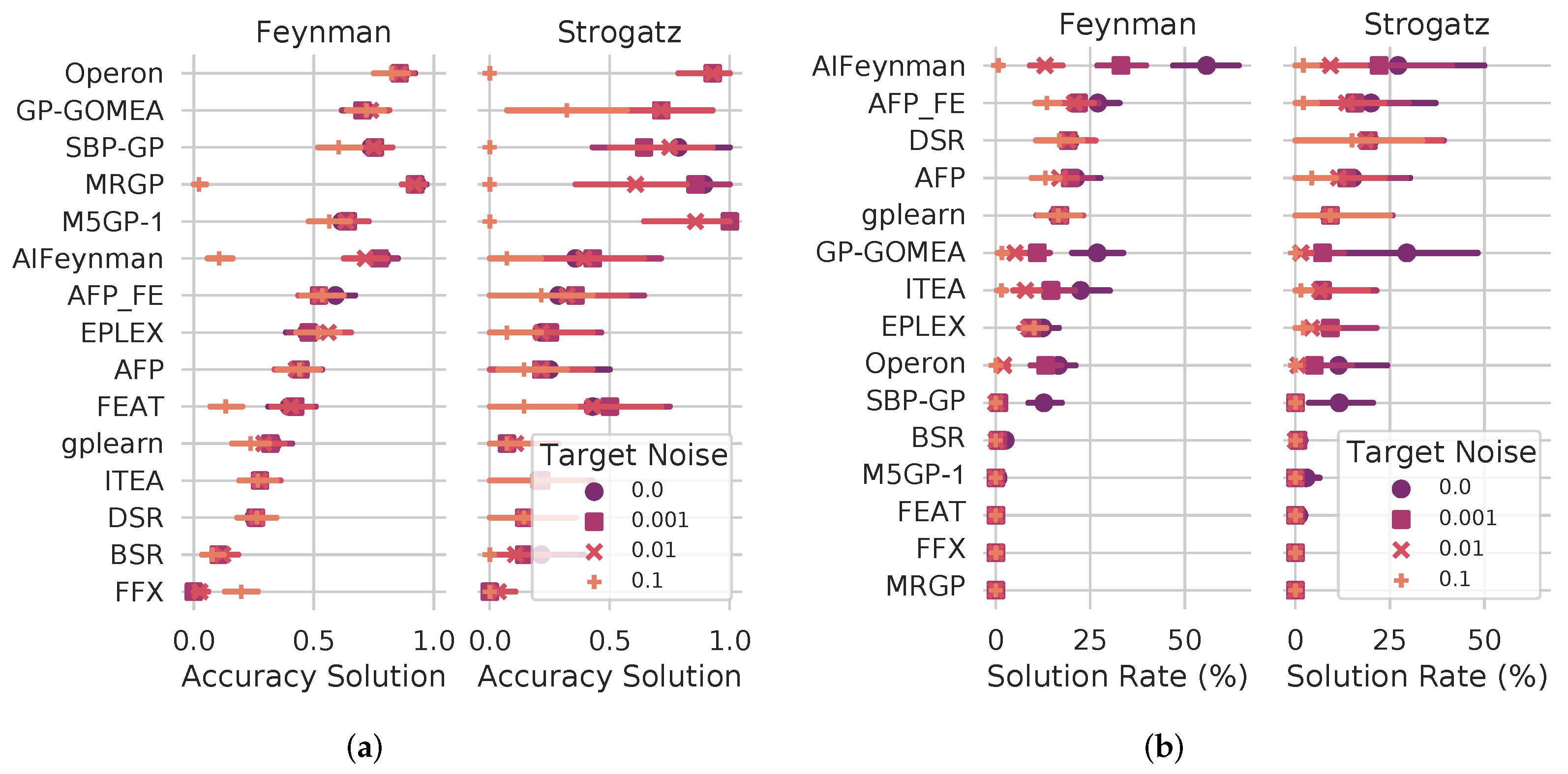
4.2. SRBench Results

This section presents the results obtained through SRBench, with comparisons between the different M5GP configurations and those obtained by the other methods included in the benchmark suite. Results are presented for both types of problems included in SRBench, black-box problems and ground-truth problems. Regarding computation time, the following must be considered. M5GP is the only method that uses GPU-based processing. While it is natural to expect that a GPU-based implementation will require less wall-clock time than a CPU implementation, this is not necessarily the case. Indeed, recent works have shown that CPU-based GP systems, such as Operon, for instance, can outperform GPU and FPGA implementations of [49,63]. Concerning model size, for the black-box problems, the methods in SRBench have not been configured to perform symbolic simplification of the models before computing model size.

Figure 5 presents the results from all the M5GP configurations summarized in Table 1. The methods in SRBench are evaluated based on: (a) $R^2$ test set performance, (b) model size (operators and operands in the model), and (c) total runtime during training. The plots show the median of the median performance across all problems (the median performance over all runs is computed, and the median of those values, over all problems, is shown in the plots), and bars indicate 95% confidence intervals. For each figure, the methods are ordered from the highest to the lowest rank, which is based on each performance measure.

Table 4. Median performance by all M5GP configurations evaluated on SRBench.

Identifier	${\mathit{R}}^2$	Model Size	Training Time (s)
M5GP-1	0.880	261.75	166.77
M5GP-2	0.822	234	150.89
M5GP-3	0.834	210.5	155.66
M5GP-4	0.840	444	231.81
M5GP-5	0.815	831	374.51
M5GP-6	0.584	1600	631.66
M5GP-7	0.713	234.5	132.32
M5GP-8	0.570	205	106.28
M5GP-9	0.544	203.5	119.18
M5GP-10	0.706	54.5	397.40
M5GP-11	0.325	19.5	141.09
M5GP-12	0.627	365	222.92

presents the median scores shown graphically in Figure 5.

From the results in Figure 5, the following can be stated. First, the top six methods in terms of $R^2$ all use LR, with regularized approaches (LASSO and EN) performing worse. This was unexpected, given previous results with regularized approaches used in FFX and MRGP, for instance [8,20], but may be due too poor hyperparameterization of the methods, since these tests use default values. Most variants have stable performance across the problem set, with only M5GP-6 showing large confidence intervals. It is of note that this configuration also uses LR, but with large individuals and a large population. The best performance was achieved using hyperparameter tuning (M5GP-1), but the difference with the best static hyperparameter setting (M5GP-4) is small, suggesting that if the available training time or computational resources are restricted, good performance can be achieved with a default configuration. Normalization does not seem to have a large impact on performance, as M5GP-2 and M5GP-3 are quite similar. Similarly, increasing the number of genes, the size of the individuals, has only marginal performance gains, with M5GP-2, M5GP-3 and M5GP-4 all achieving similar performance. In fact, increasing the size too much decreases performance, as seen by the drop-off in $R^2$ for M5GP-5.

The worst performance is exhibited by configurations M5GP-6 to M5GP-12. This selection includes all regularized regression variants (with LASSO or EN), the mini-batch variant (M5GP-8) and the variant that uses $R^2$ as fitness measure. Moreover, M5GP-6 uses the largest populations and individuals. This suggests that basic linear regression, without regularization, and relatively small populations and individuals achieve the best results.

In terms of model size, the effect of regularized regression is notable, with regularized variants producing the most compact models. There does seem to be a trade-off between achieving high accuracy ($R^2$) and producing compact solutions. However, apart from the extreme part of the plot, at the top and bottom of Figure 5b, about half of the M5GP configurations generate very similar models in terms of size, including some of the best-performing variants, such as M5GP-1, M5GP-3 and M5GP-2. M5GP-4, which is the best-performing variant that does not use hyperparameter optimization, does generate larger models since it uses larger individuals with 256 genes.

In terms of runtime, the most efficient variant was, as expected, M5GP-8, which uses mini-batch processing. Apart from that, it is clear that the most important factor affecting runtime is the number of genes, with runtime increasing in three different groups, with variants that use 128, followed by those using 256 and finally, the largest runtimes appear on the variants using 512 genes. Another factor is population size, the three slowest variants use populations of 512 individuals, which was expected since evaluating individuals is one of the most computationally expensive operations.

Figure 6 compares M5GP-1, M5GP-2, M5GP-3 and M5GP-4 with all other methods in SRBench. It is important to note that M5GP-1 is the only one that uses hyperparameter optimization, which is also the case for all other methods from SRBench included in the comparison. The good performance of the latter three methods is encouraging, since it shows that competitive performance can be achieved without costly hyperparameter optimization. M5GP-1 is similar in performance compared with FEAT, achieving the fourth rank in terms of $R^2$, while outperforming state-of-the-art methods like EPLEX, XGB and GP-GOMEA, to name a few.

In terms of model size, M5GP variants are in the middle of the pack, all very similar, producing more compact models than SBP-GP but larger models than methods such as ITEA, FEAT and Operon. In terms of training time, it is clear that exploiting parallel processing in GPUs allows M5GP to be very competitive, outperforming all other GP-based approaches and achieving similar runtimes to those of FFX and XGB.

Figure 7 presents a more detailed analysis of the results in Figure 6, but only considering M5GP-1. These plots show the matrix of p-values from the pairwise Wilcoxon signed-rank test, corrected for multiple comparisons using the Bonferroni method and considering a significance of $\alpha =0.05$. The null hypothesis of the Wilcoxon signed-rank test is that two groups share the same median. The results from Figure 6 and Figure 7 are complementary, since the latter allows us to discern which of the differences seen in the former are statistically significant.

Based on the statistical analysis, M5GP-1 shows equivalent performance, in terms of accuracy, to FEAT, along with other methods ranked below both, which include EPLEX, GP-GOMEA, LGBM, XGB and RF. It is clear that all of these methods have similar performance, in a second tier below Operon and SBP-GP. However, it is important to note that both Operon and SBGP-GP exhibit longer runtimes than M5GP.

Figure 8 presents the results for M5GP-1 in more detail, differentiating between what are referred to as the Friedman synthetic benchmarks, a special subset of problems that differ in degree of noise, variable interactions, variable importance and degree of nonlinearity [4]. These results show that M5GP-1 performs quite well on this subset of problems, that has been shown to be an important differentiator between the top-performing methods [4]. M5GP-1 slightly outperforms FEAT and notably outperforms XGB and most other methods, except for Operon and SBP-GP.

SRBench also includes two subsets of ground-truth SR problems, 130 in total. For these problems, the benchmark includes a known model, the symbolic ground-truth model. The two sets are the Feynman Symbolic Regression Database (https://space.mit.edu/home/tegmark/aifeynman.html) (accessed on 31 January 2024) and the ODE-Strogatz repository (https://github.com/lacava/ode-strogatz) (accessed on 31 January 2024). For these datasets, besides accuracy, SRBench uses the solution rate, i.e., the percentage of problems for which the ground-truth model was found, or a symbolic equivalent that differs from the true model by a constant or scalar factor. Moreover, for these problems, the methods are evaluated considering different levels of white Gaussian noise in the data, added as a fraction of the signal root mean square value, with noise levels of $[0,0.001,0.01,0.1]$. Figure 9 presents the results of M5GP-1 on the ground-truth problems, showing the accuracy using $R^2$ and the solution rate. The results In terms of accuracy, shown in Figure 9a, shows that M5GP-1 performs very well, particularly on the Strogatz datasets, outperforming all other methods on clean data and very low noise levels (0 and 0.001). It is also very competitive with moderate noise levels (0.01), outperforming all methods except Operon. However, like all the other methods, it performs poorly with high noise levels (0.1). On the Feynman problems, the performance of M5GP-1 is very competitive, achieving the fifth-best results.

In terms of solution rate, as seen in Figure 9b, performance is very poor. However, this is expected, since by construction, like other constrained SR methods, M5GP is searching for a linear-in-parameter model that best approximates the behavior of the data. All similar approaches (MRGP, FFX and FEAT) show the same expected results. Indeed, even an unconstrained approach like Operon performs poorly based on this metric.

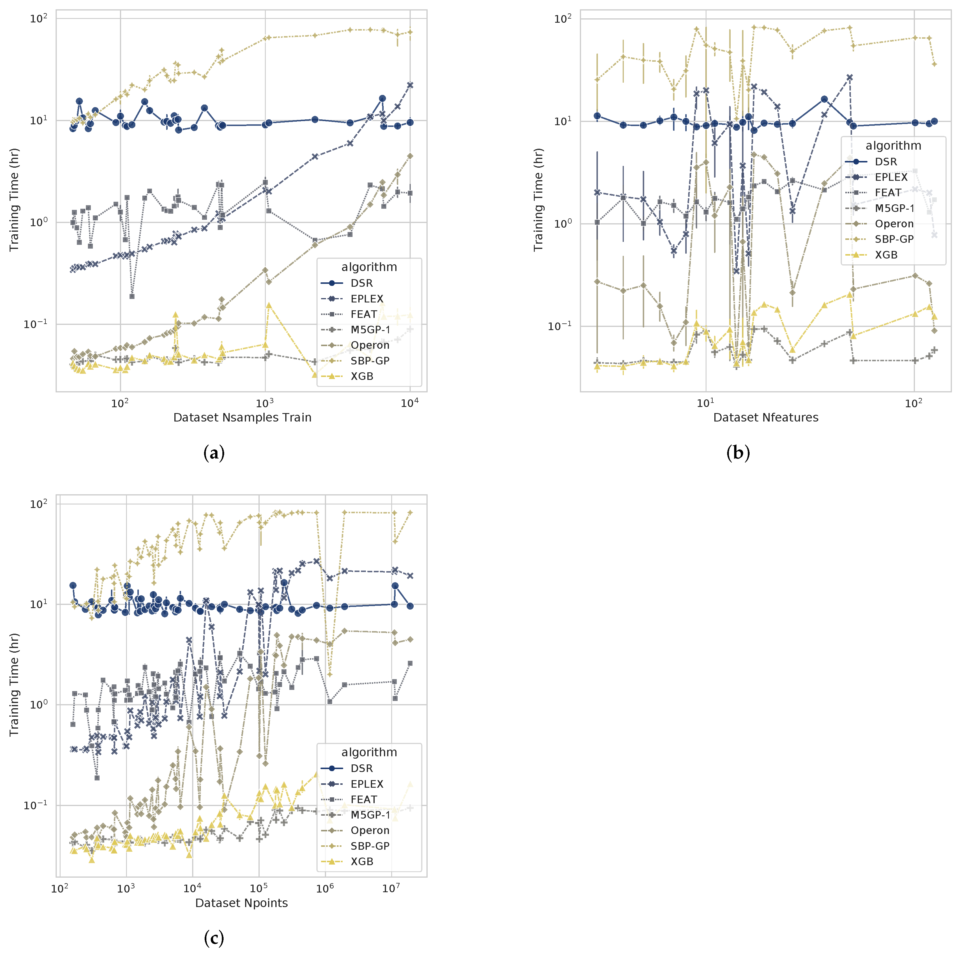
4.3. Computational Cost

Figure 10 summarizes the runtime performance of the best-performing methods and those that are explicitly focused on producing human-readable models. The plots consider the number of training samples, the total number of problem features and a combination of both quantities. The performance of M5GP-1 is similar to that of XGB, clearly outperforming all other methods. What is important is that both factors, the number of training samples ($Nsamples$) and the number of features ($Nfeatures$), have little impact on runtime. Similarly, considering $Npoints=Nsamples\times Nfeatures$ as a measure of the total size of the learning problems, it is clear that M5GP-1 outperforms all other methods except for XGB.

To further evaluate the efficiency of the M5GP implementation, a speed evaluation was performed similarly to the work presented in [7]. GP operations per second (GPops/second) are measured during a full evolutionary run on a problem with 1000 fitness cases and 25 features. The algorithm was executed for 30 generations using a population of 256 individuals and an individual size of 128 genes. With this configuration, M5GP reaches $1.49\times {10}^8$ GPops/second, on average. It is important to mention, however, that the GPops was not used to measur the effort required by the parameter estimation process done by cuML, an integral part of the M5GP modelling process, making direct comparisons with previous works less straightforward [42,43]. Nonetheless, it is important to mention that state-the-art GPU-based implementations of GP, such as those in [42,43], have been shown to reach very high GPops. However, these methods implement a standard GP-based search, similar to the one used by GPlearn, making it reasonable to assume that their performance on SRBench, based on accuracy, would also be similar to that method.

5. Conclusions and Future Work

This paper presents M5GP, a GPU-based feature transformation method that is combined with multiple linear regression to perform constrained SR. The method is based on the previously proposed M2GP, M3GP and M4GP family of feature transformation methods. It utilizes an efficient GPU-based implementation in Python using Numba, using GP search as the feature transformation method and hybridizing with cuML for parameter estimation of a linear model. Results show that the proposed method can achieve state-of-the-art SR results with highly competitive performance relative to other contemporary approaches. Since it employs a powerful machine learning library, cuML, it can potentially be expanded and hybridized with a variety of other approaches, even if our current results show that best performance is achieved using standard LR for parameter estimation. The proposed GPU-based implementation has been shown to be efficient, particularly relative to other GP methods for SR. It even outperformed Operon, the most efficient CPU-based approach. This is a notable result, since Operon is the most accurate method in SRBench and has been shown to be more efficient than previous GPU-based implementations of GP [49]. Indeed, performance on the SRBench benchmark suite shows that runtimes are largely robust to the size of the learning problem. This is an important takeaway from this work: GP-based SR methods need to be designed and implemented with the goal of exploiting the computing advantages provided by modern GPUs.

Future work will focus on combining M5GP with other machine learning algorithms, for dimensionality reduction and/or for classification tasks, the original application domain of M2GP and M3GP. Furthermore, other selection strategies and variation operators can be tested, along with an expanded function set. Moreover, a goal is to integrate a fitness measure that explicitly takes into account the possible interpretability of the evolved solutions. However, care should be taken, as increased sophistication adds also layers of complexity that may limit the usefulness of the approach in a real-world setting. Hyperparameter tuning of M5GP should also be expanded, to configure the cuML methods used to estimate the parameters of the linear models, particularly for the regularized regression methods that did not perform well in these tests. Comparisons with methods not currently included in SRBench should also be performed, using different problems and performance criteria, considering, for example, previous iterations of the M5GP approach [9,23] or more recent methods based on different formulations of the SR problem [64,65,66]. Finally, the main bottleneck of the current implementation is the reliance on cuML, which does not allow for an efficient estimation process for multiple models concurrently, and, therefore, population evaluation is sequential, even though it is independent for each individual and could be done using either a parallel or distributed computation. Therefore, future work will employ alternative approaches and tools to perform parameter estimation of the M5GP models. Nonetheless, for now, it is clear that M5GP should be considered as a state-of-the-art approach for the difficult learning problem of automatically generating symbolic models for a set of training data.

References

1. Koza, J.R. Genetic Programming; Complex Adaptive Systems, Bradford Books: Cambridge, MA, USA, 1992. [Google Scholar]
2. Koza, J.R. Human-competitive results produced by genetic programming. Genet. Program. Evolvable Mach. 2010, 11, 251–284. [Google Scholar] [CrossRef]
3. Orzechowski, P.; La Cava, W.; Moore, J.H. Where Are We Now? A Large Benchmark Study of Recent Symbolic Regression Methods. In Proceedings of the GECCO ’18: Genetic and Evolutionary Computation Conference, Kyoto, Japan, 15–19 July 2018; Association for Computing Machinery: New York, NY, USA, 2018; pp. 1183–1190. [Google Scholar]
4. La Cava, W.; Orzechowski, P.; Burlacu, B.; de Franca, F.; Virgolin, M.; Jin, Y.; Kommenda, M.; Moore, J. Contemporary Symbolic Regression Methods and Their Relative Performance. arXiv 2021, arXiv:2107.14351. [Google Scholar]
5. Rudin, C. Stop explaining black box machine learning models for high stakes decisions and use interpretable models instead. Nat. Mach. Intell. 2019, 1, 206–215. [Google Scholar] [CrossRef] [PubMed]
6. Spector, L.; Robinson, A. Genetic Programming and Autoconstructive Evolution with the Push Programming Language. Genet. Program. Evolvable Mach. 2002, 3, 7–40. [Google Scholar] [CrossRef]
7. Burlacu, B.; Kronberger, G.; Kommenda, M. Operon C++: An Efficient Genetic Programming Framework for Symbolic Regression. In Proceedings of the GECCO ’20: 2020 Genetic and Evolutionary Computation Conference Companion, Cancún, Mexico, 8–12 July 2020; Association for Computing Machinery: New York, NY, USA, 2020; pp. 1562–1570. [Google Scholar]
8. Arnaldo, I.; Krawiec, K.; O’Reilly, U.M. Multiple Regression Genetic Programming. In Proceedings of the GECCO ’14: 2014 Annual Conference on Genetic and Evolutionary Computation, Vancouver, BC, Canada, 12–16 July 2014; Association for Computing Machinery: New York, NY, USA, 2014; pp. 879–886. [Google Scholar]
9. Muñoz, L.; Silva, S.; Trujillo, L. M3GP—Multiclass Classification with GP. In Lecture Notes in Computer Science; Springer International Publishing: Berlin/Heidelberg, Germany, 2015; pp. 78–91. [Google Scholar]
10. Moraglio, A.; Krawiec, K.; Johnson, C.G. Geometric Semantic Genetic Programming. In Proceedings of the PPSN’12: 12th International Conference on Parallel Problem Solving from Nature—Volume Part I, Taormina, Italy, 1–5 September 2012; pp. 21–31. [Google Scholar]
11. Muñoz, L.; Trujillo, L.; Silva, S. Transfer learning in constructive induction with Genetic Programming. Genet. Program. Evolvable Mach. 2019, 21, 529–569. [Google Scholar] [CrossRef]
12. Montgomery, D.C.; Peck, E.A.; Vining, G.G. Introduction to Linear Regression Analysis, 6th ed.; Wiley Series in Probability and Statistics; John Wiley & Sons: Nashville, TN, USA, 2021. [Google Scholar]
13. Rudin, C. Do Simpler Models Exist and How Can We Find Them? In Proceedings of the KDD ’19: 25th ACM SIGKDD International Conference on Knowledge Discovery and Data Mining, Anchorage, AK, USA, 4–8 August 2019; pp. 1–2. [Google Scholar]
14. Tian, Y.; Zhang, Y. A comprehensive survey on regularization strategies in machine learning. Inf. Fusion 2022, 80, 146–166. [Google Scholar] [CrossRef]
15. Trujillo, L.; Z-Flores, E.; Juárez-Smith, P.S.; Legrand, P.; Silva, S.; Castelli, M.; Vanneschi, L.; Schütze, O.; Muñoz, L. Local Search is Underused in Genetic Programming. In Genetic and Evolutionary Computation; Springer International Publishing: Berlin/Heidelberg, Germany, 2018; pp. 119–137. [Google Scholar]
16. Iba, H. Inference of differential equation models by genetic programming. Inf. Sci. 2008, 178, 4453–4468. [Google Scholar] [CrossRef]
17. Pan, I.; Das, S. When Darwin meets Lorenz: Evolving new chaotic attractors through genetic programming. Chaos Solitons Fractals 2015, 76, 141–155. [Google Scholar] [CrossRef]
18. Falco, I.; Cioppa, A.; Tarantino, E. A Genetic Programming System for Time Series Prediction and Its Application to El Niño Forecast. In Advances in Soft Computing; Springer-Verlag: Berlin/Heidelberg, Germany, 1999; pp. 151–162. [Google Scholar]
19. Arfken, G.B.; Weber, H.J.; Harris, F.E. Mathematical Methods for Physicists, 6th ed.; Academic Press: San Diego, CA, USA, 2005. [Google Scholar]
20. McConaghy, T. FFX: Fast, Scalable, Deterministic Symbolic Regression Technology. In Genetic and Evolutionary Computation; Springer: New York, NY, USA, 2011; pp. 235–260. [Google Scholar]
21. Cranmer, M. Interpretable Machine Learning for Science with PySR and SymbolicRegression.jl. arXiv 2023, arXiv:2305.01582. [Google Scholar]
22. Ingalalli, V.; Silva, S.; Castelli, M.; Vanneschi, L. A Multi-dimensional Genetic Programming Approach for Multi-class Classification Problems. In Lecture Notes in Computer Science; Springer: Berlin/Heidelberg, Germany, 2014; pp. 48–60. [Google Scholar]
23. Cava, W.L.; Silva, S.; Danai, K.; Spector, L.; Vanneschi, L.; Moore, J.H. Multidimensional genetic programming for multiclass classification. Swarm Evol. Comput. 2019, 44, 260–272. [Google Scholar] [CrossRef]
24. Muñoz, L.; Trujillo, L.; Silva, S.; Castelli, M.; Vanneschi, L. Evolving multidimensional transformations for symbolic regression with M3GP. Memetic Comput. 2018, 11, 111–126. [Google Scholar] [CrossRef]
25. Helmuth, T.; McPhee, N.F.; Spector, L. Program Synthesis Using Uniform Mutation by Addition and Deletion. In Proceedings of the GECCO ’18: Genetic and Evolutionary Computation Conference, Kyoto, Japan, 15–19 July 2018; Association for Computing Machinery: New York, NY, USA, 2018; pp. 1127–1134. [Google Scholar]
26. Trujillo, L.; Muñoz Contreras, J.M.; Hernandez, D.E.; Castelli, M.; Tapia, J.J. GSGP-CUDA—A CUDA framework for Geometric Semantic Genetic Programming. SoftwareX 2022, 18, 101085. [Google Scholar] [CrossRef]
27. Raschka, S.; Patterson, J.; Nolet, C. Machine learning in Python: Main developments and technology trends in data science, machine learning, and artificial intelligence. Information 2020, 11, 193. [Google Scholar] [CrossRef]
28. Buitinck, L.; Louppe, G.; Blondel, M.; Pedregosa, F.; Mueller, A.; Grisel, O.; Niculae, V.; Prettenhofer, P.; Gramfort, A.; Grobler, J.; et al. API design for machine learning software: Experiences from the scikit-learn project. arXiv 2013, arXiv:1309.0238. [Google Scholar]
29. Chandrashekar, G.; Sahin, F. A Survey on Feature Selection Methods. Comput. Electr. Eng. 2014, 40, 16–28. [Google Scholar] [CrossRef]
30. Cava, W.L.; Singh, T.R.; Taggart, J.; Suri, S.; Moore, J.H. Learning Concise Representations for Regression by Evolving Networks of Trees. arXiv 2019, arXiv:1807.00981. [Google Scholar]
31. Altarabichi, M.G.; Nowaczyk, S.; Pashami, S.; Mashhadi, P.S. Fast Genetic Algorithm for feature selection—A qualitative approximation approach. Expert Syst. Appl. 2023, 211, 118528. [Google Scholar] [CrossRef]
32. Liao, L.; Pindur, A.K.; Iba, H. Genetic Programming with Random Binary Decomposition for Multi-Class Classification Problems. In Proceedings of the 2021 IEEE Congress on Evolutionary Computation (CEC), Krakow, Poland, 28 June–1 July 2021; IEEE: New York, NY, USA, 2021. [Google Scholar]
33. Viegas, F.; Rocha, L.; Gonçalves, M.; Mourão, F.; Sá, G.; Salles, T.; Andrade, G.; Sandin, I. A Genetic Programming approach for feature selection in highly dimensional skewed data. Neurocomputing 2018, 273, 554–569. [Google Scholar] [CrossRef]
34. Espejo, P.; Ventura, S.; Herrera, F. A Survey on the Application of Genetic Programming to Classification. IEEE Trans. Syst. Man Cybern. C Appl. Rev. 2010, 40, 121–144. [Google Scholar] [CrossRef]
35. Z-Flores, E.; Trujillo, L.; Schütze, O.; Legrand, P. A Local Search Approach to Genetic Programming for Binary Classification. In Proceedings of the GECCO ’15: 2015 Annual Conference on Genetic and Evolutionary Computation, Madrid, Spain, 11–15 July 2015; Association for Computing Machinery: New York, NY, USA, 2015; pp. 1151–1158. [Google Scholar]
36. Langdon, W.B. Failed Disruption Propagation in Integer Genetic Programming. In Proceedings of the GECCO ’22: Genetic and Evolutionary Computation Conference Companion, Boston, MA, USA, 9–13 July 2022; Association for Computing Machinery: New York, NY, USA, 2022; pp. 574–577. [Google Scholar]
37. Batista, J.E.; Silva, S. Comparative study of classifier performance using automatic feature construction by M3GP. In Proceedings of the 2022 IEEE Congress on Evolutionary Computation (CEC), Padua, Italiy, 18–23 July 2022; IEEE: New York, NY, USA, 2022. [Google Scholar]
38. Chen, T.; Guestrin, C. XGBoost: A Scalable Tree Boosting System. In Proceedings of the KDD ’16: 22nd ACM SIGKDD International Conference on Knowledge Discovery and Data Mining, San Francisco, CA, USA, 13–17 August 2016; Association for Computing Machinery: New York, NY, USA, 2016; pp. 785–794. [Google Scholar]
39. Batista, J.E.; Cabral, A.I.R.; Vasconcelos, M.J.P.; Vanneschi, L.; Silva, S. Improving Land Cover Classification Using Genetic Programming for Feature Construction. Remote Sens. 2021, 13, 1623. [Google Scholar] [CrossRef]
40. Yang, Y.; Wang, X.; Zhao, X.; Huang, M.; Zhu, Q. M3GPSpectra: A novel approach integrating variable selection/construction and MLR modeling for quantitative spectral analysis. Anal. Chim. Acta 2021, 1160, 338453. [Google Scholar] [CrossRef] [PubMed]
41. Zhou, Z.; Yang, Y.; Zhang, G.; Xu, L.; Wang, M. EBM3GP: A novel evolutionary bi-objective genetic programming for dimensionality reduction in classification of hyperspectral data. Infrared Phys. Technol. 2023, 129, 104577. [Google Scholar] [CrossRef]
42. Langdon, W.B. Graphics processing units and genetic programming: An overview. Soft Comput. 2011, 15, 1657–1669. [Google Scholar] [CrossRef]
43. Chitty, D.M. Faster GPU-based genetic programming using a two-dimensional stack. Soft Comput. 2016, 21, 3859–3878. [Google Scholar] [CrossRef]
44. Spector, L. Assessment of Problem Modality by Differential Performance of Lexicase Selection in Genetic Programming: A Preliminary Report. In Proceedings of the GECCO ’12: 14th Annual Conference Companion on Genetic and Evolutionary Computation, Philadelphia, PA, USA, 7– 11 July 2012; Association for Computing Machinery: New York, NY, USA, 2012; pp. 401–408. [Google Scholar]
45. Schmidt, M.D.; Lipson, H. Age-Fitness Pareto Optimization. In Proceedings of the GECCO ’10: 12th Annual Conference on Genetic and Evolutionary Computation, Cancun, Mexico, 8–12 July 2020; Association for Computing Machinery: New York, NY, USA, 2010; pp. 543–544. [Google Scholar]
46. Olson, R.S.; Bartley, N.; Urbanowicz, R.J.; Moore, J.H. Evaluation of a Tree-based Pipeline Optimization Tool for Automating Data Science. In Proceedings of the GECCO ’16: Genetic and Evolutionary Computation Conference 2016, Denver, CO, USA, 20–24 July 2016; Association for Computing Machinery: New York, NY, USA, 2016; pp. 485–492. [Google Scholar]
47. McDermott, J.; White, D.R.; Luke, S.; Manzoni, L.; Castelli, M.; Vanneschi, L.; Jaskowski, W.; Krawiec, K.; Harper, R.; De Jong, K.; et al. Genetic Programming Needs Better Benchmarks. In Proceedings of the GECCO ’12: 14th Annual Conference on Genetic and Evolutionary Computation, Philadelphia, PA, USA, 7–11 July 2012; Association for Computing Machinery: New York, NY, USA, 2012; pp. 791–798. [Google Scholar]
48. McDermott, J.; Kronberger, G.; Orzechowski, P.; Vanneschi, L.; Manzoni, L.; Kalkreuth, R.; Castelli, M. Genetic Programming Benchmarks: Looking Back and Looking Forward. SIGEVOlution 2022, 15, 1–19. [Google Scholar] [CrossRef]
49. Crary, C.; Piard, W.; Stitt, G.; Bean, C.; Hicks, B. Using FPGA Devices to Accelerate Tree-Based Genetic Programming: A Preliminary Exploration with Recent Technologies. In Lecture Notes in Computer Science; Springer Nature: Cham, Switzerland, 2023; pp. 182–197. [Google Scholar]
50. Virgolin, M.; Alderliesten, T.; Bosman, P.A.N. Linear Scaling with and within Semantic Backpropagation-Based Genetic Programming for Symbolic Regression. In Proceedings of the GECCO ’19: Genetic and Evolutionary Computation Conference, Prague, Czech Republic, 13–17 July 2019; Association for Computing Machinery: New York, NY, USA; pp. 1084–1092. [Google Scholar]
51. Melo, V.V.D. Kaizen programming. In Proceedings of the 2014 Annual Conference on Genetic and Evolutionary Computation, Vancouver, BC, Canada, 12–16 July 2014; ACM: New York, NY, USA, 2014. [Google Scholar]
52. de Franca, F.O.; Aldeia, G.S.I. Interaction–Transformation Evolutionary Algorithm for Symbolic Regression. Evol. Comput. 2021, 29, 367–390. [Google Scholar] [CrossRef] [PubMed]
53. Lam, S.K.; Pitrou, A.; Seibert, S. Numba: A llvm-based python jit compiler. In Proceedings of the Second Workshop on the LLVM Compiler Infrastructure in HPC, Austin, TX, USA, 15 November 2015; pp. 1–6. [Google Scholar]
54. Ni, J.; Drieberg, R.H.; Rockett, P.I. The Use of an Analytic Quotient Operator in Genetic Programming. IEEE Trans. Evol. Comput. 2012, 17, 146–152. [Google Scholar] [CrossRef]
55. Okuta, R.; Unno, Y.; Nishino, D.; Hido, S.; Loomis, C. CuPy: A NumPy-Compatible Library for NVIDIA GPU Calculations. In Proceedings of the 31st Conference on Neural Information Processing Systems (NIPS 2017), Long Beach, CA, USA, 4–9 December 2017. [Google Scholar]
56. Olson, R.S.; La Cava, W.; Orzechowski, P.; Urbanowicz, R.J.; Moore, J.H. PMLB: A large benchmark suite for machine learning evaluation and comparison. BioData Min. 2017, 10, 36. [Google Scholar] [CrossRef]
57. Schapire, R.E. Explaining adaboost. In Empirical Inference; Springer: Berlin/Heidelberg, Germany, 2013; pp. 37–52. [Google Scholar]
58. Ho, T.K. Random decision forests. In Proceedings of the 3rd International Conference on Document Analysis and Recognition, Montreal, QC, Canada, 14–15 August 1995; IEEE: New York, NY, USA, 1995; Volume 1, pp. 278–282. [Google Scholar]
59. Virgolin, M.; Alderliesten, T.; Witteveen, C.; Bosman, P.A.N. Scalable Genetic Programming by Gene-Pool Optimal Mixing and Input-Space Entropy-Based Building-Block Learning. In Proceedings of the GECCO ’17: Genetic and Evolutionary Computation Conference, Berlin, Germany, 15–19 July 2017; Association for Computing Machinery: New York, NY, USA, 2017; pp. 1041–1048. [Google Scholar]
60. Petersen, B.K.; Landajuela, M.; Mundhenk, T.N.; Santiago, C.P.; Kim, S.K.; Kim, J.T. Deep symbolic regression: Recovering mathematical expressions from data via risk-seeking policy gradients. In Proceedings of the International Conference on Learning Representations, Virtual Only Conference, 3–7 May 2021. [Google Scholar]
61. Sipper, M.; Fu, W.; Ahuja, K.; Moore, J.H. Investigating the parameter space of evolutionary algorithms. BioData Min. 2018, 11, 2. [Google Scholar] [CrossRef]
62. Trujillo, L.; Álvarez González, E.; Galván, E.; Tapia, J.J.; Ponsich, A. On the Analysis of Hyper-Parameter Space for a Genetic Programming System with Iterated F-Race. Soft Comput. 2020, 24, 14757–14770. [Google Scholar] [CrossRef]
63. Brookhouse, J.; Otero, F.E.; Kampouridis, M. Working with OpenCL to Speed up a Genetic Programming Financial Forecasting Algorithm: Initial Results. In Proceedings of the GECCO Comp’14: Companion Publication of the 2014 Annual Conference on Genetic and Evolutionary Computation, Vancouver, BC, Canada, 12–16 July 2014; Association for Computing Machinery: New York, NY, USA, 2014; pp. 1117–1124. [Google Scholar]
64. Kamienny, P.-A.; d’Ascoli, S.; Lample, G.; Charton, F. End-to-end Symbolic Regression with Transformers. In Advances in Neural Information Processing Systems; Koyejo, S., Mohamed, S., Agarwal, A., Belgrave, D., Cho, K., Oh, A., Eds.; Curran Associates, Inc.: New York, NY, USA, 2022; Volume 35, pp. 10269–10281. [Google Scholar]
65. Zhang, R.; Lensen, A.; Sun, Y. Speeding up Genetic Programming Based Symbolic Regression Using GPUs. In Proceedings of the PRICAI 2022: Trends in Artificial Intelligence, Shanghai, China, 10–13 November 2022; Khanna, S., Cao, J., Bai, Q., Xu, G., Eds.; Springer Nature: Cham, Switzerland, 2022; pp. 519–533. [Google Scholar]
66. Holt, S.; Qian, Z.; van der Schaar, M. Deep Generative Symbolic Regression. In Proceedings of the The Eleventh International Conference on Learning Representations, Kigali, Rwanda, 1–5 May 2023. [Google Scholar]
Figure 1. Wrapper-based processing for feature transformation with GP.
Mca 29 00025 g001
Figure 2. A set of individuals generated randomly in M5GP, each one on a single GPU thread using a Numba kernel.
Mca 29 00025 g002
Figure 3. Interpreter and stack-based processing in M5GP based on [23] of the first individual in Figure 2. The variable values used in the example are: X 1 = 2 , X 2 = 7 , X 3 = 1, X 4 = 3 and X 5 = 4 .
Mca 29 00025 g003
Figure 4. Parallel processing of the training data to generate the semantic matrix of each individual transformation model.
Mca 29 00025 g004
Figure 5. SRBench performance on the black-box regression problems for all M5GP variants in Table 1: (a) R 2 test set performance, (b) model size (functions and terminals in the model), and (c) total runtime during training. (*) Represents the method returns a symbolic model.
Mca 29 00025 g005
Figure 6. SRBench performance of M5GP compared to other methods, considering configuration M5GP-1, M5GP-2, M5GP-3 and M5GP-4: (a) R 2 test set performance, (b) model size (terms and operators in the model), and (c) total runtime during training. (*) Represents the method returns a symbolic model.
Mca 29 00025 g006
Figure 7. Wilcoxon signed-rank test comparisons from SRBench considering M5GP-1. (a) R 2 . (b) Model size.
Mca 29 00025 g007
Figure 8. Performance of M5GP on the black-box problems, showing improved performance on the Friedman subset of problems.
Mca 29 00025 g008
Figure 9. SRBench performance of M5GP on the ground-truth problems: (a) accuracy based on R 2 and (b) solution rate given in percentage. Results are shown for both datasets used, Feynman and Strogatz.
Mca 29 00025 g009
Figure 10. Training time relative to: (a) the number of samples ( N s a m p l e s ) used during training (b), the number of features ( N f e a t u r e s ); and (c) the total size of the problem ( N p o i n t s = N s a m p l e s × N f e a t u r e s ).
Mca 29 00025 g010