Article

Robust qLPV Tracking Fault-Tolerant Control of a 3 DOF Mechanical Crane

by
Francisco-Ronay López-Estrada
1,
Oscar Santos-Estudillo
1,
Guillermo Valencia-Palomo
2,*,
Samuel Gómez-Peñate
1 and
Carlos Hernández-Gutiérrez
1
1
TURIX-Dynamics Diagnosis and Control Group, Tecnológico Nacional de México, IT Tuxtla Gutiérrez, Carretera Panamericana Km 1080, C.P. 29050 Tuxtla Gutiérrez, Chiapas, Mexico
2
Tecnológico Nacional de México, IT Hermosillo, Ave. Tecnológico y Periférico Poniente S/N, C.P. 83170 Hermosillo, Sonora, Mexico
*
Author to whom correspondence should be addressed.
Math. Comput. Appl. 2020, 25(3), 48; https://doi.org/10.3390/mca25030048
Submission received: 5 July 2020 / Revised: 21 July 2020 / Accepted: 28 July 2020 / Published: 28 July 2020

Abstract

:
The main aim of this paper is to propose a robust fault-tolerant control for a three degree of freedom (DOF) mechanical crane by using a convex quasi-Linear Parameter Varying (qLPV) approach for modeling the crane and a passive fault-tolerant scheme. The control objective is to minimize the load oscillations while the desired path is tracked. The convex qLPV model is obtained by considering the nonlinear sector approach, which can represent exactly the nonlinear system under the bounded nonlinear terms. To improve the system safety, tolerance to partial actuator faults is considered. Performance requirements of the tracking control system are specified in an H criteria that guarantees robustness against measurement noise, and partial faults. As a result, a set of Linear Matrix Inequalities is derived to compute the controller gains. Numerical experiments on a realistic 3 DOF crane model confirm the applicability of the control scheme.

1. Introduction

In recent years, fault-tolerant control (FTC) has become a relevant research field and has attracted significant attention because of its applicability to industrial systems, which increases their security and reliability. A fault can be defined as abnormal behavior of at least one characteristic property or parameter that changes the system performance [1,2]. It is important to note that a fault denotes a breakdown rather than a catastrophe [3,4]. In other words, a fault not necessarily ends in a system stop. However, if no action is taken on time, the system performance begins to degrade that could end in a catastrophe [5]. Therefore, in order to guarantee a minimum level of performance, it is necessary to develop methods to improve system safety and reliability.
Model-based safety schemes require differential equations representing the complex dynamics presented in physical systems, which are often nonlinear [6,7]. Recently, multimodel techniques such as Linear Parameter Varying (LPV), quasi-LPV (qLPV), and Takagi–Sugeno (TS) systems have emerged as an attractive alternative to deal with the analysis of complex nonlinear systems due to the fact that it is possible to extend techniques developed for linear systems but applied to nonlinear systems [8,9,10,11]. In this paper, it is considered that qLPV and TS systems are the same because the convex model is obtained through the so-called nonlinear sector approach [12]. This paradigm has been extensively studied in the works of [13,14]. In the literature, FTC systems have been classified into two approaches: passive and active [15]. Passive FTC is an extension of robust control [16] and requires some knowledge of possible failures that may affect the system. In this scheme, the controller is designed a priori to be robust to faults, and non-online adaptation is made. This type of control is interesting because it does not need any fault diagnosis module [17]. In contrast, active FTC systems offer flexibility in the design task. They are assimilated as a variable structure technique because the controller is reconfigured when a fault occurs [18]. However, it is necessary to include a Fault Diagnosis and Isolation (FDI) module, which provides information about the faults [19,20]. The inclusion of the FDI module gives some conservatism into the controller solution. This work is dedicated to the study of passive fault-tolerant with application to a mechanical crane.
A mechanical crane can load hundreds of tons and are widely used in oil platforms, ships, factories, railway depots, piers, among others [21]. By design, the crane is a sub-actuated system, which means that it has more degrees of freedom (DOF) than control inputs. In the particular case of the crane shown in Figure 1, it is assumed that the load is attached to a plane. The degrees of freedom of the crane are three: the first one refers to movement on the x-axis (forward/backward movement of the carriage); the second on the z-axis (up/down movement of the load); and finally the angular displacement of the load on the x-axis. However, the system has only two actuators, which are the trolley motor and the hoist motor. The control objective is to locate the crane at the desired position, whereby the trolley motor moves the load as fast as possible. At the same time, the oscillations that could destabilize the system must be minimized [22]. Due to this, it is essential to design control schemes that consider the under-actuation, a large number of linearities, possible faults, and robustness to the payload oscillations.
In the literature, this problem has been approached by considering different methods, e.g., sliding modes [23], LQ controllers [24], particle swarm optimization [25], adaptive control [26,27], among others. Regarding safety systems, sliding mode differentiators can be consulted in [28] and fault-tolerant control in [29,30]. Some authors have explored the design of robust controllers based on multimodel techniques. For example, in [31], a robust stabilization method based on TS models was proposed. The authors in [32] presented a hybrid controller that includes position regulation and oscillation control designed using TS techniques. Similarly, in [33], a reduced-order H 2 / H LPV controller was proposed. In [34] a distributed parallel compensation control is explored through TS techniques. In [35], a fault-tolerant LPV control was proposed. Authors in [36] proposed a reconfiguration scheme for active fault tolerance by considering predictive control. However, none of the reported works were subjected to performance tests in the presence of disturbances by unknown additive signals.
This paper is devoted to developing a robust quasi-Linear Parameter Varying (qLPV) fault tolerant-control system with H criteria applied to a 3 DOF crane. The main idea is to propose a control law that minimize oscillations in the load while the desired path is tracked. The proposed method is robust to disturbances, sensor noise, and partial faults. The method performance and applicability are tested through numerical simulations on a 3 DOF mechanical crane by compensating partial faults on the trolley and load motors.

2. Mathematical Modeling

The free-body diagram of three degrees of freedom traveling crane is shown in Figure 1. The cart slides along a horizontal rail and at the same time that it is supported by two metal legs. A mass is suspended from a cable attached to the cart. Force F x is applied to the cart, which provokes a displacement in the x-axis. This movement causes an angular displacement θ formed in the pendulum by the load mass m and the cable of length l whose value can be changed by F l , i.e., F l activates the elevation system by means of a motor and gears. The nonlinear model is given by the following ordinary differential equations [23]:
M ( q ) q ¨ + D q ˙ + C ( q , q ˙ ) q ˙ + G ( q ) = F ;
with:
q = x c ( t ) l ( t ) θ ( t ) ; F = F x ( t ) F l ( t ) 0 ; M ( q ) = ( M x + m ) m sin θ ( t ) m l ( t ) cos θ ( t ) m sin θ ( t ) ( M l + m ) 0 m l ( t ) cos θ ( t ) 0 m l ( t ) 2 ;
C ( q , q ˙ ) = 0 2 m cos θ ( t ) θ ˙ ( t ) m l sin θ ( t ) θ ˙ ( t ) 0 0 m l ( t ) θ ˙ ( t ) 0 2 m θ ˙ ( t ) l ( t ) 0 ; D = D x 0 0 0 D l 0 0 0 0 ; G ( q ) = 0 m g m g cos θ ( t ) m g l ( t ) sin θ ( t ) ;
where m is the load mass and g is the gravitational acceleration; D x and D y are the viscous damping coefficients associated with the x- and z-axis respectively; finally, M x and M l are the traveling and hoisting components of the crane mass, respectively, i.e., M x = m + m c and M l = m , where m c is the cart mass. The parameter values considered in this paper are close to a real laboratory crane system, e.g., [37].
The state-space derivation is obtained solving (1) for q ¨ , such as:
q ¨ = M ( q ) 1 D q ˙ M ( q ) 1 C ( q , q ˙ ) q ˙ M ( q ) 1 G ( q ) + M ( q ) 1 F .
By using sin θ ( t ) = S θ , and cos θ ( t ) = C θ ; Equation (2) in long hand becomes,
q ¨ = 0 0 m M l S θ l ( t ) θ ˙ ( t ) μ ( t ) 0 0 m M x l ( t ) θ ˙ ( t ) μ ( t ) 0 2 θ ˙ ( t ) l ( t ) M l m C θ S θ θ ˙ ( t ) μ ( t ) q ˙ ( M l + m ) D x μ ( t ) m S θ D l μ ( t ) 0 m S θ D x μ ( t ) ( M x + m m C θ 2 ) D l μ ( t ) 0 C θ ( M l + m ) D x l ( t ) μ ( t ) m C θ S θ D l l ( t ) μ ( t ) 0 q ˙ m g S θ ( t ) ( M l C θ + m ) μ ( t ) 0 0 ( M x + m + m C θ 2 ) ( m g m g C θ ) + g m 2 C θ S θ 2 μ ( t ) 0 0 0 0 m C θ S θ ( m g m g C θ ) + ( M x M l + M l m + M x m + m 2 m 2 S θ 2 ) g S θ l ( t ) μ ( t )
+ M l + m μ ( t ) m S θ μ ( t ) ( M l + m ) C θ l ( t ) μ ( t ) m S θ μ ( t ) M x + m m C θ 2 μ ( t ) m S θ C θ l ( t ) μ ( t ) ( M l + m ) C θ l ( t ) μ ( t ) m S θ C θ l ( t ) μ ( t ) M l M x + M l m + M x m + m 2 m 2 S θ 2 m ( l ( t ) ) 2 μ ( t ) F x ( t ) F l ( t ) 0 ;
with μ ( t ) = M l M x + M l m + M x m + m 2 M l m C θ 2 m 2 C θ 2 m 2 S θ 2 = M l M x + M l m + M x m M l m C θ 2 . Recalling that q = [ x c ( t ) , l ( t ) , θ ( t ) ] T ; then, by considering small values of θ , i.e., S θ θ , C θ 1 , θ 2 0 , and θ ˙ 2 0 , the following equations can be obtained,
x ¨ c ( t ) = ( M l + m ) D x x ˙ c ( t ) M l M x + M x m + m θ ( t ) D l l ˙ ( t ) M l M x + M x m + ( M l + m ) m g θ ( t ) M l M x + M x m + ( M l + m ) F x ( t ) M l M x + M x m m θ ( t ) F l ( t ) M l M x + M x m ; l ¨ ( t ) = m D x θ ( t ) x ˙ c ( t ) M l M x + M x m M x D l l ˙ ( t ) M l M x + M x m m θ ( t ) F x ( t ) M l M x + M x m + M x F l ( t ) M l M x + M x m ; θ ¨ ( t ) = ( M l + m ) D x x ˙ c ( t ) l ( t ) ( M l M x + M x m ) m D l θ ( t ) l ˙ ( t ) l ( t ) ( M l M x + M x m ) 2 θ ˙ ( t ) l ˙ ( t ) l ( t ) ( M x M l + M l m + M x m + m 2 ) g θ ( t ) l ( t ) ( M l M x + M x m ) ( M l + m ) F x ( t ) l ( t ) ( M l M x + M x m ) + m θ F l ( t ) l ( t ) ( M l M x + M x m ) .
Remark 1.
If θ ( t ) is not assumed to be small, the nonlinear terms would increase, increasing the complexity of the convex system representation resulting in a more involved procedure for the controller design. However, the consideration that the designed controller will keep load oscillations small makes it possible to assume θ 0 .
Finally, by setting x ( t ) = [ x 1 ( t ) , x 2 ( t ) , x 3 ( t ) , x 4 ( t ) , x 5 ( t ) , x 6 ( t ) ] T = [ x c ( t ) , x ˙ c ( t ) , l ( t ) , l ˙ ( t ) , θ ( t ) , θ ˙ ( t ) ] T and u ( t ) = [ F x ( t ) , F l ( t ) ] T , the state space representation is obtained:
x ˙ ( t ) = 0 1 0 0 0 0 0 m 2 D x 0 m 1 D l x 5 m 4 g 0 0 0 0 1 0 0 0 m 1 D x x 5 0 m 3 D l 0 0 0 0 0 0 0 1 0 m 2 D x x 3 0 ( m 1 D l x 5 x 3 + 2 x 6 x 3 ) m 5 g x 3 0 x ( t ) + 0 0 m 2 m 1 x 5 0 0 m 1 x 5 m 3 0 0 m 2 x 3 m 1 x 5 x 3 u ( t ) ;
with m 1 = m / ( M l M x + M x m ) ; m 2 = ( M l + m ) / ( M l M x + M x m ) ; m 3 = M x / ( M l M x + M x m ) ; m 4 = m ( M l + m ) / ( M l M x + M x m ) ; m 5 = ( M x M l + M l m + M x m + m 2 ) / ( M l M x + M x m ) . Note that the nonlinear terms in (4) are given by:
z = x 5 1 x 3 x 5 x 3 x 6 x 3 .
In order to obtain a TS model through the nonlinear sector approach, each nonlinear term is bounded as x 3 [ 0.1 , 0.72 ] [m], x 5 [ 0.35 , 0.35 ] [rad], and x 6 [ 3.467 , 3.467 ] [rad/s], such as the weighting functions are described as:
  • For z 1 = x 5 the limits are z 1 , m i n = 0.35 and z 1 , m a x = 0.35 . The weigthing functions are w 11 = z 1 , m a x z 1 z 1 , m a x z 1 , m i n and w 12 = 1 w 11 . Therefore, z 1 can be rewritten as z 1 = z 1 , m i n w 11 + z 1 , m a x w 12 .
  • For z 2 = 1 x 3 the limits are z 2 , m i n = 1 and z 2 , m a x = 10 . The weighting functions are w 21 = z 2 , m a x z 2 z 2 , m a x z 1 , m i n and w 22 = 1 w 21 . Therefore, z 2 ( t ) can be rewritten as z 2 = z 2 , m i n w 21 + z 2 , m a x w 22 .
  • z 3 = x 5 x 3 is bounded as z 3 , m i n = 3.5 and z 3 , m a x = 3.5 . The weigthing functions are w 31 = z 3 , m a x z 3 z 3 , m a x z 3 , m i n and w 32 = 1 w 31 , with z 3 = z 3 , m i n w 31 + z 3 , m a x w 32 .
  • Finally, z 4 = x 6 x 3 is bounded as z 4 , m i n = 34.67 and z 4 , m a x = 34.67 . The weighting functions are w 41 = z 4 , m a x z 4 z 4 , m a x z 4 , m i n and w 42 = 1 w 41 , with z 4 = z 4 , m i n w 41 + z 4 , m a x w 42 .
Then, the nonlinear model can be represented by:
x ˙ ( t ) = 0 1 0 0 0 0 0 m 2 D x 0 m 1 D l z 1 m 4 g 0 0 0 0 1 0 0 0 m 1 D x z 1 0 m 3 D l 0 0 0 0 0 0 0 1 0 m 2 D x z 2 0 ( m 1 D l z 3 + 2 z 4 ) m 5 g z 2 0 x ( t ) + 0 0 m 2 m 1 z 1 0 0 m 1 z 1 m 3 0 0 m 2 z 2 m 1 z 3 u ( t )
The number of local sub-models is 2 4 = 16 , then, the membership functions are computed as the product of the weighting functions that correspond to each local model,
h i ( z ( t ) ) = j = 1 p w i j j ( z j ) , i = 1 , 2 , , 2 p .
Note that the membership functions are convex which means that h i ( z ( t ) ) 0 , i = 1 16 h i ( z ( t ) ) = 1 . The number of combinations are defined as given in Table 1.
Then, the convex qLPV model is derived as:
x ˙ ( t ) = i = 1 16 h i ( z ) A i x ( t ) + B i u ( t ) ; y ( t ) = C x ( t ) ;
The matrix C is constant as y ( t ) represents the measured output which according to the nature of the system is linear.

3. Convex H Fault-Tolerant Controller

Under the presence of additive actuator faults, system (7) can be rewritten as
x ˙ ( t ) = A h x ( t ) + B h u ( t ) + G h f ( t ) , y ( t ) = C x ( t ) ,
where:
A h = i = 1 16 h i ( z ( x ( t ) ) ) A i , B h = i = 1 16 h i ( z ( x ( t ) ) ) B i ,
f R s represents the additive fault vector and G h R n × s represents the fault matrix. Typically in order to simulate actuator degradation, it is considered that G h = B h .
Then, a convex qLPV controller for the nonlinear 3 DOF crane, as the one shown in Figure 2, is proposed with:
ϵ ˙ ( t ) = ω ( t ) y ( t ) = ω ( t ) C x ( t ) ,
where ω ( t ) is the reference and the control law is defined by:
u ( t ) = i = 1 16 h i ( z ) F 1 i x ( t ) + F 2 i ϵ ( t ) = i = 1 16 h i ( z ) F i x ( t ) ϵ ( t ) = F h x ( t ) ϵ ( t ) ,
where F 1 i and F 2 i are the gain matrices to be computed. Then, the main problem is to determine the optimal values for these control gains, such that the system be robust to disturbances and sensor noise. Then, by considering the tracking comparator in the control scheme (10), the following augmented system is obtained:
x ¯ ˙ ( t ) = A ¯ h x ¯ ( t ) + B ¯ h u ( t ) + G ¯ h f ( t ) + B ¯ ω ω ( t )
with:
A ¯ h = A h 0 C 0 , B ¯ h = B h 0 , B ¯ ω = 0 I , G ¯ h = G h 0 , x ¯ = x ( t ) ϵ ( t ) .
Assuming that the pair [ A ¯ i , B ¯ i ] is controllable and the control law (11), the following closed-loop system is obtained:
x ¯ ˙ = A ¯ h + B ¯ h F h x ¯ + G ¯ h f ( t ) + B ¯ ω ω ( t ) .
System (13) can be rewritten equivalently as:
x ¯ ˙ = A ¯ h + B ¯ h F h x ¯ + G ¯ ω h f ¯ ω ( t ) ,
with:
G ¯ ω h = G ¯ h B ¯ ω , f ¯ ω = f ( t ) ω ( t )
Then, by considering an H performance criteria is considered to design a robust controller F h , which minimizes the energy L 2 -gain of the closed-loop system, such as norm upper bound is simultaneously guaranteed:
x ¯ ( t ) 2 f ¯ ( t ) ω 2 γ , γ > 0 ,
as a result, the following Theorem is derived:
Theorem 1.
Given the qLPV system (7), the robust control (11) has a quadratic γ-performance level if there exist matrices X, M j , with γ > 0 , such that the following optimization problem is solved i , j [ 1 , 2 , , 16 ] :
m i n γ ¯ , s . t .
A ¯ i X + B ¯ i M j + M j T B ¯ i T + X A ¯ i T G ¯ ω i X T G ¯ ω i T γ ¯ I 0 X 0 I 0 .
Then, the controller matrices and the performance are computed by F i = M j X 1 and γ = γ ¯ .
Proof. 
Let us consider the following H performance criteria:
V ˙ ( x ¯ ( t ) ) + x ¯ ( t ) T x ¯ ( t ) γ 2 f ¯ ω ( t ) T f ¯ ω ( t ) ,
where V ˙ ( x ¯ ( t ) ) is the derivative of the quadratic Lyapunov function x ¯ ( t ) T P x ¯ ( t ) > 0 , with P = P T > 0 , over the trajectory of the augmented states, such as the performance criteria can be rewritten as:
x ¯ ˙ ( t ) T P x ¯ ( t ) + x ¯ ( t ) T P x ¯ ˙ ( t ) + x ¯ ( t ) T x ¯ ( t ) γ 2 f ¯ ω ( t ) T f ¯ ω ( t ) 0 .
Then, by considering the augmented matrices given in (14), the following is obtained:
x ¯ T P ( ( A ¯ h + B ¯ h F h ) x ¯ + G ¯ ω h f ¯ ω ) + ( ( A ¯ h + B ¯ h F h ) x ¯ + G ¯ ω h f ¯ ω ) T P x ¯ + x ¯ T x ¯ γ 2 f ¯ ω T f ¯ ω 0 ,
which can be equivalently rewritten as:
x ¯ T ( P A ¯ h + P B ¯ h F h + F h T B ¯ h T P + A ¯ h T P + I ) x ¯ + x ¯ T ( P G ¯ ω h ) f ¯ ω + f ¯ ω T ( G ¯ ω h T P ) x ¯ f ¯ ω T ( γ 2 I ) f ¯ ω 0 .
Then, the performance criteria can be factorized as:
x ¯ T f ¯ ω T P A ¯ h + P B ¯ h F h + F h T B ¯ h T P + A ¯ h T P + I P G ¯ ω h G ¯ ω h T P γ 2 I x ¯ f ¯ ω 0 .
In order to put together the unknown matrices P and F h , the inequality is pre and post-multiplyied by X 0 0 I and its transpose, with X = P 1 , such as the following is obtained:
A ¯ h X + B ¯ h F h X + X F h T B ¯ h T + X A ¯ h T + X T X G ¯ ω h G ¯ ω h T γ 2 I 0
With this transformation, the quadratic term can be eliminated by considering M h = F h X and γ ¯ = γ 2 , such as the following Linear Matrix Inequality (LMI) is derived:
A ¯ h X + B ¯ h M h + M h T B ¯ h T + X A ¯ h T + X T X G ¯ ω h G ¯ ω h T γ ¯ I 0 ,
which can be rewritten as:
A ¯ h X + B ¯ h M h + M h T B ¯ h T + X A ¯ h T G ¯ ω h G ¯ ω h T γ ¯ I + X T 0 I X 0 0 .
Then, by considering the Schur complement, the following LMI is obtained:
A ¯ h X + B ¯ h M h + M h T B ¯ h T + X A ¯ h T G ¯ ω h X T G ¯ ω h T γ ¯ I 0 X 0 I 0 .
Note that (24) and (25) are equivalent, and both can be used to find the gains. However, (25) is written in a relaxed form to reduce the LMI conservatism. Finally, by considering the equivalent matrices in (9), the LMI, as given in Theorem 1, is obtained. This completes the proof. □
Remark 2.
In this paper, the method considers a constant Lyapunov matrix P, which means it is necessary to find a Matrix P such for all 16 LMIs. This problem can be relaxed by considering a parameter-varying P h , which is also called the non-quadratic Lyapunov functions [38]. This problem can reduce the conservatism of the LMI and open new research areas for future work. However, it is essential to understand that powerful semidefinite programming solvers as SEDUMI o Mosek can deal with quadratic functions, as presented in this paper, and it is not necessary to address the non-quadratic problem.

4. Numerical Results

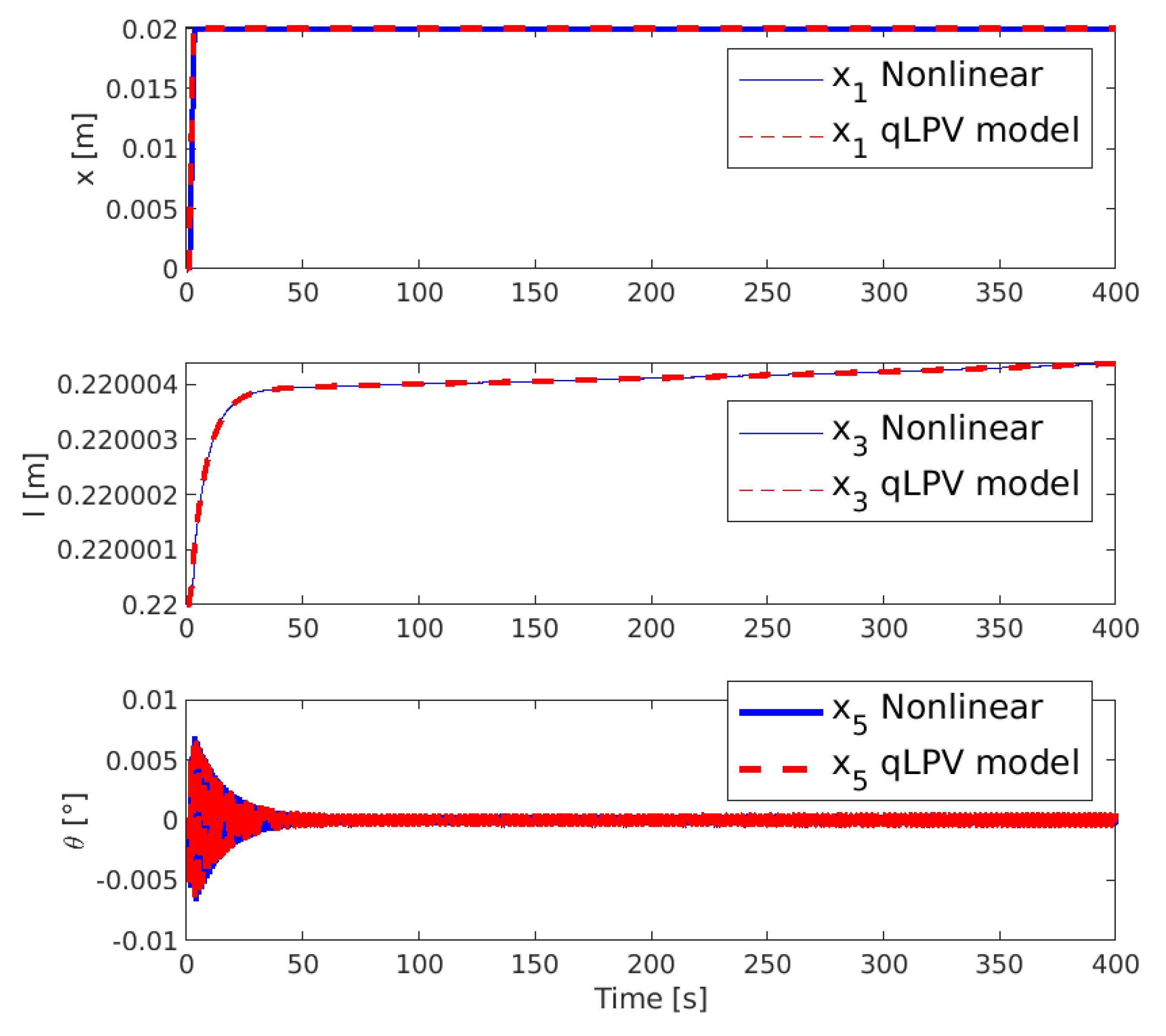
To validate the convex nonlinear model (7) of the 3 DOF crane with respect to the nonlinear model given in [27], the parameters given in Table 2 are considered with initial conditions x ( 0 ) = 0 , l ( 0 ) = 0.22 [m], θ ( 0 ) = 0 . A unit-input pulse it is considered for both actuators from 1 [s] u ( t ) 2 [s], such as the responses shown in Figure 3 are obtained.
For the sake of simplicity and page limitation, only the comparison of the displacements are showed here. As can be observer from Figure 3, the responses of both systems, the nonlinear and the qLPV, are practically the same due to the fact that the convex model represents exactly the nonlinear system on the sectors limited by the weighting functions. Then, this convex model can be used to design the convex controller.
For the controller design, Theorem 1 is solved by minimizing γ such as the LMI (16) is feasible. For such purpose, the YALMIP [39] toolbox and the SEDUMI [40] solver have been used. The computed attenuation level is γ = 0.0314 . Note that an attenuation level γ < 1 guarantees a good robust performance against noise and disturbances. The resulting P matrix is:
P = 29.2989 33.8755 35.2641 25.3974 112.0708 1.1582 33.8755 41.7475 46.7113 29.3192 139.3964 1.8173 35.2641 46.7113 165.1513 2.0182 168.5182 5.5944 25.3974 29.3192 2.0182 87.9937 86.5479 4.0631 112.0708 139.3964 168.5182 86.5479 478.4657 8.7512 1.1582 1.8173 5.5944 4.0631 8.7512 1.4297 .
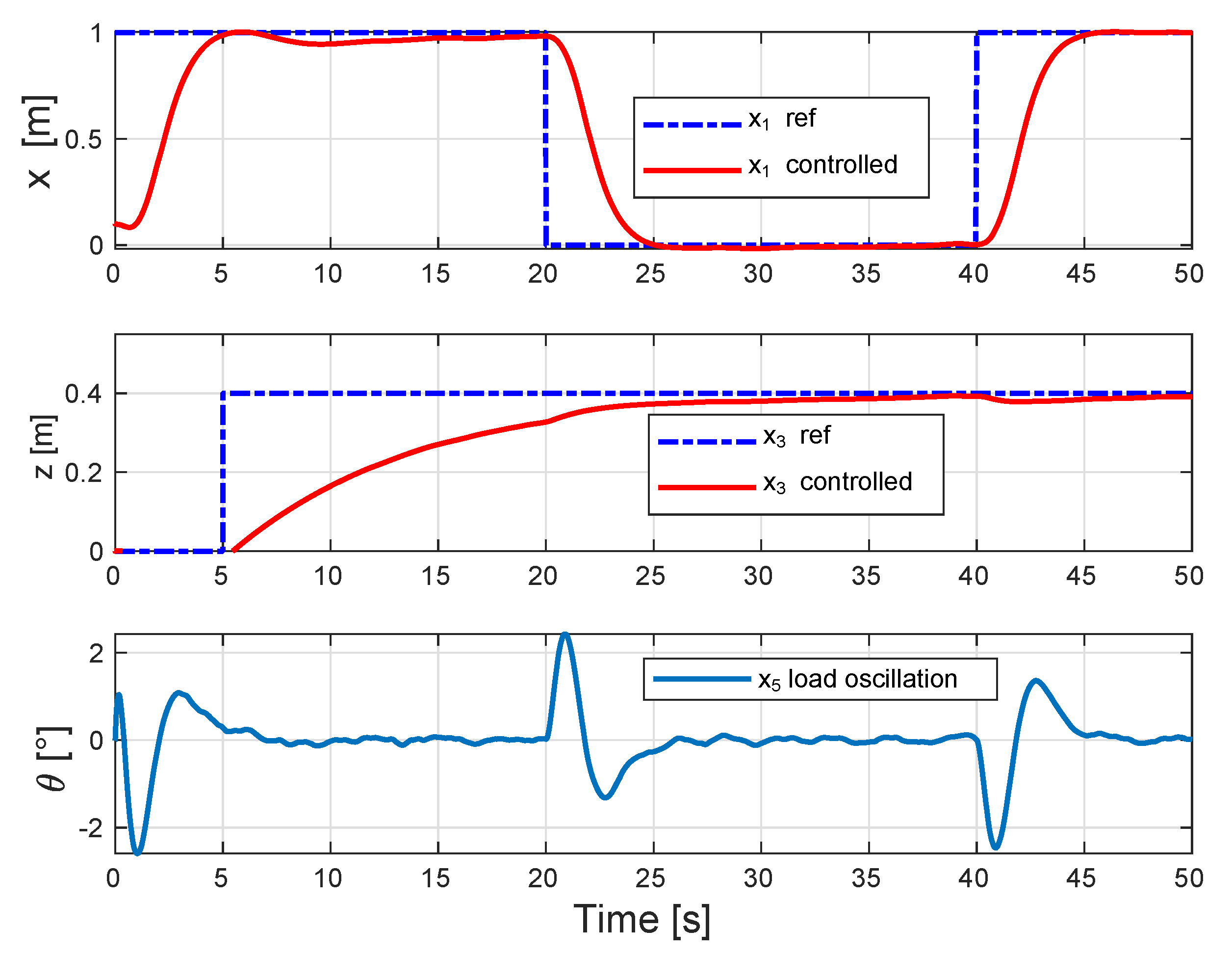
The numerical simulations of the controller were carried-out by considering the initial conditions given earlier and Gaussian random noise with zero mean and variance 0.2 in the measurements. The control objective is to displace the cart to track a reference consisting of a pulse oscillation of 1 [m] from the origin, for 20 [secs] in each position, and maintain the load in 0.4 [m] for t 5 [s]. In addition, in order to evaluate the fault tolerance of the closed-loop system, an additive fault is applied to the input u 1 , the fault is defined as follows:
Fault u 1 = 0 t < 35 15 % of u 1 35 t 45 35 % of u 1 t > 45 .
The fault corresponds to a degradation of the force F x given by the motor of the cart (25% and 35% of its nominal value). To include these faults, the matrix G h = B h , which represents the additive fault. The numerical simulations results are displayed in Figure 4.
As it can be observed, the controller tracks the demanded changes in the cart position and also maintains the load position. As a result that the proposed approach considers a passive fault-tolerant approach, the controller is robust to the actuator’s fault. As it can be analyzed, the fault is compensated as soon as it appears, which means that its effect is practically eliminated from the system response. Different fault scenarios were carried-out to test the controller performance and have been found that for actuator faults involving a degradation higher than 50%, the controller cannot reach the desired tracking position anymore. The effect of the noisy measured signals is reflected in the payload oscillation as this signal looks trembling. In addition, despite the continuous displacement, the load oscillation is attenuated maintaining a maximum of ± 2 degree with respect to the vertical. Nevertheless, this does not represent a limitation because the main objective was to maintain the desired position under partial faults. For more significant faults in magnitude, it would be necessary to replace the motor in order to guarantee the system’s safety.

5. Conclusions

This paper has presented a passive fault-tolerant controller for a 3 degree of freedom mechanical crane. First, a convex model of the 3 DOF crane has been proposed, representing the nonlinear dynamic by a set of linear models interpolated by nonlinear weighting functions. Then, a tracking fault-tolerant controller with H performance criteria has been developed over the nonlinear states’ trajectories. The H performance guarantees robustness against measurement noise and partial faults. The numerical simulations results show the effectivity of the proposed method by tracking a predefined position of the cart and the load while the oscillations are attenuated despite the actuator faults. Future work will investigate the inclusion of measurement noise and will compare the development with a full nonlinear controller such as a nonlinear or sliding model controller.

Author Contributions

Conceptualization, F.-R.L.-E. and S.G.-P.; formal analysis, O.S.-E. and C.H.-G.; methodology, F.-R.L.-E. and G.V.-P.; software O.S.-E. and S.G.-P.; validation G.V.-P. and C.H.-G.; writing—original draft preparation, F.-R.L.-E. and G.V.-P.; writing—review and editing, S.G.-P. and O.S.-E. All authors have read and agreed to the published version of the manuscript.

Funding

The Consejo Estatal de Ciencia y Tecnológia del Estado de Chiapas financed this project under the grant number 1123. Aditional funding was provided from Conacyt, grants Projects 88 and 2759; and Tecnológico Nacional de México, grants 7641.20-P and 8017.20-P.

Conflicts of Interest

The authors declare no conflict of interest. The funders had no role in the design of the study; in the collection, analyses, or interpretation of data; in the writing of the manuscript, or in the decision to publish the results.

References

  1. Blanke, M.; Kinnaert, M.; Lunze, J.; Staroswiecki, M.; Schröder, J. Diagnosis and Fault-Tolerant Control; Springer: Berlin/Heidelberg, Germany, 2006; Volume 691. [Google Scholar]
  2. Martínez-García, C.; Puig, V.; Astorga-Zaragoza, C.M.; Madrigal-Espinosa, G.; Reyes-Reyes, J. Estimation of Actuator and System Faults Via an Unknown Input Interval Observer for Takagi–Sugeno Systems. Processes 2020, 8, 61. [Google Scholar] [CrossRef] [Green Version]
  3. Witczak, M. Fault diagnosis and fault-tolerant control strategies for non-linear systems. Lect. Notes Electr. Eng. 2014, 266, 375–392. [Google Scholar]
  4. García, C.M.; Puig, V.; Astorga-Zaragoza, C.; Osorio-Gordillo, G. Robust fault estimation based on interval takagi–sugeno unknown input observer. IFAC-PapersOnLine 2018, 51, 508–514. [Google Scholar] [CrossRef]
  5. Nagy-Kiss, A.M.; Ichalal, D.; Schutz, G.; Ragot, J. Fault tolerant control for uncertain descriptor multi-models with application to wastewater treatment plant. In Proceedings of the American Control Conference (ACC), Chicago, IL, USA, 1–3 July 2015; pp. 5718–5725. [Google Scholar]
  6. Wu, Y.; Dong, J. Fault detection for T–S fuzzy systems with partly unmeasurable premise variables. Fuzzy Sets Syst. 2018, 338, 136–156. [Google Scholar] [CrossRef]
  7. Quintana, D.; Estrada-Manzo, V.; Bernal, M. Real-time parallel distributed compensation of an inverted pendulum via exact Takagi–Sugeno models. In Proceedings of the 2017 14th International Conference on Electrical Engineering, Computing Science and Automatic Control (CCE), Mexico City, Mexico, 20–22 October 2017; pp. 1–5. [Google Scholar]
  8. López-Estrada, F.R.; Theilliol, D.; Astorga-Zaragoza, C.M.; Ponsart, J.C.; Valencia-Palomo, G.; Camas-Anzueto, J. Fault diagnosis observer for descriptor Takagi–Sugeno systems. Neurocomputing 2019, 331, 10–17. [Google Scholar] [CrossRef]
  9. Gómez-Peñate, S.; López-Estrada, F.R.; Valencia-Palomo, G.; Rotondo, D.; Enríquez-Zárate, J. Actuator and sensor fault estimation based on a proportional-integral quasi-LPV observer with inexact scheduling parameters. IFAC-PapersOnLine 2019, 52, 100–105. [Google Scholar] [CrossRef]
  10. Gómez-Peñate, S.; Valencia-Palomo, G.; López-Estrada, F.R.; Astorga-Zaragoza, C.M.; Osornio-Rios, R.A.; Santos-Ruiz, I. Sensor fault diagnosis based on a sliding mode and unknown input observer for Takagi–Sugeno systems with uncertain premise variables. Asian J. Control 2019, 21, 339–353. [Google Scholar] [CrossRef] [Green Version]
  11. Chen, L.; Alwi, H.; Edwards, C. On the synthesis of an integrated active LPV FTC scheme using sliding modes. Automatica 2019, 110, 108536. [Google Scholar] [CrossRef]
  12. Ohtake, H.; Tanaka, K.; Wang, H.O. Fuzzy modeling via sector nonlinearity concept. Integr. Comput. Aided Eng. 2003, 10, 333–341. [Google Scholar] [CrossRef]
  13. Rotondo, D. Advances in Gain-Scheduling and Fault Tolerant Control Techniques; Springer: Berlin/Heidelberg, Germany, 2017. [Google Scholar]
  14. López-Estrada, F.R.; Rotondo, D.; Valencia-Palomo, G. A Review of Convex Approaches for Control, Observation and Safety of Linear Parameter Varying and Takagi–Sugeno Systems. Processes 2019, 7, 814. [Google Scholar] [CrossRef] [Green Version]
  15. Zhang, Y.; Jiang, J. Bibliographical review on reconfigurable fault-tolerant control systems. Ann. Rev. Control 2008, 32, 229–252. [Google Scholar] [CrossRef]
  16. Yu, X.; Zhang, Y. Design of passive fault-tolerant flight controller against actuator failures. Chin. J. Aeronaut. 2015, 28, 180–190. [Google Scholar] [CrossRef] [Green Version]
  17. Nasiri, A.; Nguang, S.K.; Swain, A.; Almakhles, D. Passive actuator fault tolerant control for a class of MIMO nonlinear systems with uncertainties. Int. J. Control 2019, 92, 693–704. [Google Scholar] [CrossRef]
  18. Liu, Z.; Liu, J.; He, W. Robust adaptive fault tolerant control for a linear cascaded ODE-beam system. Automatica 2018, 98, 42–50. [Google Scholar] [CrossRef]
  19. Nemati, F.; Hamami, S.M.S.; Zemouche, A. A nonlinear observer-based approach to fault detection, isolation and estimation for satellite formation flight application. Automatica 2019, 107, 474–482. [Google Scholar] [CrossRef]
  20. Guzmán-Rabasa, J.A.; López-Estrada, F.R.; González-Contreras, B.M.; Valencia-Palomo, G.; Chadli, M.; Perez-Patricio, M. Actuator fault detection and isolation on a quadrotor unmanned aerial vehicle modeled as a linear parameter-varying system. Meas. Control 2019, 52, 1228–1239. [Google Scholar] [CrossRef] [Green Version]
  21. Kim, Y.S.; Hong, K.S.; Sul, S.K. Anti-sway control of container cranes: Inclinometer, observer, and state feedback. Int. J. Control Autom. Syst. 2004, 2, 435–449. [Google Scholar]
  22. Shi, K.; Wang, B.; Yang, L.; Jian, S.; Bi, J. Takagi–Sugeno fuzzy generalized predictive control for a class of nonlinear systems. Nonlinear Dyn. 2017, 89, 169–177. [Google Scholar] [CrossRef]
  23. Almutairi, N.B.; Zribi, M. Sliding mode control of a three-dimensional overhead crane. J. Vib. Control 2009, 15, 1679–1730. [Google Scholar] [CrossRef]
  24. Castillo, I.; Vázquez, C.; Fridman, L. Overhead crane control through LQ singular surface design MATLAB Toolbox. In Proceedings of the American Control Conference (ACC), Chicago, IL, USA, 1–3 July 2015; pp. 5847–5852. [Google Scholar]
  25. Maghsoudi, M.J.; Mohamed, Z.; Sudin, S.; Buyamin, S.; Jaafar, H.; Ahmad, S. An improved input shaping design for an efficient sway control of a nonlinear 3D overhead crane with friction. Mech. Syst. Signal Process. 2017, 92, 364–378. [Google Scholar] [CrossRef]
  26. Vu, N.T.T.; Thanh, P.T.; Duong, P.X.; Phuoc, N.D. Robust Adaptive Control of 3D Overhead Crane System. In Adaptive Robust Control Systems; IntechOpen: London, UK, 2017. [Google Scholar]
  27. Abdullahi, A.M.; Mohamed, Z.; Selamat, H.; Pota, H.R.; Abidin, M.Z.; Ismail, F.; Haruna, A. Adaptive output-based command shaping for sway control of a 3D overhead crane with payload hoisting and wind disturbance. Mech. Syst. Signal Process. 2018, 98, 157–172. [Google Scholar] [CrossRef]
  28. Chen, W.; Wu, Q.; Tafazzoli, E.; Saif, M. Actuator fault diagnosis using high-order sliding mode differentiator (HOSMD) and its application to a laboratory 3D crane. IFAC Proc. Vol. 2008, 41, 4809–4814. [Google Scholar] [CrossRef] [Green Version]
  29. Tan, C.P.; Edwards, C. A robust sensor fault tolerant control scheme implemented on a crane. Asian J. Control 2007, 9, 340–344. [Google Scholar] [CrossRef]
  30. Chen, W.; Saif, M. Actuator fault diagnosis for a class of nonlinear systems and its application to a laboratory 3D crane. Automatica 2011, 47, 1435–1442. [Google Scholar] [CrossRef]
  31. Kiriakidis, K. Robust stabilization of the Takagi–Sugeno fuzzy model via bilinear matrix inequalities. IEEE Trans. Fuzzy Syst. 2001, 9, 269–277. [Google Scholar] [CrossRef]
  32. Adeli, M.; Zarabadipour, H.; Zarabadi, S.H.; Shoorehdeli, M.A. Anti-swing control for a double-pendulum-type overhead crane via parallel distributed fuzzy LQR controller combined with genetic fuzzy rule set selection. In Proceedings of the IEEE International Conference on Control System, Computing and Engineering, Penang, Malaysia, 25–27 November 2011; pp. 306–311. [Google Scholar]
  33. Hilhorst, G.; Pipeleers, G.; Michiels, W.; Oliveira, R.C.; Peres, P.L.D.; Swevers, J. Reduced-order 2/ control of discrete-time LPV systems with experimental validation on an overhead crane test setup. In Proceedings of the American Control Conference (ACC), Chicago, IL, USA, 1–3 July 2015; pp. 125–130. [Google Scholar]
  34. Zhao, L.; Li, L. Robust stabilization of T–S fuzzy discrete systems with actuator saturation via PDC and non-PDC law. Neurocomputing 2015, 168, 418–426. [Google Scholar] [CrossRef]
  35. Rabaoui, B.; Rodrigues, M.; Hamdi, H.; BenHadj Braiek, N. A model reference tracking based on an active fault tolerant control for LPV systems. Int. J. Adapt. Control Signal Process. 2018, 32, 839–857. [Google Scholar] [CrossRef] [Green Version]
  36. Morato, M.M.; Sename, O.; Dugard, L. LPV-MPC Fault Tolerant Control of Automotive Suspension Dampers. IFAC-PapersOnLine 2018, 51, 31–36. [Google Scholar] [CrossRef]
  37. Petrehuş, P.; Lendek, Z.; Raica, P. Fuzzy modeling and design for a 3D Crane. IFAC Proc. Vol. 2013, 46, 479–484. [Google Scholar] [CrossRef] [Green Version]
  38. Márquez, R.; Guerra, T.M.; Bernal, M.; Kruszewski, A. Asymptotically necessary and sufficient conditions for Takagi–Sugeno models using generalized non-quadratic parameter-dependent controller design. Fuzzy Sets Syst. 2017, 306, 48–62. [Google Scholar] [CrossRef]
  39. Lofberg, J. YALMIP: A Toolbox for modeling and optimization in MATLAB. In Proceedings of the 2004 IEEE International Conference on Robotics and Automation (IEEE Cat. No.04CH37508), New Orleans, LA, USA, 2–4 September 2004. [Google Scholar]
  40. Sturm, J. Using SeDuMi 1.02, a MATLAB toolbox for optimization over symmetric cones. Optim. Methods Softw. 1999, 11, 625–653. [Google Scholar] [CrossRef]
Figure 1. Three degrees of freedom mechanical crane.
Mca 25 00048 g001
Figure 2. Convex tracking control diagram.
Mca 25 00048 g002
Figure 3. Comparison between the nonlinear and the quasi-Linear Parameter Varying (qLPV) models.
Mca 25 00048 g003
Figure 4. Control performance under an actuator fault.
Mca 25 00048 g004
Table 1. Weighing functions.
h i Combination h i Combination
h 1 w 0 1 w 0 2 w 0 3 w 0 4 h 9 w 1 1 w 0 2 w 0 3 w 0 4
h 2 w 0 1 w 0 2 w 0 3 w 1 4 h 10 w 1 1 w 0 2 w 0 3 w 1 4
h 3 w 0 1 w 0 2 w 1 3 w 0 4 h 11 w 1 1 w 0 2 w 1 3 w 0 4
h 4 w 0 1 w 0 2 w 1 3 w 1 4 h 12 w 1 1 w 0 2 w 1 3 w 1 4
h 5 w 0 1 w 1 2 w 0 3 w 0 4 h 13 w 1 1 w 1 2 w 0 3 w 0 4
h 6 w 0 1 w 1 2 w 0 3 w 1 4 h 14 w 1 1 w 1 2 w 0 3 w 1 4
h 6 w 0 1 w 1 2 w 1 3 w 0 4 h 14 w 1 1 w 1 2 w 1 3 w 0 4
h 7 w 0 1 w 1 2 w 1 3 w 0 4 h 15 w 1 1 w 1 2 w 1 3 w 0 4
h 8 w 0 1 w 1 2 w 1 3 w 1 4 h 16 w 1 1 w 1 2 w 1 3 w 1 4
Table 2. Parameters of the 3 degrees of freedom (DOF) crane.
ParameterValueUnits
g9.81m/s 2
m0.50kg
M x 1.655kg
M l 0.50kg
D x 100Ns/m
D l 82Ns/m