Estimating Parameters in Mathematical Model for Societal Booms through Bayesian Inference Approach


Department of Management, Okayama University of Science, 1-1 Ridaicyou, Kita Ward, Okayama 700-0005, Japan
*
Author to whom correspondence should be addressed.
Math. Comput. Appl. 2020, 25(3), 42; https://doi.org/10.3390/mca25030042
Submission received: 29 April 2020
/
Revised: 29 June 2020
/
Accepted: 8 July 2020
/
Published: 10 July 2020
Abstract
:In this study, based on our previous study in which the proposed model is derived based on the SIR model and E. M. Rogers’s Diffusion of Innovation Theory, including the aspects of contact and time delay, we examined the mathematical properties, especially the stability of the equilibrium for our proposed mathematical model. By means of the results of the stability in this study, we also used actual data representing transient and resurgent booms, and conducted parameter estimation for our proposed model using Bayesian inference. In addition, we conducted a model fitting to five actual data. By this study, we reconfirmed that we can express the resurgences or minute oscillations of actual data by means of our proposed model.
1. Introduction
Booms emerge in many fields and are closely tied to our everyday life. For example, a fashion in clothing, makeup, sports, a movie and food (we call “societal booms”). These examples show that “interesting information” about the individual boom passed at a rapid rate to a large number of people in a short period of time. Furthermore, in a sense, we can regard an infectious disease as a boom, like influenza or SARS (we call “epidemiological booms”), which is infected by viruses that are transmitted from person to person. In the above examples, it is the most important things that both “interesting information” and “viruses” are transmitted by some form of contact. Hence, we considered that a spread with an interest in products, movie, food, etc resemble the transmission dynamics of viruses in ways.
The modern studies on epidemiological booms were developed by Kermack and McKendrick, and others in the early twentieth century [1]. This field of study gained attention among researchers owing to the spread of emerging infectious diseases, such as AIDS in the 1980s, that posed risks in developed countries. This research continues to progress [2,3,4]. On the other hand, there are many studies that researched societal booms from a sociological or psychological perspective, but few were conducted from a mathematical point of view. However, in recent years, companies have concentrated their marketing efforts on the development of hit products that emphasize customer taste and trend analysis by using social networking services (SNS) such as Twitter and Facebook.
In this study, we focus on societal booms and we develop research for it. Ishi et al. [5] have derived a mathematical model for the “hit” phenomenon in entertainment within a society, which is presented as a stochastic process of human dynamics interactions. Ishi et al. have performed calculations using their proposed equation for many movies in the Japanese market. Moreover, Abdullah and Wu [6] have built a mathematical model to explain how news actually spreads on Twitter. Specifically, in [6] they have studied how Twitter activity can be described by using well-known deterministic SIR model [4]. On the other hand, Nakagiri and Kurita [7] conducted one study that focused on societal booms. Nakagiri et al. used a system of simultaneous linear differential equations to develop a mathematical model to describe problems in societal booms, and performed a model fitting to actual data. The mathematical model proposed in this study is simple but extremely versatile. Additionally, Ueda and Asahi [8] expanded on the model developed by Nakagiri et al. to conduct an analysis using actual data by constructing and verifying a model of the changing interests among Twitter users. In [9], we proposed the mathematical boom model developed by Nakagiri et al. in consideration of the SIR model [4], which is a leading idea to describe biological booms such as viral infections, and the Diffusion of Innovation theory [10] proposed by sociologist E. M. Rogers. In this study, we examine the stability of the equilibrium of our proposed model in [9]. Moreover, using actual booms data we evaluate the parameters and examine the fit of our proposed model.
This study is divided into six parts. In Section 2, we explain the ideas at the core of our proposed mathematical model for Societal Booms, which was proposed in our previous study. In Section 3, we investigate the stability of the equilibrium point to the reduced model of our proposed model and derive the sufficient condition for parameters. In Section 4, we explain the Bayesian inference approach, which was used to estimate the parameters of our proposed model, and discusses the numerical exploration of the posterior state space by the MCMC method. In Section 5, at first we introduce the coefficient of determination that forms the standard for the fit. Next, we evaluate the parameters of our proposed model and examine fitting our proposed model to actual data, using five actual data for societal booms.
2. Mathematical Model
In this section, we explain a mathematical model for societal booms which was derived in [9].
2.1. Three Key Points to Derive Our Proposed Model
Here, we explain the three key points which were discussed to derive our proposed model.
The first point is the contact. Infectious disease epidemics such as influenza are thought to occur when a virus invades and infects a healthy person’s body from contact with an infected person. In our proposed model, we define “interesting information” to be a “virus”, which is transmitted from people in an on-boom state to those whom the boom has not reached yet (pre-boom). Thus, our proposed model incorporates the perspective of the contact, which was not considered in [7].
The second point is the time delay. The Diffusion of Innovation theory, developed by E. M. Rogers, separates consumers into five categories based on the speed at which people are likely to adopt innovation (innovators, early adopters, early majority, late majority, and laggards). Based on this theory, we think that time lags exist in the adoption of booms by people in a social system, and thus developed a model that considers the effects of a time delay. Hutchinson [11] suggested the following logistic equation with time delay . This equation shows that the solution does not fluctuate monotonously but exhibits complex behavior such as oscillatory behavior depending on the magnitude of the time delay:
Furthermore, the biologist R. M. May [12] regarded (1) as a mathematical model that expresses the temporal changes of the herbivorous animal population , and asserted that the biological definition of a time delay was “the time required for the regeneration of plants that is suitable for animals to eat”. Additionally, May received acclaim for fitting results from an experiment on the Australian sheep blowfly (Lucilia cuprina) conducted by Nicholson [13]. Based on these experimental results, we regarded the definition of a time delay for societal booms as “the time required for a boom adopter associated with contact and resurgence to pick up a boom and take action”, and incorporated the concept of the time delay into the derivation of a mathematical model. The time delay for societal booms is similar to Cooke’s [14] mathematical model that explained infections spread by mosquito carriers, where he defined a time delay as the “time required for an uninfected mosquito to become an infected mosquito (so-called incubation period)”. In particular, there have been many attempts to include time delays in mathematical models, and particularly in differential equations, across various fields such as biology, epidemiology, and engineering [15,16,17]. Similar to Cooke, the proposed model views booms to be transmitted (“infected”) through contact as follows: people in a pre-boom state can become infected by coming into contact with information of interest, and they can enter an on-trend state after a given time. Then, when the person enters an established-trend state, he will be able to “infect” (transmit the trend to) others in a pre-boom state.
The last point is the existence of influencer and “Sakura” (“Sakura” are people who were compelled to boom state). Our proposed model expresses their presence by depicting a resurgence caused by opinion leaders and forced changes in the number of people.
As described above, our proposed model is a natural extension of the boom model developed in [7] and is derived from the above three perspectives. We expect that the model will be able to capture various types of boom data.
2.2. Mathematical Model for Societal Booms
In [9], we proposed a new mathematical model to explain societal booms based on the background described above. Here, according to [9] we derive the mathematical model for societal booms.
First, we assume the state of the boom participants at any given time to be one of the following:
- State1 Pre-boom: Condition where there is a potential to adopt a boom.
- State2 On-boom: Condition where the boom is captured.
- State3 Rooted-boom: Condition where the boom is retained.
- State4 Unrooted -boom: Condition where the boom did not take off.
Furthermore, at a given time t, we assume the number of boom participants in each state to be , and respectively, for states 1–4. Then we represent the changes of a customer’s state by using the following equations:
Here, the variables and in (2) respectively represent the rate of transmission (“infection”) of the boom among people in a pre-boom state per unit time, rate of retention among people in an on-boom state, rate of people who quit the boom, adoption rate of the boom by people in a pre-boom state, rate of resurgence from rooted boom to pre-rooted state, and the production rate of people in an rooted boom state. and are parameters that show the time delay, and . Here, . In particular, is called as infectivity and is an important indicator that characterizes the boom model.
In this model, the rate at which people go from a pre-boom state to an on-boom state is proportional to the number of people in a pre-boom state and the number of people who changed to an on-boom state before (the first term of the first equation in (2)), and we assume that people in a pre-boom state naturally adopt booms at a fixed rate (the second term of the first equation in (2)). Moreover, it expresses the resurgence of the boom by transferring the rate of people who became on-boom prior to (the third term of the first equation in (2)). In addition, expresses the ratio of people in an rooted boom state who were compelled to enter that state (in other words, “Sakura”). Furthermore, the given ratio of people in an on-boom state enter an rooted or unrooted state (the second and third term of the second equation in (2)).
3. Stability of the Equilibrium Point for the Reduced Model
Since the first and second equations in system (2) are independent of the third and forth equations, it suffices to consider the first two equations, that is, we will focus on the reduced model in the following discussions.
Then we can find equilibrium points by setting the right hand of system (3) equal to zero:
Obviously, a trivial solution of (4) is , if , and non trivial solution:
if .
In this study, we analyze the stability of non trivial equilibrium point . First, upon the following change of functions and substitutions
then, system (3) becomes
Regarding this equation as system ODE with the equilibrium point , we have
where
Therefore, the characteristics equation of the above system ODE takes the following form:
That is,
which implies
Theorem 1
4. Bayesian Inference Approach for Estimating Parameters
The Bayesian inference approach is widely used with great successes in various real–world problems. In particular, by recently the development of analytical techniques such as Markov chain Monte Carlo methods (MCMC) (for detail, see [18,19]), it has found application in a wide range of activities such as quantitative finance, stochastic epidemic, biometrics, remote sensing, heat conductivity, sesmic inversion, machine learning [20,21,22,23,24,25,26,27,28,29].
In this section, we discuss how the Bayesian inference approach can be used for evaluating the parameters of a differential equation model, such as our proposed model. If a differential equation model can be solved analytically, then the usual non-linear least squares (NLS) can be used to estimate the unknown parameters [30,31]. However, in most of the practical situations, such analytical solutions are not available as evidenced in the proposed model. In the ordinary differential equation model, the Bayesian inference approach was considered in the works of Gelman et al. and Girolami [32,33]. They solved ordinary differential equation numerically and hence constructed the likelihood. A prior density functions were assigned on and the MCMC was used to generate samples from the posterior probability density function (PPDF).
The underlying concept of a Bayesian inference approach is Bayes’ theorem, which relates the parameters and the observed data Y as follows:
(14) states that the posterior probability density function(PPDF) for parameter is proportional to the product of the likelihood function and the prior density function .
Here, let us define dimensional vectors , and as follows:
where are the measurement points, are the solution of proposed model (2) for the unknown parameters . Moreover, is the noise, assumed as white Gaussian noise as follows:
where the means every residual is independent and identically distributed. They all have the same distribution, which is defined right afterward.
Then we seek the parameters , which assumedly represent the true value of , such that
Here the likelihood function is then given as
In this study the prior density function is simply assumed as , where is a uniform distribution with the parameter which is a sufficiently large positive constant. Eventually the PPDF of the parameters can be written as follows:
Here, the standard derivation is known and can be regarded as a regularization parameter.
Markov Chain Monte Carlo Methods (MCMC)
When we wish to simulate directly from a PPDF even though it is impossible for various reasons, the MCMC algorithm provides the solution based on the mechanism that it is much easier to construct an ergodic Markov chain with PPDF as a stationary probability measure than to simulate directly from PPDF. In particular, this can be achieved by Metropolis–Hastings (M–H) algorithm (see Hastings [34], Metropolis et al. [35]) which takes an arbitrary Markov chain, and adjusts it using a simple system such as selecting acceptance or rejection based on suitable conditions.
In this study, we employ the M–H algorithm to evaluate the parameters of our proposed model from actual data.
M–H Algorithm
- Step1: Generate (the normal distribution) with a given stander derivation for given .
- Step2: Calculate the choice .
- Step3: Update as with probability but otherwise set .
By running M–H Algorithm, we can sample the distribution , and usually the mean value
of , after a given burn-in time .
5. Using Real Data to Evaluate Validity of Proposed Model
The proposed model is derived for the purpose of expressing the resurgences or slightly oscillations, but it is expected that the solution of this model converges stably to the equilibrium point without explosive divergence when we apply this model to real marketing strategy. Therefore, we give five examples and confirm that suitable parameters evaluated by the method of Bayesian inference approach from each actual data satisfy or do not satisfy conditions (8), (9) and (10), (11) or (12), (13) of Theorem 1 in the previous Section 3.
5.1. Parameter Estimation Steps
In first step, we determine the values for time delay parameters and from the actual data, referencing events that occurred prior to each cultural phenomenon. In particular, for we observed the first peak and set the value. Moreover, for we set the value to be the duration between this point of change to a large peak, on unusual changes such as peaks created from resurgence.
Next, we set arbitrarily the initial value for , but we check that the solution to the proposed model is obtained (for detail, see each table in five examples below). Furthemore, we perform the sampling iterations to evaluate parameters according to M–H Algorithm in Section 4.
In the final step, we use the mean value (19) of iterations after an initial number iterations were discarded and we perform fitting our proposed model to actual data.
5.2. Coefficient of Determination
In this study, we introduce the coefficient of determination as an index, which indicates the percentage change between the solution of the proposed model and an actual data, as follows:
Then, from the following form (20), the range is from 0 to 1 and the of 1 means an actual data can be predicted without error from the solution of the proposed model. Here, is a mean of an actual data, and , is a mean of .
5.3. Model Fitting to Actual Data
La La Land. La La Land is a buzz-worthy American romantic musical film. La La Land premiered at the 73rd Venice International Film Festival on 31 August 2016, and was released in the United States on 9 December 2016 and has grossed USD 446 million to date. Moreover, it received 14 Academy Award nominations at the 89th Academy Awards and won in six categories, including Best Director and Best Actress. From the above points, we regards the film “La La Land” to be appropriate for reflecting a transitory boom and used the data as the subject for testing.
In this study, we used the number of user reviews left on Yahoo! Japan Movies during the period from August 2016 to July 2018, including March 2017 when La La Land won in six categories at the 89th Academy with respect to the fit proposed model to actual data.
The actual data in Figure 1 show a decline after the first peak on March 2017 and finally decrease after two small peaks. The graph from the proposed model shows a high degree of fit to the first peak. In addition, we observe that it is able to largely replicate the subsequent curves including the leveling-off and decrease rapidly towards the end of the period after two small peaks. In addition, the coefficient of determination, which is the measure of how well a model explains the data, shows a high value at ; this reveals that the proposed model has a high degree of fitness. On the other hand, we observe that fitting to two small peaks in the middle of the period is not good. Moreover, in this example the parameters in Table 1 satisfy conditions in Theorem 1.
“Ten-nensui (Pure Water)”. Suntory “Ten-nensui” is best-selling mineral water which is made with water from renowned water resources in Japan, including the Minami-Alps. All Suntory Ten-nensui products are made from “soft water”, clear in color, and beloved for their refreshing taste (https://www.suntory.com/brands/suntorytennensui/).
In this study, we used Twitter data from before and after the product launch on 4/17/2019 to test the effectiveness of the “GREEN TEA CAMPAIGN” which is the new product of “Ten-nensui (Pure water)” with respect to the fit proposed model to actual data.
The actual data in Figure 2 show a decline after the first peak. After that, it has a small second peak once more, but it decreases again. Similar to the other examples, the proposed model shows a high degree of fit to the first peak. In addition, we observe that the graph from the proposed model is able to well reconstruct the processes of declining and even expresses the small decline that occurs from 4/18/2019 to 4/21/2019. The high degree of accuracy in the fitness is evident from the large coefficient of determination, . On the other hand, we observe that the graph from the proposed model cannot express well the second peak in the middle of the period. Moreover, in this example the parameters in Table 2 satisfy conditions in Theorem 1.
Honkirin Beer. Honkirin Beer is a Happoshu (low-malt) beer that was introduced on 13 March 2018. In a cost-conscious environment, Honkirin Beer became the biggest hit among new beer releases in FY 2018 owing to its high quality and low price. According to the brewer Kirin, Honkirin Beer underwent a product renewal in mid-January 2019 for an even more refined authentic taste. As a result, the product logged a record sales volume in February (1.12 million cases), second only to its release in March 2018 (1.17 million cases).
Here, too, we used Twitter data from before and after the product launch on 4/22/2019 to test the effectiveness of the Honkirin Beer campaign with respect to the fit of the proposed model to actual data.
The actual data in Figure 3 show a decline after the first peak slowly with one peak and one bottom on 26 and 28 April 2019. Similar to the other examples, the graph from the proposed model shows a high degree of fit to the first peak. In addition, we observe that it is able to fit the subsequent curves to the actual data except for two specific points. The high degree of accuracy in the fitness is evident from the large coefficient of determination, . On the other hand, we observe that the graph from the proposed model is not able to express well two specific points. Future challenges include improvements to these points. Moreover, in this example the parameters in Table 3 satisfy conditions in Theorem 1.
Cup-noodle. The first instant noodles were invented by Momofuku Ando, who later founded the well-known food company Nissin Food, in Japan in Osaka in 1958. Currently, the instant noodles accomplish evolution of various form and are mainly sold as Cup-noodle at convenience stores and supermarkets. In Japan, Cup-noodle is the most convenient quick meal and from the busy Japanese businessmen and women to the school children, it seems everyone enjoys them.
Here, we used Twitter data from 4/10/2019 to 5/3/2019 before and after the product presentation on 4/23/2019 to test the effectiveness of the cup-noodle presentation with respect to the fit of the proposed model to actual data.
The actual data in Figure 4 show a decline after the first peak, and several oscillations and a sharp increase again towards the end day of this period. Similar to the other examples, the graph from the proposed model shows a high degree of fit to the first peak. The high degree of accuracy in the fitness is evident from the large coefficient of determination, . In particular, the graph of the proposed model expresses the rapid increase at the end day of this period. These points are advantages of our proposed model. Moreover, in this example the parameters in Table 4 do not satisfy conditions in Theorem 1, but the numerical solution made from these parameters converges stably to the equilibrium point.
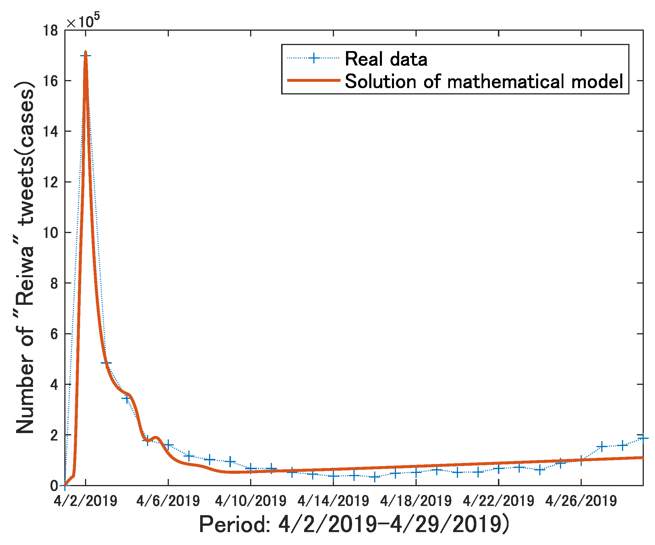
“Reiwa (Beautiful Harmony)”. In Japan, there are both the Christian era and the Japanese imperial era names are used, and when we have new emperor, new era starts. There was a big event in the Japanese royal family this year. Current Emperor Akihito abdicated the throne on 30 April and his son, Crown Prince Naruhito, enthroned the throne on May 1. New Imperial era “Reiwa (Beautiful Harmony)” is taken from a verse in the oldest anthology of poems called Manyo-shu. Here, we used Twitter data after the name of new Imperial era was announced on April 1 to test public interest of new Imperial era “Reiwa” for the fit of the proposed model to actual data.
The actual data in Figure 5 show a rapid, sharp spike followed by an easing, which is a characteristic pattern of transitory booms. The graph from the proposed model fits the actual data with a very high overall accuracy. The high degree of accuracy in the fitness is evident from the value of the coefficient of determination, . In particular, the solution from the proposed model even expresses the small decline that occurs from 4/4/2019 to 4/6/2019. On the other hand, from the graph of the solution to the proposed model, we can see interests of Twitter users of new Imperial era “Reiwa” towards the date when the Era name changes from “Heisei” to “Reiwa”. Thus, we believe that an advantage of the proposed model is its ability to express oscillations by incorporating time delays and “Sakura” data. Moreover, in this example the parameters in Table 5 do not satisfy conditions in Theorem 1, and the numerical solution made from these parameters begins to oscillate halfway and explosively diverges.
6. Conclusions
In this paper, based on our previous study, we examined the mathematical properties, especially the stability of the equilibrium to the reduced model of our proposed model. Moreover, we also used actual data representing transient booms and resurgent booms and conducted parameter estimation for the proposed model using Bayesian inference approach (MCMC-MH methods). In addition, we conducted a model fitting to actual data. By this study, we reconfirmed that we can express the resurgences or slightly oscillations of actual data by means of our proposed model. However, our proposed model was unable to capture secondary peak and detect slight oscillations, as we had expected. The main difficulty is that the mathematical model using the ordinary differential equation will have fewer reproducibility in terms of the actual data involving more peaks or valleys. Although it is difficult to express all peaks or valleys by proposed model, we will be able to reproduce the important peaks or valleys by considering information of the actual data and adjusting , which express time delays, and , which express resurgences. Moreover, it is thought that technique of the sampling using MCMC to evaluate parameters has a difficulty. In our future work, we will try to capture peaks or valleys of the actual data by dividing the timeline into pieces and evaluating the parameter for each piece by Bayesian inference approach.
In addition, there are several potential extensions of the present method. The first one is the validity of the proposed model. This study and our previous study only tested a total of 10 cases. In our future work, it will be necessary to take various examples of boom data, test the validity of our proposed model, and address the relationship between the actual data and parameters. Additionally, we would like to conduct an analysis using data not just for domestic booms but also global booms to test the validity of our proposed model.
The expansion of the model is also an important topic. In particular, a mathematical model should be developed that incorporates probabilistic items to handle unexpected events. The “Sakura” parameter is a unique point of the proposed model, but realistically, a model is needed for scenarios other than that with a constant presence of “Sakura”. We also must consider models with functions that have time-dependent parameters and time-dependent “Sakura”. Moreover, we must also advance mathematical analysis of areas such as the asymptotic behavior of mathematical models and their behavior around the points of equilibrium. In this study, we derived a sufficient condition in regards to the stability of the equilibrium for the reduced model. In the parameter fitting to five actual data for societal booms, “Cup-noodle” and “Reiwa” did not satisfy this sufficient condition. In fact, it was shown that the numerical solution of “Reiwa” begins to oscillate halfway and explosively diverges. However, it is interesting that the numerical solution of “Cup-noodle” converges stably to the equilibrium point. This result implies the improvement of the sufficient condition of the stability in our future challenges.
In recent years, the development of technology has made it relatively easy to obtain large data (both quantitatively and qualitatively), but a significant challenge has been how to use this large amount of data. We would like to continue research efforts in anticipation of the practical contribution of the mathematical model and parameter estimation method using a Bayesian inference approach in this study to corporate marketing strategies.
Author Contributions
Conceptualization, Y.O.; methodology, Y.O. and N.M.; software, Y.O.; validation, Y.O. and N.M.; formal analysis, Y.O.; investigation, Y.O.; resources, Y.O. and N.M.; data curation, Y.O.; writing—original draft preparation, Y.O.; writing—review and editing, Y.O. and N.M.; visualization, Y.O. and N.M. All authors have read and agreed to the published version of the manuscript.
Funding
This work was supported by JSPS KAKENHI Grant Number 18K03439 and 17K04029.
Acknowledgments
The author would like to thank the referees for carefully reading our manuscript and for giving such constructive comments which substantially helped improving the quality of our paper. Moreover, the author wish to thank the Editor for helpful cooperation that have improved the layout of the paper. The first author would like to acknowledge the supports from JSPS Grant-in-Aid for Scientific Research (C) 18K03439 and the second author would like to acknowledge the supports from JSPS Grant-in-Aid for Scientific Research (C) 17K04029.
Conflicts of Interest
The authors declare that they have no conflict of interest regarding the publication of the research article.
References
- Anderson, R.M. Discussion: The Kermack–McKendrick epidemic threshold theorem. Bull. Math. Biol. 1991, 53, 1–32. [Google Scholar] [CrossRef]
- Busenberg, S.; Cooke, K. Vertically Transmitted Diseases Models and Dynamics; Springer: Berlin, Germany, 1993. [Google Scholar]
- Dietz, K. The first epidemic model A historical note on P.D. En’ko. Aust. J. Stat. 1988, 30, 56–65. [Google Scholar] [CrossRef]
- Kermack, W.O.; McKendrick, A.G. Contributions to the mathematical theory of epidemics—I. Proc. R. Soc. 1927, 115, 700–721. [Google Scholar]
- Ishii, A.; Arakaki, H.; Matsuda, N.; Umemura, S.; Urushidani, T.; Yamagata, N.; Yoshida, N. The ’hit’ phenomenon: A mathematical model of human dynamics interactions as a stochastic process. New J. Phys. 2012, 14, 063018. [Google Scholar] [CrossRef]
- Abdullah, S.; Wu, X. An Epidemic Model for News Spreading on Twitter. In Proceedings of the 2011 23rd IEEE International Conference on Tools with Artificial Intelligence, Boca Raton, FL, USA, 7–9 November 2011; Volume 1, pp. 163–169. [Google Scholar]
- Nakagiri, Y.; Kurita, O. On a differential equation model of booms. Trans. Oper. Res. Soc. Jpn. 2004, 47, 83–105. (In Japanese) [Google Scholar] [CrossRef] [Green Version]
- Ueda, Y.; Asahi, Y. Construction and verification for the interest shift model of Twitter users [Twitter-riyousya no kanshin-ikou model no kouchiku to kenshou]. Oper. Res. Manag. Sci. Res. 2014, 59, 219–228. (In Japanese) [Google Scholar]
- Ota, Y.; Mizutani, N. A proposal of mathematical model on booms for human and social life—Using diffusion of innovation theory and delay differential equations. Trans. Oper. Res. Soc. Jpn. 2020. to appear (In Japanese) [Google Scholar]
- Rogers, E.M. The Diffusion of Innovations, 5th ed.; The Free Press: New York, NY, USA, 2003. [Google Scholar]
- Hutchinson, G.E. Circular causal systems in ecology. Ann. N. Y. Acad. Sci. 1948, 50, 221–246. [Google Scholar] [CrossRef]
- May, R.M. Stability and Complexity in Model Ecosystems; Princeton University Press: Princeton, NJ, USA, 1974. [Google Scholar]
- Nicholson, A.J. The Self-Adjustment of Populations to Change. Cold Spring Harb Symp. Quant. Biol. 1957, 22, 153–173. [Google Scholar] [CrossRef]
- Cooke, K.L. Stability analysis for a vector disease model. Rocky Mount. J. Math. 1979, 9, 31–42. [Google Scholar] [CrossRef]
- Mena-Lorcat, J.; Hethcote, H.W. Dynamic models of infectious diseases as regulators of population sizes. J. Math. Biol. 1992, 30, 693–716. [Google Scholar] [CrossRef] [PubMed]
- Pyragas, K. Continuous control of chaos by self-controlling feedback. Phys. Lett. A 1992, 170, 421–428. [Google Scholar] [CrossRef]
- Smith, H.L. Subharmonic bifurcation in an S-I-R epidemic model. J. Math. Biol. 1983, 17, 163–177. [Google Scholar] [CrossRef] [PubMed]
- Kaipio, J.; Somersalo, E. Statistical and Computational Inverse Problems; Springer: New York, NY, USA, 2005. [Google Scholar]
- Robert, C.; Casella, G. Monte Carlo Statistical Methods; Springer: New York, NY, USA, 2004. [Google Scholar]
- Andersson, H.; Britton, T. Stochastic Epidemic Models and their Statistical Analysis; Springer: New York, NY, USA, 2000. [Google Scholar]
- Andrieu, C.; de Freitas, N.; Doucet, A.; Jordan, M.I. An Introduction to MCMC for Machine Learning. Mach. Learn. 2003, 50, 5–43. [Google Scholar] [CrossRef] [Green Version]
- Haario, H.; Laine, M.; Lehtinen, M.; Saksman, E.; Tamminen, J. Markov chain Monte Carlo methods for high dimensional inversion in remote sensing. J. R. Stat. Soc. B Stat. Methodol. 2004, 66, 591–608. [Google Scholar] [CrossRef]
- Jacquier, E.; Jarrow, R. Bayesian analysis of contingent claim model error. J. Econom. 2000, 94, 145–180. [Google Scholar] [CrossRef]
- Jacquier, E.; Polson, N. Bayesian methods in finance. In Oxford Handbook of Bayesian Econometrics; Oxford University Press: Oxford, UK, 2010; pp. 439–512. [Google Scholar]
- Martin, J.C.; Wilcox, L.C.; Burstedde, C.; Ghattas, O. A stochastic Newton MCMC method for large-scale statistical inverse problems with application to seismic inversion. SIAM J. Sci. Comput. 2012, 34, A1460–A1487. [Google Scholar] [CrossRef]
- Michelot, T.; Blackwell, P.G.; Jammes, S.C.; Matthiopoulos, J. Inference in MCMC step selection models. J. Int. Biom. Soc. 2019, 76, 438–447. [Google Scholar] [CrossRef]
- O’Neill, P.D.; Roberts, G.O. Bayesian inference for partially observed stochastic epidemics. J. R. Stat. Soc. A 1999, 162, 121–129. [Google Scholar] [CrossRef]
- Tunaru, R.; Zheng, T. Parameter estimation risk in asset pricing and risk management: A Bayesian approach. Int. Rev. Financ. Anal. 2017, 53, 80–93. [Google Scholar] [CrossRef]
- Wang, J.; Zabaras, N. A Bayesian inference approach to the inverse heat conduction problem. Int. J. Heat Mass Transf. 2004, 47, 3927–3941. [Google Scholar] [CrossRef]
- Levenberg, K. A method for the solution of certain non-linear problems in least squares. Q. Appl. Math. 1944, 2, 164–168. [Google Scholar] [CrossRef] [Green Version]
- Marquardt, D. An algorithm for least-squares estimation of nonlinear parameters. SIAM J. Appl. Math. 1963, 11, 431–441. [Google Scholar] [CrossRef]
- Gelman, A.; Bois, F.; Jiang, J. Physiological pharmacokinetic analysis using population modeling and informative prior distributions. J. Am. Stat. Assoc. 1996, 91, 1400–1412. [Google Scholar] [CrossRef]
- Girolami, M. Bayesian inference for differential equations. Theor. Comput. Sci. 2008, 408, 4–16. [Google Scholar] [CrossRef] [Green Version]
- Hastings, W.K. Monte Carlo sampling methods using Markov chains and their application. Biometrika 1970, 57, 97–109. [Google Scholar] [CrossRef]
- Metropolis, N.; Rosenbluth, A.W.; Rosenbluth, M.N.; Teller, A.H.; Teller, E. Equations of state calculations by fast computing machines. J. Chem. Phys. 1953, 21, 1087–1092. [Google Scholar] [CrossRef] [Green Version]
Figure 1.
Fitting to La La Land data.
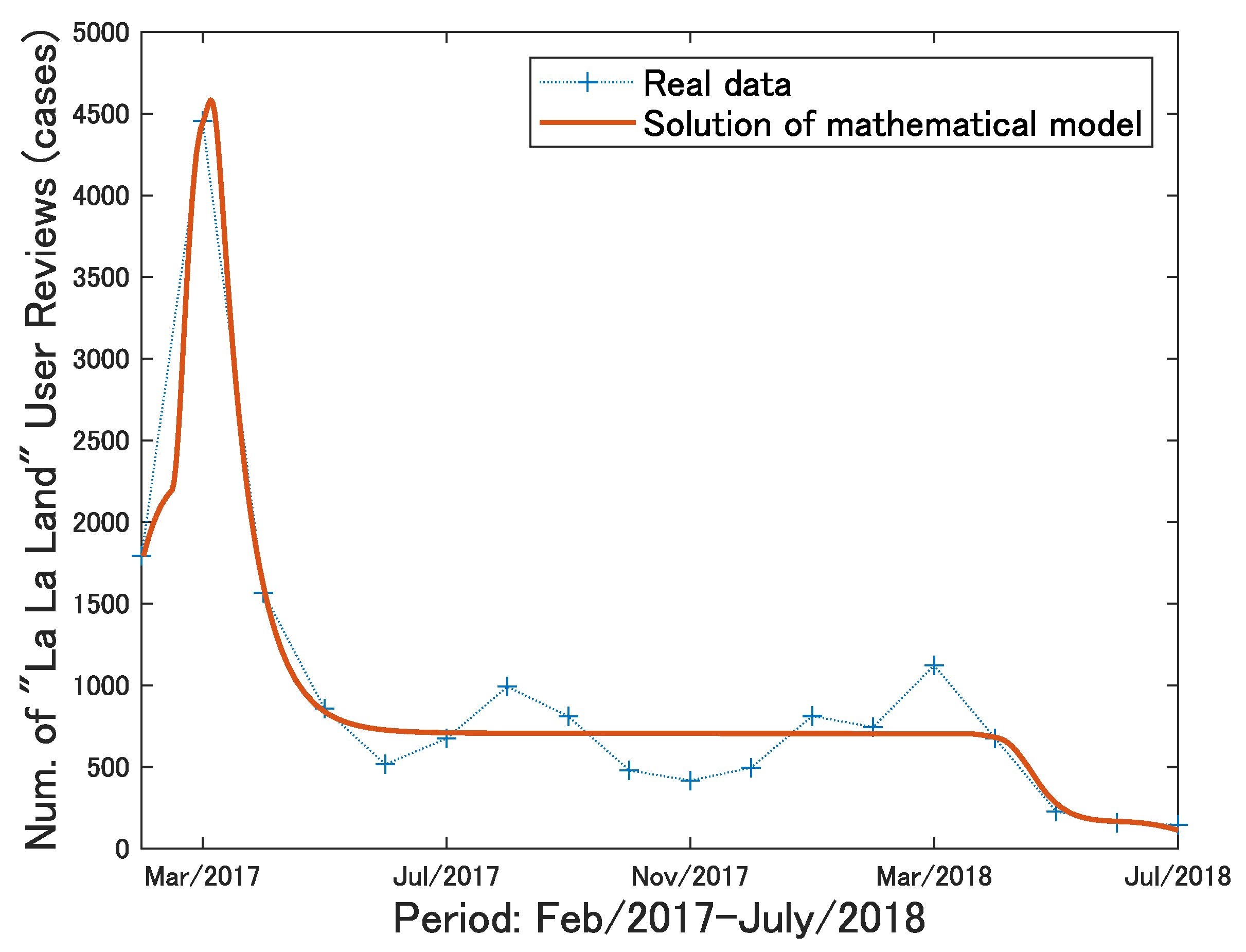
Figure 2.
Fitting to “Ten-nensui” data.
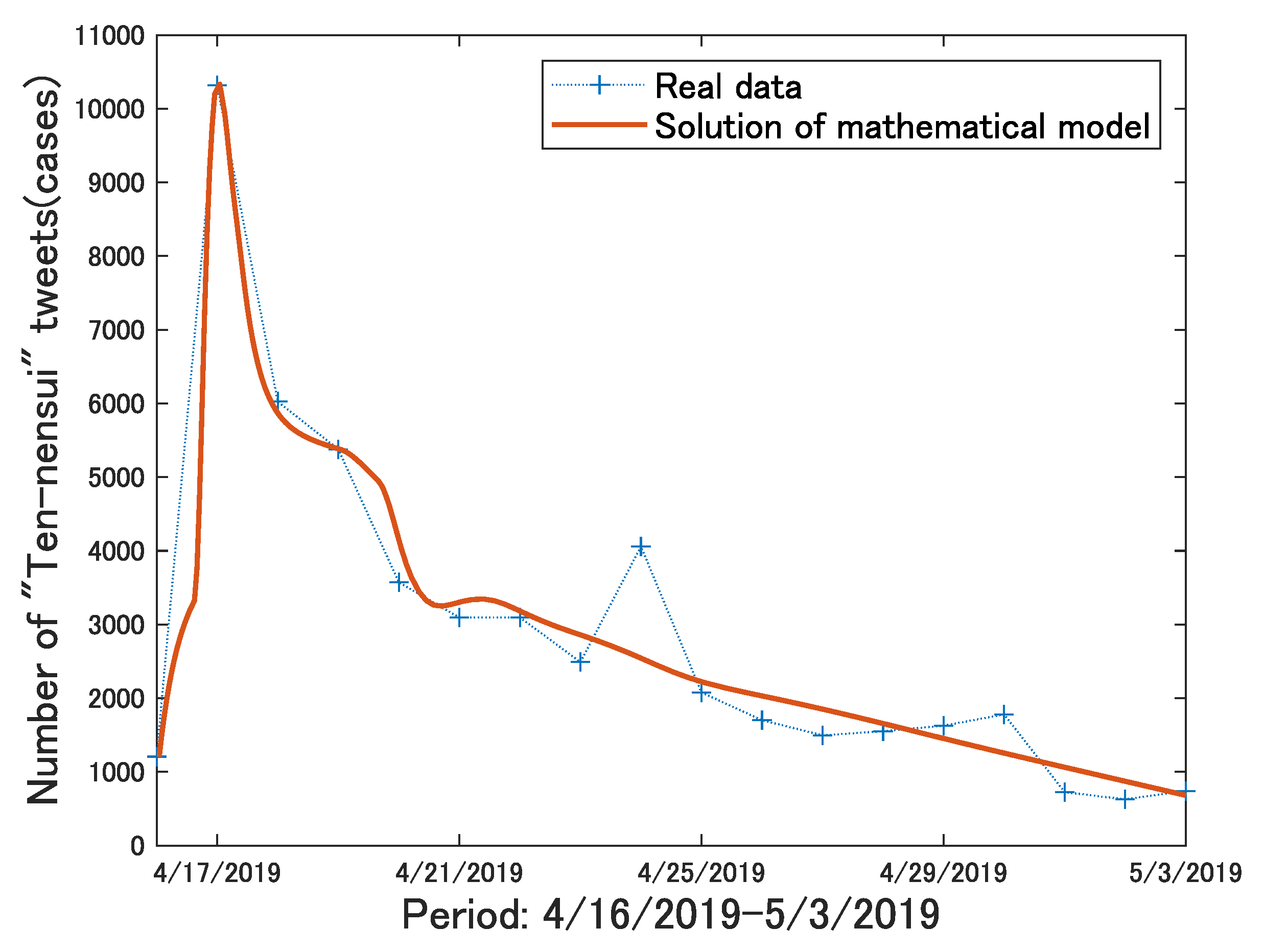
Figure 3.
Fitting to “Honkirin” data.
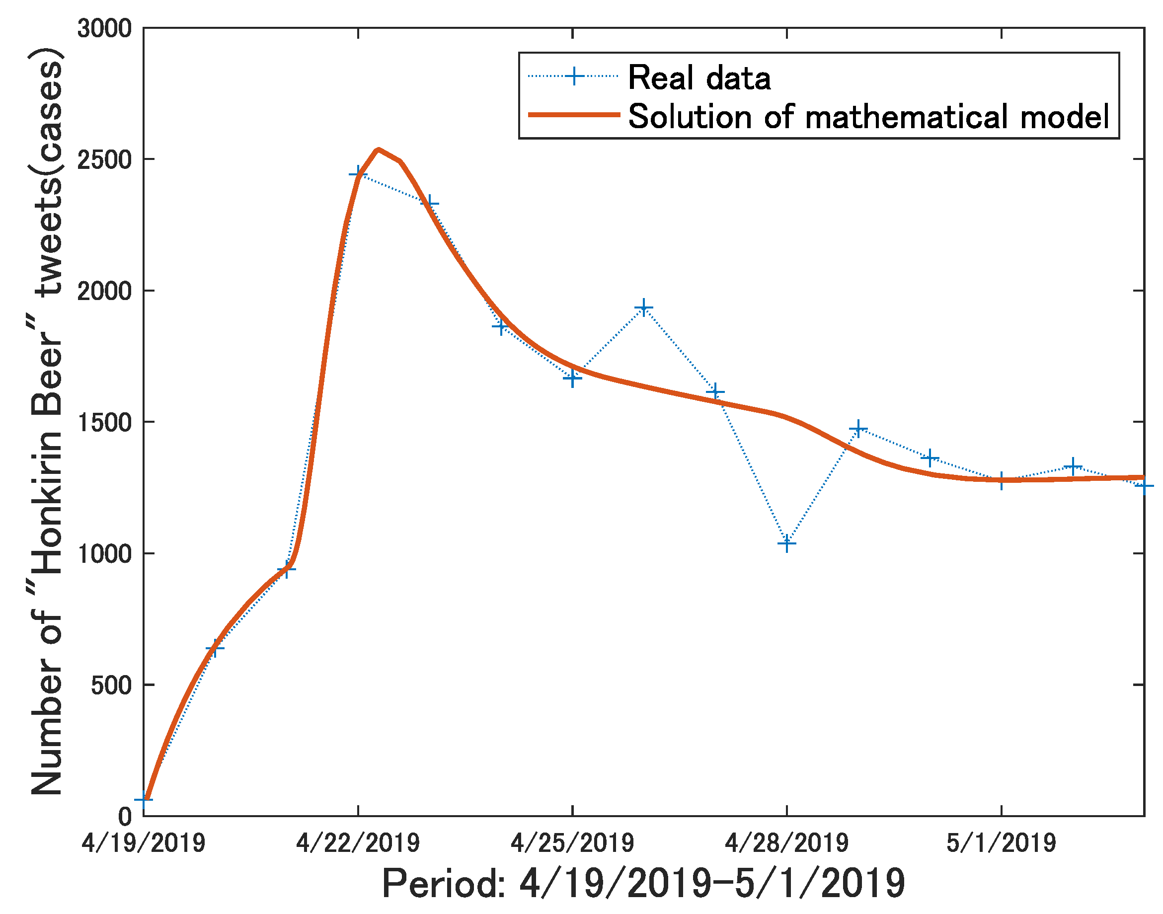
Figure 4.
Fitting to Cup-noodle data.
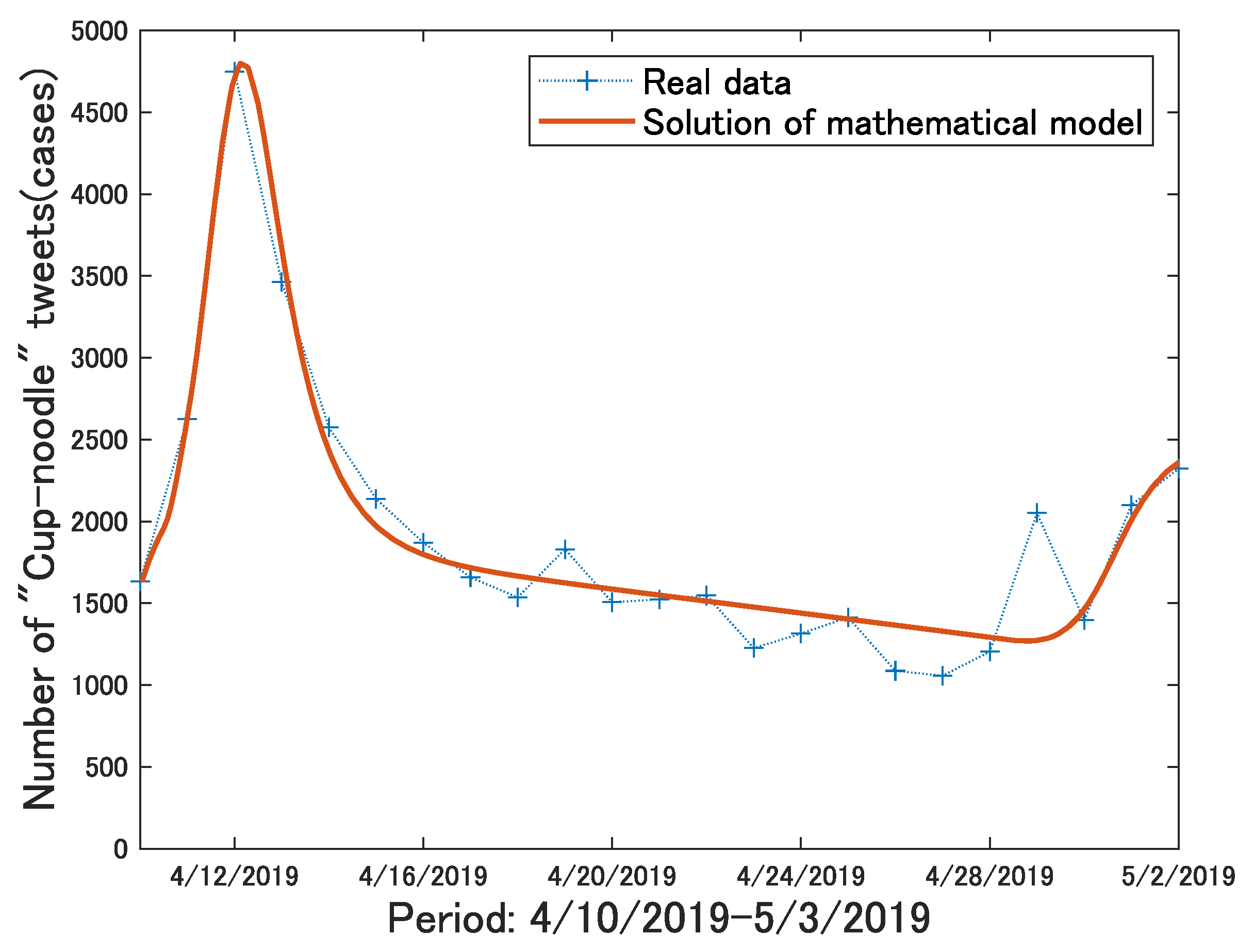
Figure 5.
Fitting to “Reiwa” data.

Table 1.
Various parameter values.
| Lalaland | |||||
|---|---|---|---|---|---|
| 0.0001 | 6700 | ||||
| 0.001 | 0 | ||||
| 0.01 | 1792 | ||||
| 0.001 | 0 | ||||
| 0.001 | 14 | ||||
| 0.001 | 405 | ||||
Table 2.
Various parameter values.
| Pure_Water | |||||
|---|---|---|---|---|---|
| 0.0001 | 19,000 | ||||
| 0.01 | 0 | ||||
| 0.01 | 1207 | ||||
| 0.01 | 0 | ||||
| 0.01 | 14 | ||||
| 0.01 | 72 | ||||
Table 3.
Various parameter values.
| Honkirin Beer | |||||
|---|---|---|---|---|---|
| 0.0001 | 4700 | ||||
| 0.01 | 0 | ||||
| 0.01 | 63 | ||||
| 0.01 | 0 | ||||
| 0.01 | 48 | ||||
| 0.01 | 158 | ||||
Table 4.
Various parameter values.
| Cupnoodle | |||||
|---|---|---|---|---|---|
| 0.0001 | 8200 | ||||
| 0.01 | 0 | ||||
| 0.01 | 1633 | ||||
| 0.01 | 0 | ||||
| 0.01 | 11 | ||||
| 0.01 | 444 | ||||
Table 5.
Various parameter values.
| Beautiful_Harmony | |||||
|---|---|---|---|---|---|
| 0.00001 | 2,700,000 | ||||
| 0.01 | 0 | ||||
| 0.01 | 0 | ||||
| 0.01 | 0 | ||||
| 0.01 | 10 | ||||
| 0.01 | 62 | ||||
© 2020 by the authors. Licensee MDPI, Basel, Switzerland. This article is an open access article distributed under the terms and conditions of the Creative Commons Attribution (CC BY) license (http://creativecommons.org/licenses/by/4.0/).
Share and Cite
MDPI and ACS Style
Ota, Y.; Mizutani, N. Estimating Parameters in Mathematical Model for Societal Booms through Bayesian Inference Approach. Math. Comput. Appl. 2020, 25, 42. https://doi.org/10.3390/mca25030042
AMA Style
Ota Y, Mizutani N. Estimating Parameters in Mathematical Model for Societal Booms through Bayesian Inference Approach. Mathematical and Computational Applications. 2020; 25(3):42. https://doi.org/10.3390/mca25030042
Chicago/Turabian StyleOta, Yasushi, and Naoki Mizutani. 2020. "Estimating Parameters in Mathematical Model for Societal Booms through Bayesian Inference Approach" Mathematical and Computational Applications 25, no. 3: 42. https://doi.org/10.3390/mca25030042