Uniqueness of Closed Equilibrium Hypersurfaces for Anisotropic Surface Energy and Application to a Capillary Problem

Institute of Mathematics for Industry, Kyushu University, Motooka Nishi-ku, Fukuoka 819-0395, Japan
Math. Comput. Appl. 2019, 24(4), 88; https://doi.org/10.3390/mca24040088
Submission received: 22 September 2019
/
Accepted: 6 October 2019
/
Published: 10 October 2019
(This article belongs to the Special Issue Related Problems of Continuum Mechanics)
Abstract
:We study a variational problem for hypersurfaces in the Euclidean space with an anisotropic surface energy. An anisotropic surface energy is the integral of an energy density that depends on the surface normal over the considered hypersurface, which was introduced to model the surface tension of a small crystal. The purpose of this paper is two-fold. First, we give uniqueness and nonuniqueness results for closed equilibria under weaker assumptions on the regularity of both considered hypersurfaces and the anisotropic surface energy density than previous works and apply the results to the anisotropic mean curvature flow. This part is an announcement of two forthcoming papers by the author. Second, we give a new uniqueness result for stable anisotropic capillary surfaces in a wedge in the three-dimensional Euclidean space.
1. Introduction
We study equilibrium hypersurfaces in the -dimensional Euclidean space for anisotropic surface energy, which serve as a mathematical model of small crystals and small liquid crystals with anisotropy. Therefore, the objects of our study should be not only smooth hypersurfaces but also hypersurfaces with singular points like vertices and edges. However, such equilibrium hypersurfaces with both smooth curved parts and singular points have not yet been studied sufficiently well. One of the purposes of this paper is to give a new concept a piecewise- weak immersion and to study variational problems in this class of hypersurfaces. Piecewise- weak immersions are hypersurfaces with the weakest regularity in order to study this type of variational problem by using essentially classical differential geometry. The other purpose of this paper is to give a new uniqueness result for stable anisotropic capillary surfaces in a wedge in , which is proved by using the method developed to pursue the first purpose together with careful treatment of the boundary part by using several new formulas.
Let be a positive continuous function on the unit sphere in . Let X be a closed hypersurface in for which the tangent hyperplane is well defined at almost every point. X will be represented as a mapping from an n-dimensional oriented connected compact manifold M into . Let be the unit normal vector field along , where is the set of singular points of X. The anisotropic energy of X is defined as , where is the n-dimensional volume form of M induced by X. Such an energy was introduced by Gibbs (1839–1903) in order to model the shape of small crystals, and it is used as a mathematical model of anisotropic surface energy [1,2]. It is known that, for any positive number , among all closed hypersurfaces as above enclosing the same -dimensional volume V, there exists a unique (up to translation in ) minimizer of [3]. The minimizer for the specific value is called the Wulff shape for , and we will denote it by . When , is the usual n-dimensional volume of the hypersurface X and is the unit sphere .
In this paper, we study variational problems for the anisotropic energy . In general, the Wulff shape and equilibrium hypersurfaces of such an energy for volume-preserving variations are not smooth. In view of the origin of the energy functional mentioned above, it is natural to try to study the problem under the lowest possible regularities of the considered hypersurfaces and the energy density function. In order to pursue it, we define a new concept “piecewise- weakly immersed hypersurface” and study the variational problem of the energy for functions on . These assumptions on the regularity are weaker than any previous works that studied variational problems of anisotropic surface energies in differential geometry (cf. References [4,5,6,7,8,9]). Under such a weak regularity assumption, we concentrate upon the problem of uniqueness for closed equilibrium hypersurfaces. In order to give precise statements of our results, we prepare a few words.
For any given convex set having the origin of inside, there exists a Lipschitz continuous function such that the boundary of coincides with the Wulff shape for . However, such is not unique. The “smallest” is called the convex integrand for W (or, simply, convex) (for another equivalent definition, see Section 2).
Each equilibrium hypersurface X of for variations that preserve the enclosed -dimensional volume (we will call such a variation a volume-preserving variation) has constant anisotropic mean curvature. Here, the anisotropic mean curvature of a piecewise- hypersurface X is defined at each regular point of X as (cf. Reference [6,10]) , where is the gradient of and H is the mean curvature of X. If , holds.
We call a piecewise- weakly immersed equilibrium hypersurface X a CAMC (constant anisotropic mean curvature) hypersurface (see Definition 3 for details). A CAMC hypersurface is said to be stable if the second variation of the energy for any volume-preserving variation is nonnegative.
One of the most basic questions is as follows:
Question 1.Is any closed CAMC hypersurface the Wulff shape?
The answer to this uniqueness problem is not affirmative in general [11,12,13]. However, it is expected that, if one of the following “good” conditions (I)–(III) is satisfied, the image of any closed CAMC hypersurface X coincides with the Wulff shape (up to translation and homothety).
- (I)
- X is an embedding; that is, X is an injective mapping.
- (II)
- X is stable.
- (III)
- and the genus of M is 0; that is, M is homeomorphic to .
If we assume that is a smooth, strictly convex hypersurface (that is, the support function of is strictly convex. See Definition 1.), any closed CAMC hypersurface X is also smooth and the above expectation was already proved. In fact, if X satisfies one of (I)–(III), it is a homothety of the Wulff shape (which was proved by the following papers: For (I), Reference [14] for and Reference [5] for general ; for (II), Reference [15] for and Reference [8] for general ; and for (III), Reference [16] for and Reference [7] for general ). However, the situation is not the same for more general and/or . Actually, if is not strictly convex, even if it is convex (See Definition 1) and of class , the Wulff shape can have singular points and its principal curvatures can be unbounded (Example 3). Also, we have the following striking nonuniqueness results.
Theorem 1
([17]). There exists a function such that there exist closed embedded CAMC hypersurfaces in for γ, each of which is not (any homothety or translation of) the Wulff shape .
Theorem 2
([17]). There exists a function such that there exist closed embedded CAMC surfaces in with genus zero for γ, each of which is not (any homothety or translation of) the Wulff shape .
Theorems 1 and 2 are proved by giving suitable examples (Section 4). The same examples give self-similar shrinking solutions with genus 0 for anisotropic mean curvature flow, which are not (any homotheties or translations of) the Wulff shape (Section 6). In contrast with this, the round sphere is the only closed embedded self-similar shrinking solution of the mean curvature flow in with genus zero [18].
As for the uniqueness of stable closed CAMC hypersurfaces, we obtain the following result.
Theorem 3
Let us mention the preceding works relating to Theorem 3. As for planer curves, Morgan [20] proved that, if is continuous and convex, then any closed equilibrium rectifiable curve for in is (up to translation and homothety) a covering of the Wulff shape. About uniqueness of closed stable equilibria in , Palmer [9] proved the same result as Theorem 3 but under the assumptions that is of and that considered surfaces and the Wulff shape satisfy some extra assumptions.
A similar method to prove Theorem 3 together with careful treatment on the free boundary gives a uniqueness result for a capillary problem. For simplicity, we assume that is a strictly convex function of class . Let be a wedge-shaped domain bounded by two planes , in , and let be a positive constant. Let M be a two-dimensional oriented connected compact manifold with boundary , where each is a topological circle. Consider any -immersion of which the restriction to is an embedding. Set , and let be the domain bounded by (). We define the wetting energy of X as follows:
where is the area of . Then, we define the total energy of X by
Note that is a piecewise smooth surface without boundary. We denote by the oriented volume enclosed by . We call a critical point of E for volume-preserving variations an anisotropic capillary surface (or, simply, a capillary surface). A capillary surface is said to be stable if the second variation of E is nonnegative for all volume-preserving variations of X. In the following uniqueness theorem, we identify M with .
Theorem 4.
Let Ω be a wedge in bounded by two planes and , and let be a compact oriented immersed surface that is disjoint from the edge of Ω, having embedded boundary and satisfying for a nonempty bounded domain in . If M is a stable anisotropic capillary surface in and both and are convex, then M is (up to translation and homothety) part of the Wulff shape . Conversely, if M is part of (up to translation and homothety), then it is stable.
As for previous works which are closely related to Theorem 4, we have the following. We studied the existence and uniqueness of stable anisotropic capillary surfaces between two parallel planes and in [21,22,23]. Moreover, in Reference [24], we proved the uniqueness result similar to Theorem 4 for isotropic capillary hypersurfaces in a wedge in ; here, isotropic means that .
This article is organized as follows. In Section 2, we give the definition and a representation of the Wulff shape and some fundamental concepts relating to the Wulff shape. Also some typical examples are given. In Section 3, we give the Euler–Lagrange equations for our variational problem and the definitions of anisotropic curvatures. In Section 4, we give outlines of the proofs of Theorems 1 and 2. In Section 5, an outline of the proof of Theorem 3 is given. In Section 6, we mention an application to anisotropic mean curvature flow. In Section 7, we give the proof of Theorem 4.
2. Preliminaries
Let be a positive continuous function. In this paper, we call the boundary of the convex set the Wulff shape for , where means the standard inner product in . In other literatures, is often called the Wulff shape.
From now on, any parallel translation of the Wulff shape will be also called the Wulff shape, and it will be denoted also by , if it does not cause any confusion.
Let us define two terminologies which represent the convexity of the energy density function .
Definition 1.
(i) (cf. References [3,25]) A continuous map is called a convex integrand (or, simply, convex) if its homogeneous extension defined by
is a convex function.
(ii) If is of class , we say that γ is strictly convex if the matrix is positive definite at any point in ; here, is the Hessian of γ on and is the identity matrix of size n.
The Wulff shape is not smooth, in general. It is smooth and strictly convex (that is, each principal curvature of with respect to the inward-pointing normal is positive at each point of ) if and only if is of class and strictly convex. On the other hand, if is of class , is convex if and only if is positive semi-definite. For such , the Wuff shape can have singular points as Example 3 shows.
Assume that is of class . The Cahn–Hoffman map for is defined as , (). Here, the tangent space of at is naturally identified with a hyperplane in . If is convex, the image coincides with ; that is, gives a representation of .
Here, we give four typical examples. We denote a point in by .
Example 1.
Define a function as . Then, γ is convex and (). Hence, .
Example 2.
Define a function as . Then, and convex and the Wulff shape is the cube
Since γ is differentiable only at points except points in , the Cahn–Hoffman map is defined on and the image of is the set of all vertices of the cube .
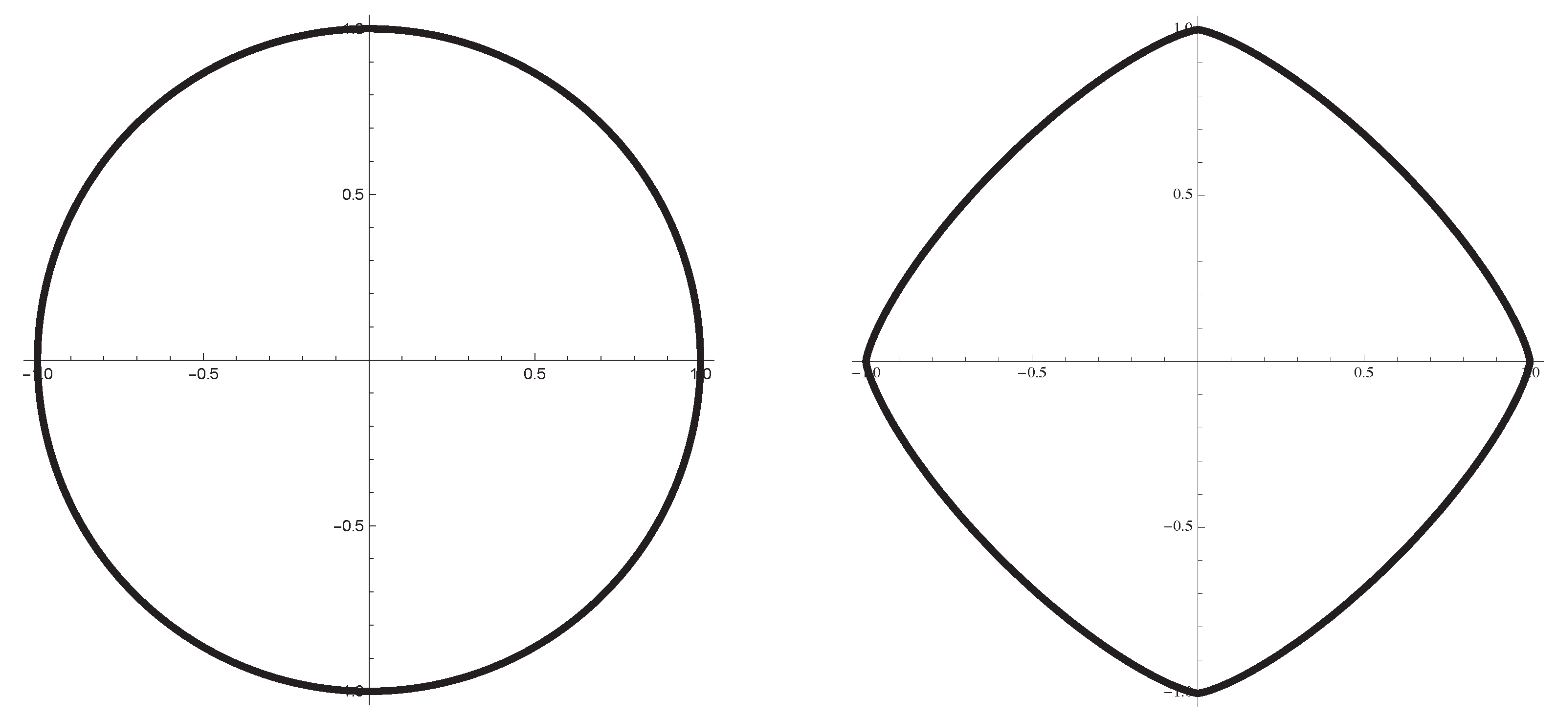
Example 3
([19]). We give a simple example, which shows that, if the energy density function γ is not strictly convex, even if it is convex, the Wulff shape can have singular points and its principal curvatures can be unbounded. Set . For , define
Then, is of class and convex. Hence, the Wulff shape and the image of the Cahn–Hoffman map for coincide, and they are shown in Figure 1. is represented as
Moreover, we have
Hence, the following can be stated.
- (i)
- If , on .
- (ii)
- is positive definite on and positive semi-definite on .
The curvature of with respect to the outward-pointing normal ν is represented as
Hence, near each point in , is unbounded and the following holds.
Example 4.
We give a nonconvex example of γ. Set . Define γ as . Then, γ is of class and it is not convex. The whole of the closed curve with self-intersection in Figure 2 is the image of the Cahn–Hoffman map , while the closed convex solid curve that is a proper subset of is the Wulff shape . Denote by the curvature of at its regular points with respect to the normal ν. By computation, we obtain
Hence, for any ,
is the set of exactly six points, and it is the set of the singular points of (Figure 2).
3. Euler–Lagrange Equations and Anisotropic Curvatures
From now on, we assume that is of class . Let be an n-dimensional oriented compact connected manifold, where each is an n-dimensional connected compact submanifold of M with piecewise- boundary and (, ). We call a map a piecewise- weak immersion (or a piecewise- weakly immersed hypersurface) if X satisfies the following conditions (A1), (A2), and (A3) for [19].
- (A1)
- X is continuous, and each is of class .
- (A2)
- The restriction of X to the interior of is a -immersion.
- (A3)
- The unit normal vector field along can be extended to a -mapping . Here, the orientation of is determined so that, if is a local coordinate system in , then gives the canonical orientation in .
The Cahn–Hoffman field along for is defined as . Note that the Cahn–Hoffman map is a front ([19]). Hence the “tangent space” of the image at each point can be defined. Since the unit normal of at coincides with the unit normal of at the point , we can identify with .
The linear map given by the matrix is called the anisotropic shape operatior of . Various anisotropic curvatures of X are defined as follows.
Definition 2
(anisotropic curvatures; cf. References [5,10]). (i) The eigenvalues of are called the anisotropic principal curvatures of X. We denote them by .
(ii) Let be the elementary symmetric functions of :
Set . is called the rth anisotropic mean curvature of X, where .
(iii) is called the anisotropic mean curvature of X, and we often denote it by Λ; that is, .
The anisotropic curvatures of the most fundamental hypersurfaces and are simply stated as follows.
Remark 1
([6,19]). For the Cahn–Hoffman map , , (), it is shown that the unit normal vector field is given by . Hence, the anisotropic shape operator of is . Therefore, the anisotropic principal curvatures of are , and hence, each rth anisotropic mean curvature of is . Particularly, the anisotropic mean curvature of for the normal ν and that of for the outward-pointing unit normal is at any regular point.
is not symmetric in general. However, we have the following good properties of the anisotropic curvatures.
Remark 2
(i) If is positive definite at a point (), then all of the anisotropic principal curvatures of X at p are real [26].
(ii) is not a real value in general. However, each is always a real valued function on [19].
We have the following first variation formula for the anisotropic surface energy .
Proposition 1
([19]). Assume that the map satisfies (A1), (A2), and (A3) above with , , and . Let (), be a variation of X; that is, and . Assume for simplicity that is of class in ϵ. We also assume that, for each , the anisotropic mean curvature of () is bounded on . Set
Then, the first variation of the anisotropic energy is given as follows.
where is the -dimensional volume form of induced by X, N is the outward-pointing unit conormal along , R is the -rotation on the -plane, p is the projection from to the -plane, and the first integral in the right hand side of Equation (4) which is an improper integral converges.
On the other hand, the first variation of the -dimensional volume enclosed by is
(cf. Reference [27]). This with Equation (4) gives the following Euler–Lagrange equations.
Proposition 2
(Euler–Lagrange equations, Koiso [19]. For , see Palmer [9]). A piecewise- weak immersion is a critical point of the anisotropic energy for volume-preserving variations if and only if the following conditions (i) and (ii) hold.
(i) The anisotropic mean curvature of X is constant on .
(ii) holds at any , where a tangent space of a submanifold of is naturally identified with a linear subspace of .
In view of Proposition 2, we will use the following terminology.
Definition 3
([19]). A piecewise- weak immersion is called a hypersurface with constant anisotropic mean curvature (CAMC) if both conditions (i) and (ii) in Proposition 2 hold.
4. Outline of the Proofs of Theorems 1 and 2
Theorems 1 and 2 are proven by giving explicit examples [17]. Here, we give an example for . Consider the function defined by
By computation, the corresponding Cahn–Hoffman map is given as follows.
where . The image of is shown in Figure 3, left. It is a surface of revolution, and we show by the right figure in Figure 3 its section in the -plane. In Figure 4, we show three closed embedded surfaces of revolution with genus 0, each of which is a subset of . Since the anisotropic mean curvature of is for the unit normal (Remark 1), all of these three surfaces have constant anisotropic mean curvature . The surface in Figure 3a is the Wulff shape , and the surfaces in Figure 3b,c are closed piecewise- CAMC surfaces for , which are not the Wulff shape (up to homothety and translation). These two surfaces give the proof of Theorems 1 and 2 for .
The section of and that of in the -plane (Figure 3, right) give an example to prove Theorem 1 for . Suitable rotations of give a proof of Theorem 1 for similar to the above discussion for .
5. Outline of the Proof of Theorem 3
In this section, first, we give two useful integral formulas that are generalizations of the Steiner formula and the Minkowski formula (see Reference [26] for smooth case). They are proven in Reference [19] and are used to prove Theorem 3.
“Anisotropic parallel hypersurface” is a generalization of parallel hypersurface and is defined as follows.
Definition 4
(Anisotropic parallel hypersurface, cf. Reference [10]). Let X be a piecewise- weak immersion. For any real number t, we call the map the anisotropic parallel deformation of X of height t. If is a piecewise- weak immersion, then we call it the anisotropic parallel hypersurface of X of height t.
The anisotropic energy of the anisotropic parallel hypersurface is a polynomial of t with degree at the most n as follows.
Theorem 5
(Steiner-type formula [19]). Assume that is of class . Let be a piecewise- weak immersion. Consider anisotropic parallel hypersurfaces , where is the set of singular points of X. Then, the following integral formula holds.
where means .
The isotropic version of Theorem 5 is known as the Weyl’s tube formula [28]. The isotropic 2-dimensional version is the well-known Steiner’s formula.
Next, we give a generalization of the Minkowski formula.
Theorem 6
(Minkowski-type formula [19]). Assume that is of class . Assume also that is a closed piecewise- weak immersion and that X satisfies the following condition.
where is the Cahn–Hoffman field along and the tangent space of a submanifold of is naturally identified with a linear subspace of . Then, we have the following integral formulas.
(i)
(ii) Assume that the rth anisotropic mean curvature of X for γ is integrable on M for . Then,
holds, where is the rth anisotropic mean curvature of X.
Now, let us give an outline of the proof of Theorem 3. We first prove that the Cahn–Hoffman field along a closed CAMC hypersurface can be defined as a continuous map on the whole of M. Then, we consider the anisotropic parallel hypersurfaces (, ) of X. By taking homotheties of if necessary, we have a volume-preserving variation (, ) of X. Using Theorems 5 and 6, by long computation, we prove that the following holds: . Since is convex, all are real values on (Remark 2). Hence, if X has constant anisotropic mean curvature and is stable, then must hold on . Therefore, from Corollary 1 in Reference [10], holds for some . Because M is closed and has anisotropic mean curvature , this inclusion implies that the following holds: .
6. Application to Anisotropic Mean Curvature Flow
Let be of class with Cahn–Hoffman map . Let be a one-parameter family of embedded piecewise- hypersurfaces with anisotropic mean curvature . Assume that the Cahn–Hoffman field along is defined as a continuous map on M. If satisfies , it is called an anisotropic mean curvature flow, which diminishes the anisotropic energy if [17]. The example given in Section 4 (see Figure 4b,c) gives self-similar shrinking solutions with genus 0, which are not (any homotheties or translations of) the Wulff shape.
7. Proof of Theorem 4
Most of the work in this section can be generalized to hypersurfaces in . We will discuss it in another paper [29].
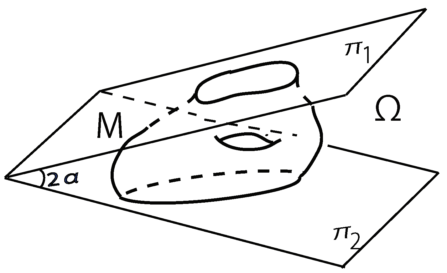
Let and be two planes in containing the -axis and making angles and () with the horizontal plane , respectively. Let be the wedge-shaped domain bounded by and (Figure 5). We denote by the closure of . The -axis is called the edge of the wedge . Denote by the unit normal to which points outward from .
Let be a strictly convex function of class . As in Section 1, let be a -immersion of which the restriction is an embedding onto two simple closed curves and . Denote by the (nonempty) domain bounded by . Then, by a similar way to the way to derive the Euler–Lagrange equations in Reference [22], we can prove the following Euler–Lagrange equations for our capillary problem.
Lemma 1.
X is a capillary surface if and only if both of the following conditions (i) and (ii) hold.
(i) The anisotropic mean curvature Λ of X is constant on M.
(ii) on (), where is the Cahn–Hoffman field along X.
In view of the property of condition (ii) in Lemma 1, it is useful to consider the anisotropic energy for curves in . First, define planes () by
Then, set the following:
Assume that is sufficiently small so that includes at least two distinct points. Then, is a strictly convex closed curve in the plane . We regard the point as the origin of . Denote by the support function of . Then, is the Wulff shape for . For later use, we denote by the Cahn–Hoffman map for .
Now, let be a regular embedded curve with outward unit normal . Define the anisotropic energy of by
where is the line element of .
From now on, we assume that X is a capillary surface. Set the following:
Denote by the outward-pointing unit normal to in the plane . X has the following property, which we call the balancing formula that is a generalization of the balancing formula for the isotropic case [24].
Lemma 2.
Proof.
Let u be a constant vector in . Consider the parallel translations:
Then, by the first variation formulas in Equations (4) and (5), we have
Hence, by setting , , , we have
On , since and hold, we can write
where is tangent to . Then, we have
Note that, by the divergence theorem, the following holds:
Hence, substituting Equation (11) into Equation (10), we obtain
Because , are linearly independent, Equation (12) implies Equation (9). □
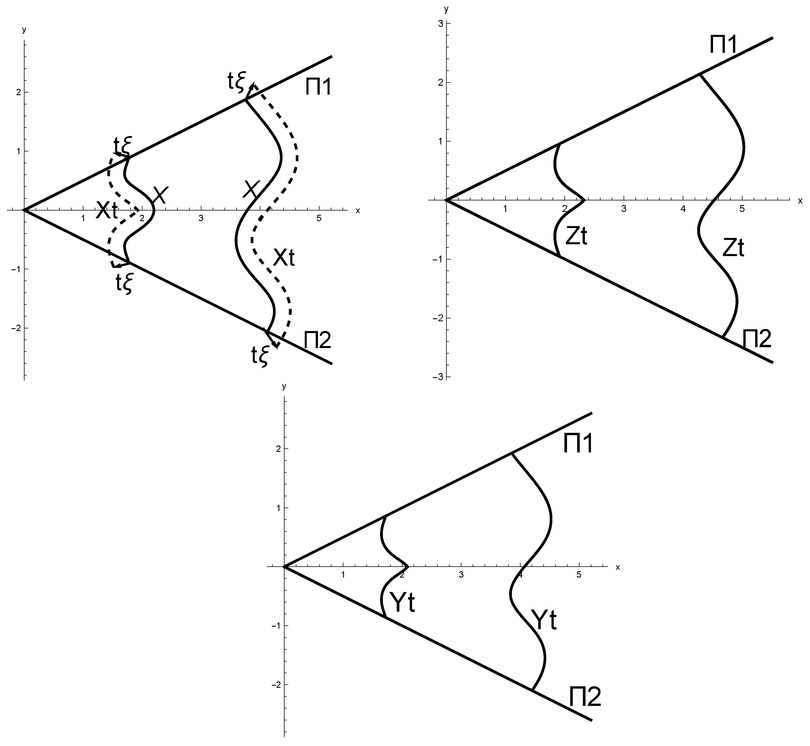
Now, consider the anisotropic parallel surfaces (, ) of X. Set . Then, the variation of X satisfies the boundary condition. Take homotheties
of if necessary so that is a volume-preserving variation of X (Figure 6).
Denote by the total energy of . Then, by a similar way to the proof of Theorem 3, we obtain
where is the anisotropic (mean) curvature of for .
Note that, from Remark 2(i), is real. Since X has constant anisotropic mean curvature , the first term of the right hand side of Equation (13) is nonnegative if and only if . Hence, again by Corollary 1 in Reference [10], holds.
Let us study the second term of the right hand side of Equation (13). Set the following:
We will prove that holds and that the equality holds if and only if for some . Using Equation (9), we obtain
Below, for simplicity, we identify an embedded closed curve in a plane with the domain bounded by this curve.
Since the Wulff shape is the minimizer of among closed curves enclosing the same area, it holds that
where the equality holds if and only if for some . Denote by the Cahn–Hoffman map for and by the line element of . Then, by the definition of and since is the support function of , we have
Let us compute the second term of . For simplicity, we denote by also the Cahn–Hoffman field of . Then, by Equations (4) and (5), we have
Assume now that is convex. Then, for , it holds that
where is a real number depending on and ([30], Theorem 5.1.7). Equation (17) with Equation (18) gives
From Equations (14)–(16) and (19), we obtain
where the equality holds if and only if for some .
If the capillary surface X is stable, then . Hence, by the above observations, holds. Conversely, if is part of a homothety of the Wulff shape , by a similar way to the proof of Theorem 4.1 in Reference [22], it is shown that X is stable, which proves Theorem 4.
Funding
This work was partially supported by JSPS KAKENHI grant number JP18H04487.
Acknowledgments
The author would like to thank the referees for the valuable comments, which helped to improve the manuscript.
Conflicts of Interest
The authors declare no conflict of interest.
References
- Winterbottom, W.L. Equilibrium shape of a small particle in contact with a foreign substrate. Acta Metall. 1967, 15, 303–310. [Google Scholar] [CrossRef]
- Wulff, G. Zur Frage der Geschwindigkeit des Wachsthums und der Auflösung der Krystallflächen. Zeitschrift für Krystallographie und Mineralogie 1901, 34, 449–530. [Google Scholar]
- Taylor, J.E. Crystalline variational problems. Bull. Am. Math. Soc. 1978, 84, 568–588. [Google Scholar] [CrossRef] [Green Version]
- Ando, N. Hartman-Wintner’s theorem and its applications. Calc. Var. Partial Differ. Equ. 2012, 43, 389–402. [Google Scholar] [CrossRef]
- He, Y.; Li, H.; Ma, H.; Ge, J. Compact embedded hypersurfaces with constant higher order anisotropic mean curvatures. Indiana Univ. Math. J. 2009, 58, 853–868. [Google Scholar] [CrossRef] [Green Version]
- Koiso, M.; Palmer, B. Geometry and stability of surfaces with constant anisotropic mean curvature. Indiana Univ. Math. J. 2005, 54, 1817–1852. [Google Scholar] [CrossRef]
- Koiso, M.; Palmer, B. Anisotropic umbilic points and Hopf’s theorem for surfaces with constant anisotropic mean curvature. Indiana Univ. Math. J. 2010, 59, 79–90. [Google Scholar] [CrossRef]
- Palmer, B. Stability of the Wulff shape. Proc. Am. Math. Soc. 1998, 126, 3661–3667. [Google Scholar] [CrossRef]
- Palmer, B. Stable closed equilibria for anisotropic surface energies: Surfaces with edges. J. Geom. Mech. 2012, 4, 89–97. [Google Scholar] [CrossRef]
- Reilly, R.C. The relative differential geometry of nonparametric hypersurfaces. Duke Math. J. 1976, 43, 705–721. [Google Scholar] [CrossRef]
- Kapouleas, N. Complete constant mean curvature surfaces in euclidean three-space. Ann. Math. 1990, 131, 239–330. [Google Scholar] [CrossRef]
- Kapouleas, N. Constant mean curvature surfaces constructed by fusing Wente tori. Invent. Math. 1995, 119, 443–518. [Google Scholar] [CrossRef] [Green Version]
- Wente, H.C. Counterexample to a conjecture of H. Hopf. Pac. J. Math. 1986, 121, 193–243. [Google Scholar] [CrossRef]
- Alexandrov, A.D. A characteristic property of spheres. Annali di Matematica Pura ed Applicata 1962, 58, 303–315. [Google Scholar] [CrossRef]
- Barbosa, J.L.; do Carmo, M. Stability of hypersurfaces with constant mean curvature. Math. Z. 1984, 185, 339–353. [Google Scholar] [CrossRef]
- Hopf, H. Differential Geometry in the Large; Springer: Berlin, Germany, 1989. [Google Scholar]
- Jikumaru, Y.; Koiso, M. Non-uniqueness of closed embedded non-smooth hypersurfaces with constant anisotropic mean curvature. arXiv 2019, arXiv:1903.03958. [Google Scholar]
- Brendle, S. Embedded self-similar shrinkers of genus 0. Ann. Math. 2016, 183, 715–728. [Google Scholar] [CrossRef]
- Koiso, M. Uniqueness of stable closed non-smooth hypersurfaces with constant anisotropic mean curvature. arXiv 2019, arXiv:1903.03951. [Google Scholar]
- Morgan, F. Planar Wulff shape is unique equilibrium. Proc. Am. Math. Soc. 2005, 133, 809–813. [Google Scholar] [CrossRef]
- Koiso, M.; Palmer, B. Stability of anisotropic capillary surfaces between two parallel planes. Calc. Var. Partial Differ. Equ. 2006, 25, 275–298. [Google Scholar] [CrossRef]
- Koiso, M.; Palmer, B. Anisotropic capillary surfaces with wetting energy. Calc. Var. Partial Differ. Equ. 2007, 29, 295–345. [Google Scholar] [CrossRef]
- Koiso, M.; Palmer, B. Uniqueness theorems for stable anisotropic capillary surfaces. SIAM J. Math. Anal. 2007, 39, 721–741. [Google Scholar] [CrossRef]
- Choe, J.; Koiso, M. Stable capillary hypersurfaces in a wedge. Pac. J. Math. 2016, 280, 1–15. [Google Scholar] [CrossRef] [Green Version]
- Morgan, F. The cone over the Clifford torus in R4 is Φ-minimizing. Math. Ann. 1991, 289, 341–354. [Google Scholar] [CrossRef]
- He, Y.; Li, H. Integral formula of Minkowski type and new characterization of the Wulff shape. Acta Math. Sin. 2008, 24, 697–704. [Google Scholar] [CrossRef] [Green Version]
- Barbosa, J.L.; do Carmo, M.; Eschenburg, J. Stability of hypersurfaces of constant mean curvature in Riemannian manifolds. Math. Z. 1988, 197, 123–138. [Google Scholar] [CrossRef]
- Weyl, H. On the volume of tubes. Am. J. Math. 1939, 61, 461–472. [Google Scholar] [CrossRef]
- Koiso, M. Stable anisotropic capillary hypersurfaces in a wedge. In preparation.
- Schneider, R. Convex Bodies: The Brunn–Minkowski Theory; Cambridge University Press: Cambridge, UK, 1993. [Google Scholar]
Figure 1.
On the left, for and, on the right, for for defined by Equation (2).
Figure 1.
On the left, for and, on the right, for for defined by Equation (2).

Figure 2.
The image of the Cahn–Hoffman map for γ in Example 4: The six vertices are the image of the singular points of , and the closed convex solid curve is the Wulff shape .
Figure 2.
The image of the Cahn–Hoffman map for γ in Example 4: The six vertices are the image of the singular points of , and the closed convex solid curve is the Wulff shape .

Figure 3.
Left: The image of the Cahn–Hoffman map for defined by Equation (6). Right: The section of in the -plane.
Figure 3.
Left: The image of the Cahn–Hoffman map for defined by Equation (6). Right: The section of in the -plane.

Figure 4.
Some of the closed surfaces which are subsets of for defined by Equation (6) (Figure 3). The anisotropic mean curvature for the outward-pointing normal is : (a) Wulff shape ; (b) a constant anisotropic mean curvature (CAMC) surface for ; and (c) a CAMC surface for .

Figure 5.
The wedge and an admissible surface M.

Figure 6.
Construction of volume-preserving variation using anisotropic parallel surfaces of X. Upper left: A capillary surface X and its anisotropic parallel surface . Upper right: A parallel translation of that satisfies the boundary condition. Bottom: A homothety of that satisfies the volume condition.

© 2019 by the author. Licensee MDPI, Basel, Switzerland. This article is an open access article distributed under the terms and conditions of the Creative Commons Attribution (CC BY) license (http://creativecommons.org/licenses/by/4.0/).
Share and Cite
MDPI and ACS Style
Koiso, M. Uniqueness of Closed Equilibrium Hypersurfaces for Anisotropic Surface Energy and Application to a Capillary Problem. Math. Comput. Appl. 2019, 24, 88. https://doi.org/10.3390/mca24040088
AMA Style
Koiso M. Uniqueness of Closed Equilibrium Hypersurfaces for Anisotropic Surface Energy and Application to a Capillary Problem. Mathematical and Computational Applications. 2019; 24(4):88. https://doi.org/10.3390/mca24040088
Chicago/Turabian StyleKoiso, Miyuki. 2019. "Uniqueness of Closed Equilibrium Hypersurfaces for Anisotropic Surface Energy and Application to a Capillary Problem" Mathematical and Computational Applications 24, no. 4: 88. https://doi.org/10.3390/mca24040088