Direct Power Control Optimization for Doubly Fed Induction Generator Based Wind Turbine Systems

Abstract

This study presents an intelligent metaheuristics-based design procedure for the Proportional-Integral (PI) controllers tuning in the direct power control scheme for 1.5 MW Doubly Fed Induction Generator (DFIG) based Wind Turbine (WT) systems. The PI controllers’ gains tuning is formulated as a constrained optimization problem under nonlinear and non-smooth operational constraints. Such a formulated tuning problem is efficiently solved by means of the proposed Thermal Exchange Optimization (TEO) algorithm. To evaluate the effectiveness of the introduced TEO metaheuristic, an empirical comparison study with the homologous particle swarm optimization, genetic algorithm, harmony search algorithm, water cycle algorithm, and grasshopper optimization algorithm is achieved. The proposed TEO algorithm is ensured to perform several desired operational characteristics of DFIG for the active/reactive power and DC-link voltage simultaneously. This is performed by solving a multi-objective function optimization problem through a weighted-sum approach. The proposed control strategy is investigated in MATLAB/environment and the results proved the capabilities of the proposed control system in tracking and control under different scenarios. Moreover, a statistical analysis using non-parametric Friedman and Bonferroni–Dunn’s tests demonstrates that the TEO algorithm gives very competitive results in solving global optimization problems in comparison to the other reported metaheuristic algorithms.

1. Introduction

Recently, the increasing consumption of electrical energy, depletion of fossil fuels and the environmental problems related to using the non-renewable sources have promoted a growing interest in renewable energies [1,2]. Wind power as a renewable source represents an important and a promising solution for electrical demand and has recently gained more attention for its significant merits of cleanness and resource abundances. Various wind energy configurations are produced from the intensive studies and researches that are carried out in wind systems. One of the most common configurations is the grid-connected Doubly Fed Induction Generators (DFIGs) equipped with variable speed Wind Turbines (WTs). This configuration was widely installed in wind industry due to its significant merits such as independent control of active and reactive powers, low converters’ costs and mechanical stress reduction [2].

A DFIG is a wound rotor generator in which the stator windings are directly connected to the grid. The rotor windings are connected to the grid through a back-to-back power converter that is composed from the Rotor Side Converter (RSC) and Grid Side Converter (GSC) components. This configuration allows the converter to handle the fraction of 20% to 30% of the total power. Therefore, the losses in the converter are lower compared to a system where the converter has to handle the full power leading to an improvement in the total efficiency [2,3].

However, the switching of Insulated-Gate Bipolar Transistors (IGBTs) at both the RSC and GSC components is usually performed by Sinusoidal Pulse Width Modulation (SPWM) strategy, which generates the high frequency content in the utility current. A simple L-filter or an LCL-filter is adopted to reduce the Total Harmonic Distortion (THD) of the utility current [4]. To meet the grid code requirements, the LCL-filter is predominant in reducing the utility current harmonics. Indeed, it can lead to a better attenuation of harmonics using small values of inductances. However, the resonance phenomena of the LCL-filter must be damped properly in order to prevent the possible instability of these systems [4]. One way for solving this problem is employing a passive damping circuit. The passive damping is built by inserting a resistor branch in series or in parallel with the inductors or capacitors of the LCL-filter [4].

The conventional control scheme of the grid connected DFIG wind turbine system is built based on a vector control method [5,6,7,8]. Here, the Stator Flux Orientation (SFO) scheme is selected for DFIG power regulation at the RSC. The SFO-based vector control strategy enables a decoupled regulation of the active and reactive powers that is flowing between the DFIG and the grid. The active and reactive powers’ control strategy is performed by regulating the converter currents using Proportional-Integral (PI) controllers [5,6,7,8]. On the other hand, the Voltage Oriented Control (VOC) is adopted at the GSC, which the DC-link voltage is maintained to constant value [9].

Zhou and Blaabjerg [5] proposed a frequency-domain based approach to attain the PI controllers’ gains for the inner and outer loops at both RSC and GSC circuits. The gains of the PI controllers that verify the design condition are selected for control loop. However, Hamane et al. [6] performed the direct power control of the DFIG using both PI and sliding mode controllers. The synthesis of the PI controller is based on an algebraic pole compensation method. Moreover, Hamane et al. [7] developed a comparative study of PI, RST, sliding mode and fuzzy supervisory controllers, and the synthesis of PI and polynomial RST controllers are tuned based on the pole compensation and pole assignment methods, respectively. In addition, the indirect vector control strategy is adopted, in which the matrix converter is used at the wound rotor of the DFIG instead of the conventional back-to-back converter in [8]. The active/reactive powers and current components are regulated by using the PI controllers that are designed using the pole placement technique. Although these methods have presented good performances, the main drawback for this type of control is that the performance of the DFIG system highly depends on a proper tuning of the PI controller gains. However, since the parameters of PI controllers depend on the precise mathematical representation, the control schemes become prone to error. In addition, the execution of tuning process can be time-consuming, and the optimal gains may not be obtained. Hence, proposing a systematic approach to find the best parameters setting of PI controllers is an interesting task and the metaheuristics-based hard optimization theory may be considered a promising solution.

In recent years, an enormous variety of metaheuristics optimization algorithms has been applied to solve complex and hard problems in science and engineering fields. Bekakra and Attous [10] presented the Particle Swarm Optimization (PSO) algorithm to obtain the optimal gains of PI controllers for the indirect control of the active and reactive powers’ loops of a DFIG. Integral Absolute Error (IAE), Integral Time-weighted Absolute Error (ITAE) and Integral Square Error (ISE) performance criteria were selected as objective functions. Vieira et al. [11] applied the Genetic Algorithm (GA) to obtain the gains of the PI controllers at the RSC, where the active and reactive powers loops were directly controlled. In addition, an indirect power control strategy was achieved using GA-tuned integral sliding mode controllers, where the GA was used to tune the parameters of the direct and quadrature rotor current controllers [12]. Moreover, Assareh et al. [13] proposed a hybrid GA along with a gravitational search algorithm to attain the optimal gains of the PI controller for the torque regulation of a DFIG-based WT system. In all of these studies, the optimization algorithms are applied to obtain only the PI controllers’ gains of the active and reactive powers at the RSC without discussion about the DC-link voltage regulation loop at the GSC and their effect on the overall control system.

Therefore, this work tends to apply a unified Thermal Exchange Optimization (TEO) metaheuristic algorithm to optimize the gains of PI controllers for the outer-loops in the classical vector control scheme of a DFIG-based wind energy system. In particular, this paper deals with the PI controllers tuning of the active and reactive power control loops in the RSC. It also treats the PI controller optimization-based design for the DC-link voltage loop in the GSC component.While the inner current loops at both RSC and GSC are tuned according to classical methods. The global TEO metaheuristic that has been proposed by Kaveh and Dadras in 2017 [14] is mainly adopted to tune the controllers’ parameters of the modeled DFIG-based Wind Energy Converter System (WECS). Moreover, other well-known methods such as PSO, GA, Harmony Search Algorithm (HSA), Water Cycle Algorithm (WCA) and Grasshopper Optimization Algorithm (GOA) are used for an empirical comparison study. Moreover, a statistical analysis is performed to check the significance of each algorithm by using nonparametric tests such as Friedman’s rank and Bonferroni–Dunn’s test. The main contribution of this work is to provide a systematic and less complex procedure based on an advanced TEO algorithm in order to design and tune all outer-loops PI controllers for the well-known vector control scheme of a DFIG-based wind energy system. The classical trials-errors based methods of PI controller tuning are no longer used and the design time is further reduced. The drawbacks of the classical tuning methods are significantly reduced.

The remainder of this paper is organized as follows. The mathematical model of DFIG based WT is presented in Section 2. The description of the vector control scheme for the DFIG system at both RSC and GSC is analyzed in Section 3. In addition, Section 4 is devoted to the formulation of the outer-loops PI controllers’ tuning problem given as a constrained optimization problem to be solved by the proposed TEO algorithm. In Section 5, such a TEO algorithm is described and its pseudo-code for the software implementation is given. Section 6 presents the implementation and the validation of the proposed TEO-tuned PI controller approach. Concluding remarks are given in Section 7.

2. Modelling of the DFIG Based Wind Energy Converter

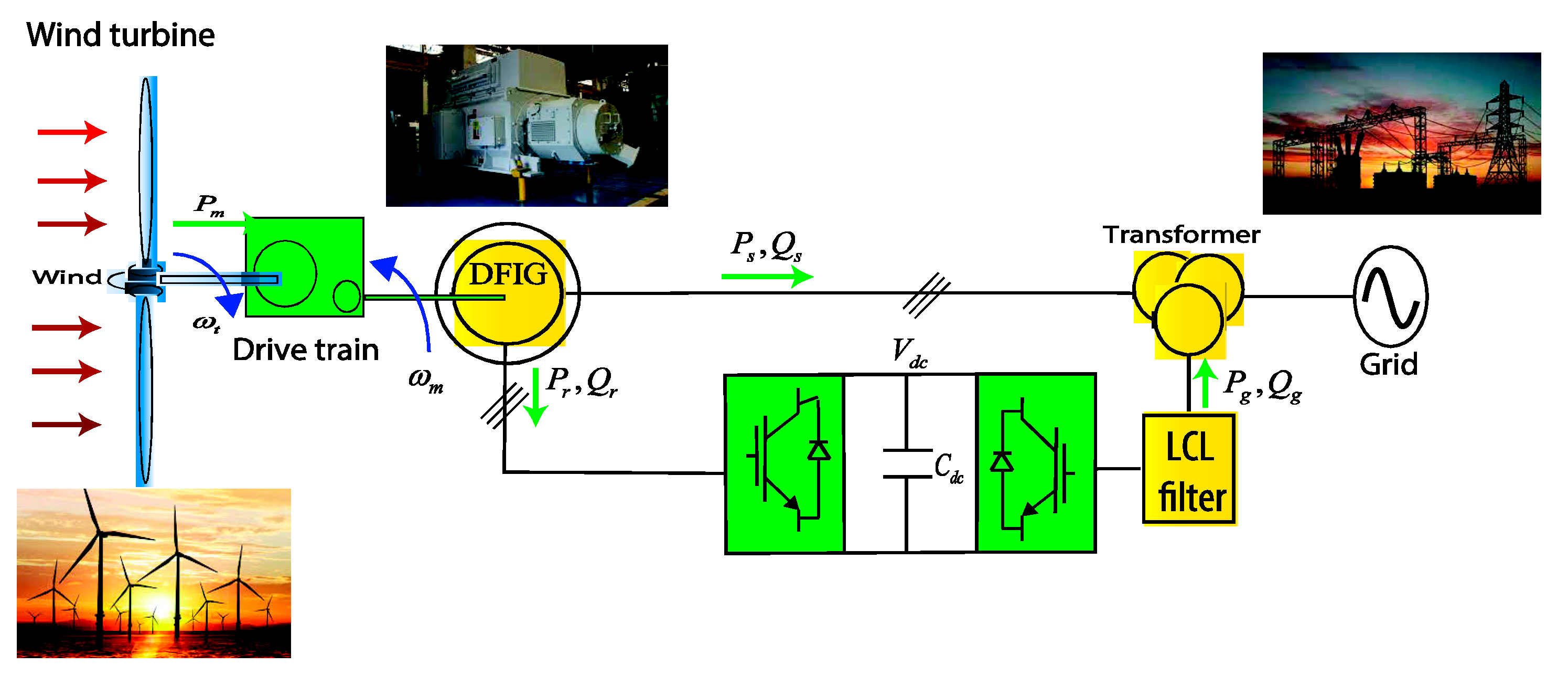
The configuration of the DFIG-based WECS is depicted in Figure 1. A WT is joined to the DFIG by means of a gearbox. The DFIG is an induction machine, which the stator windings are directly connected to the grid, while the rotor windings are connected to the grid thanks to a back-to-back converter.

2.1. Modelling of the Wind Turbine

The rotor blade of the WT is responsible for catching the wind power and converting it into kinetic energy. The captured mechanical power $P_m$ is given as follows [2]:

$$P_m=\frac{1}{2}\rho C_p\left(\lambda ,\beta \right)\pi R^2{V}_w^3$$

(1)

where $\rho$ is the air density, $C_p$ is the power coefficient and it depends on both the tip-speed ratio $\lambda$ and the blade pitch angle $\beta$, $R$ is the turbine radius and $V_w$ is the wind speed.

The tip speed ratio is defined as the ratio of the blade tip speed to the wind speed. It is given by:

$$\lambda =\frac{{\mathsf{\Omega }}_{t}R}{V_w}$$

(2)

where ${\mathsf{\Omega }}_t$ is the angular speed of the WT.

2.2. Modelling of the DFIG

The dynamical model of the studied DFIG can be expressed by the following electrical equations [6,7,8]:

$$\{\begin{array}{l}{V}_{ds}=R_s{i}_{ds}+\frac{d{\phi }_{ds}}{dt}-{\omega }_s{\phi }_{qs}\hfill \\ V_{qs}=R_s{i}_{qs}+\frac{d{\phi }_{qs}}{dt}+{\omega }_s{\phi }_{ds}\hfill \\ V_{dr}=R_r{i}_{dr}+\frac{d{\phi }_{dr}}{dt}-({\omega }_s-{\omega }_m){\phi }_{qr}\hfill \\ V_{qr}=R_r{i}_{qr}+\frac{d{\phi }_{qr}}{dt}+({\omega }_s-{\omega }_m){\phi }_{dr}\hfill \end{array}$$

(3)

where $V_s$ and $i_s$ are the stator voltage and current, $V_r$ and $i_r$ are the rotor voltage and current, ${\phi }_s$ and ${\phi }_r$ are the stator and rotor flux linkages, $R_s$ and $R_r$ are the stator and rotor resistances, ${\omega }_s$ and ${\omega }_m$ are the stator and rotor angular frequencies, respectively. The subscripts $d$ and $q$ denote the direct and quadrature axis components, respectively. The stator and rotor flux linkages are defined as follows:

$$\{\begin{array}{l}{\phi }_{ds}=L_s{i}_{ds}+L_m{i}_{dr}\mathrm{and}{\phi }_{qs}=L_s{i}_{qs}+L_m{i}_{qr}\\ {\phi }_{dr}=L_r{i}_{dr}+L_m{i}_{ds}\mathrm{and}{\phi }_{qr}=L_r{i}_{qr}+L_m{i}_{qs}\end{array}$$

(4)

where $L_s$, $L_r$ and $L_m$ are the stator, rotor and magnetizing inductances, respectively.

2.3. Modelling of the GSC and the DC-Link

The GSC is connected to the grid through an LCL-filter. However, for better understanding the control of GSC, it is necessary to describe the model of the grid side system and DC-link parts. The mathematical formulation of the GSC in the dq synchronous frame is defined by Equation (5). In this equation, $L_T$ represents the sum of the converter $L_i$ and grid side $L_g$ inductances. In fact, the LCL-filter can be approximated to an L-filter equal to the sum of the LCL-filter inductors [4]:

$$\{\begin{array}{l}{L}_T\frac{d{i}_{gd}}{dt}=-R_T{i}_{gd}+{\omega }_g{L}_T{i}_{gq}+e_{gd}-V_{df}\\ L_T\frac{d{i}_{gq}}{dt}=-R_T{i}_{gq}-{\omega }_g{L}_T{i}_{gd}+e_{gq}-V_{qf}\end{array}$$

(5)

where $V_{df}$ and $V_{qf}$ are the components of the converter side voltage, $i_{gd}$ and $i_{gq}$ are the components of the grid currents, $e_{gd}$ and $e_{gq}$ are the components of the grid voltage, and $R_T$ is the sum of the converter and grid side resistors.

The grid active and reactive powers are expressed as [9]:

$$\{\begin{array}{l}{P}_g=\frac{3}{2}\left(e_{dg}{i}_{dg}+e_{qg}{i}_{qg}\right)\hfill \\ Q_g=\frac{3}{2}\left(e_{qg}{i}_{dg}-e_{dg}{i}_{qg}\right)\hfill \end{array}$$

(6)

3. Vector Control of the DFIG-Based Wind Energy Converter

The classical direct power control of the DFIG system is divided into the RSC and GSC control loops, where the control structure for the RSC and GSC components consist of two cascaded control layers. The inner PI layers are adopted to regulate the components of rotor and grid currents. On the other hand, the outer PI ones in the RSC are implemented to control the active and reactive powers while the outer PI loop in the GSC is adopted to maintain the DC-link voltage to its reference value. However, in this work, the inner PI loops in the RSC and GSC circuits are designed based on a pole assignment technique [8,15], while the outer PI ones are tuned based on the proposed metaheuristics algorithms-based approach.

3.1. Control of the RSC

The RSC circuit is responsible to independently regulate the active and reactive powers in order to extract the maximum available power. The vector control by the SFO scheme is employed for the power regulation of the DFIG system.

Considering that the electrical network is stable, the stator flux ${\phi }_s$ is constant. In addition, for the medium and high power DFIG, the value of the stator resistance is very small and therefore it can be neglected [6,7]. Hence, based on these assumptions, the stator voltages and fluxes in Equation (3) and Equation (4) can be rewritten respectively as follows:

$$\{\begin{array}{l}{V}_{ds}=0\\ V_{qs}=V_s={\omega }_s{\phi }_{ds}\end{array}$$

(7)

$$\{\begin{array}{l}{\phi }_{ds}={\phi }_{ds}=L_s{i}_{ds}+L_m{i}_{dr}\\ {\phi }_{qs}=0=L_r{i}_{qs}+L_m{i}_{qr}\end{array}$$

(8)

The active and reactive stator powers and rotor voltages are given, respectively, by:

$$\{\begin{array}{l}{P}_s=\frac{3}{2}\left(V_{ds}{i}_{ds}+V_{qs}{i}_{qs}\right)=-\frac{3}{2}\frac{L_m}{L_s}{V}_s{i}_{qr}\hfill \\ Q_s=\frac{3}{2}\left(V_{qs}{i}_{ds}+V_{ds}{i}_{qs}\right)=\frac{3}{2}\left(\frac{V_s^2}{{\omega }_s{L}_s}-\frac{L_m}{L_s}{V}_s{i}_{dr}\right)\hfill \end{array}$$

(9)

$$\{\begin{array}{l}{V}_{dr}=R_r{i}_{dr}+\sigma L_r\frac{d{i}_{dr}}{dt}-\stackrel{{\Delta }_{dr}}{\overbrace{\sigma {\omega }_r{L}_r{i}_{qr}}}\hfill \\ V_{qr}=R_r{i}_{qr}+\sigma L_r\frac{d{i}_{qr}}{dt}+\stackrel{{\Delta }_{qr}}{\overbrace{\sigma {\omega }_r{L}_r{i}_{dr}+\frac{L_m}{L_s}{\omega }_r{\phi }_{ds}}}\hfill \end{array}$$

(10)

where $\sigma =L_r-L_m^2/L_s$ is the machine leakage coefficient and ${\omega }_r={\omega }_s-{\omega }_m$ is the slip angular frequency.

As shown in Equation (9), the stator active and reactive powers are independent from each other. In addition, the components of stator power are linearly varying with the direct and quadrature rotor currents. This powers’ regulation is thus performed using PI controllers for the d and q axis components of the rotor currents.

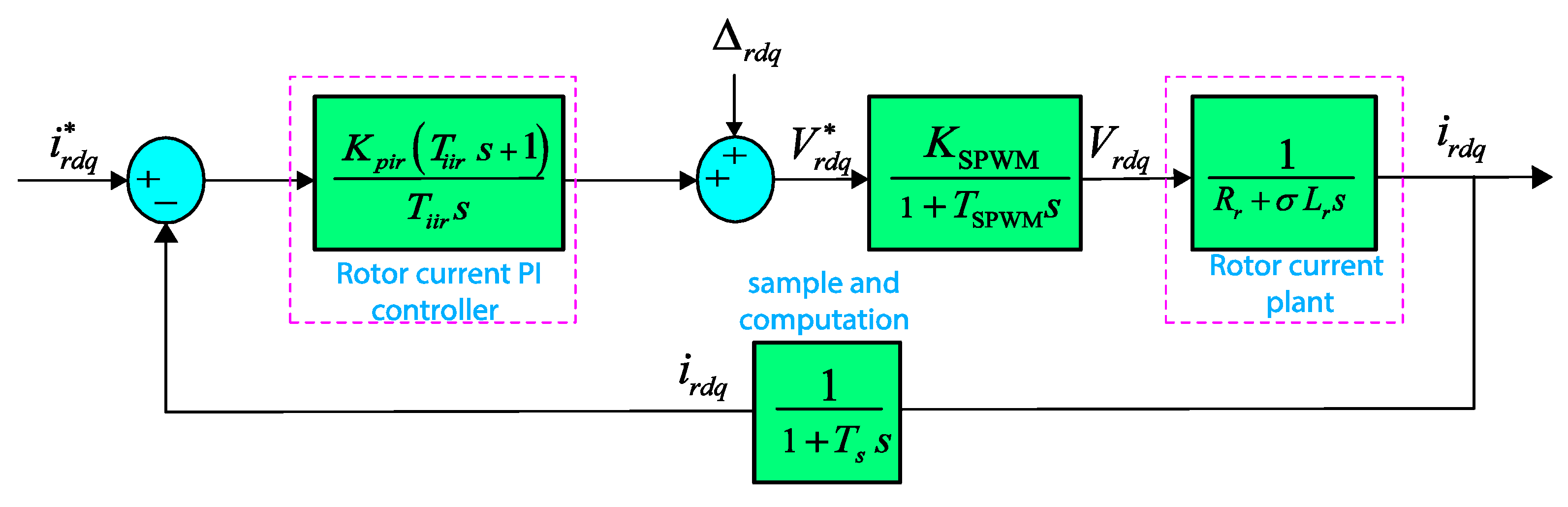
The outer control loops for the stator active and reactive powers are tuned based on the proposed metaheuristics-based procedure. Hence, the design of PI controllers for the inner rotor current loops is detailed according to Figure 2.

Based on a pole placement method as follows:

$$R_{PI}\left(s\right)=K_{pir}\left(1+\frac{1}{T_{iir}s}\right)$$

(11)

where $K_{pir}$ and $T_{iir}$ are the proportional gain and time constant of the rotor PI controllers, respectively.

The transfer function that describes the relationship between the voltages and currents dynamics is given as follows [8,15]:

$$R_{\mathrm{plant}}\left(s\right)=\frac{i_{rdq}}{V_{rdq}}=\frac{1}{R_r+\sigma L_{r}s}$$

(12)

Since the same transfer functions for the direct and quadrature rotor currents are considered, the closed-loop transfer function $R_{cli}\left(s\right)$ between the reference rotor current $i_{rdq}^{\ast }$ and the actual one $i_{rdq}$ is written as:

$$R_{cli}\left(s\right)=\frac{i_{rdq}}{i_{rdq}^{\ast }}=\frac{K_{pir}\left(T_{iir}s+1\right)}{T_{iir}\sigma L_r{s}^2+T_{iir}\left(R_r+K_{pir}\right)s+K_{pir}}$$

(13)

By equating the denominator of the closed-loop transfer function of Equation (13) under the general form of a second order system, the parameters of PI rotor current controllers can be found as follows [8,15]:

$$\{\begin{array}{l}{K}_{pir}=2\xi {\omega }_n\sigma L_r-R_r\\ T_{iir}=\frac{2\xi }{{\omega }_n}-\frac{R_r}{\sigma {\omega }_n{}^2{L}_r}\end{array}$$

(14)

where $\xi$ and ${\omega }_n$ are the damping coefficient and natural frequency of the desired closed-loop reference model, respectively.

For the design purpose, the discussion is made with respect to the choice of the damping coefficient $\xi$ and natural frequency ${\omega }_n$. Since the inner current loop in the cascade control scheme will have a much larger bandwidth than the one used in the outer-loop, a regulation at $1/20$ of the switching frequency $f_{sw,RSC}$ is retained. For the outer loop, a regulation between $1/20$ and $1/10$ of the inner loop bandwidth is made [5]. Then, feed forward compensations ${\Delta }_{dr}$ and ${\Delta }_{qr}$ should be added back to generate the desired rotor voltages $V_{dr}^{\ast }$ and $V_{qr}^{\ast }$.

3.2. Control of the GSC

The VOC strategy is applied to control the GSC, which usually contains one outer PI control loop that regulates the DC-link voltage regardless of the magnitude and the direction of the rotor power. Two inner PI current loops that regulate the direct and quadrature gird currents are also included [16,17]. In addition, the passive damping strategy is employed to mitigate the resonance problem. The mathematical representation of GSC is built on the approximated model of the LCL-filter, which is used to tune the PI grid current controllers. Whereas, the whole transfer function of the LCL-filter with passive damping is taken into account for the stability analysis and investigation [4]. The block diagram of the grid current loops is shown in Figure 3.

To implement the VOC scheme, the d-axis is aligned with the grid vector voltage. Therefore, this leads to a d-axis grid voltage equal to its magnitude, and the q-axis voltage which is then equal to zero. Hence, the grid power expressions can be expressed as [16,17]:

$$\{\begin{array}{l}{P}_g=\frac{3}{2}{e}_{dg}{i}_{dg}\\ Q_g=-\frac{3}{2}{e}_{dg}{i}_{qg}\end{array}$$

(15)

Equation (15) decides the active power and consequently the DC-link voltage is controlled via the direct current whereas the quadrature current is used to regulate the reactive power that exchanges with the grid [17]. With the VOC approach, the dynamic equations of the grid currents are rewritten as follows:

$$\begin{array}{l}{e}_{dg}=R_T{i}_{dg}-\stackrel{{\Delta }_{dg}}{\overbrace{{\omega }_g{L}_T{i}_{qg}}}+L_T\frac{d{i}_{dg}}{dt}+V_{df}\\ 0=R_T{i}_{qg}+\stackrel{{\Delta }_{qg}}{\overbrace{{\omega }_g{L}_T{i}_{dg}}}+L_T\frac{d{i}_{qg}}{dt}+V_{qf}\end{array}$$

(16)

By applying the same methodology of PI rotor current controllers design in the RSC, the gains of PI controllers for the grid currents dynamics are found as [15,18]:

$$\{\begin{array}{l}{K}_{pig}=2\xi {\omega }_n{L}_T-R_T\\ K_{iig}={\omega }_n^2{L}_T\end{array}$$

(17)

where ${\omega }_n=847.80\mathrm{rad}/\sec$ and $\xi =0.707$.

4. PI Controllers Tuning Problem Formulation

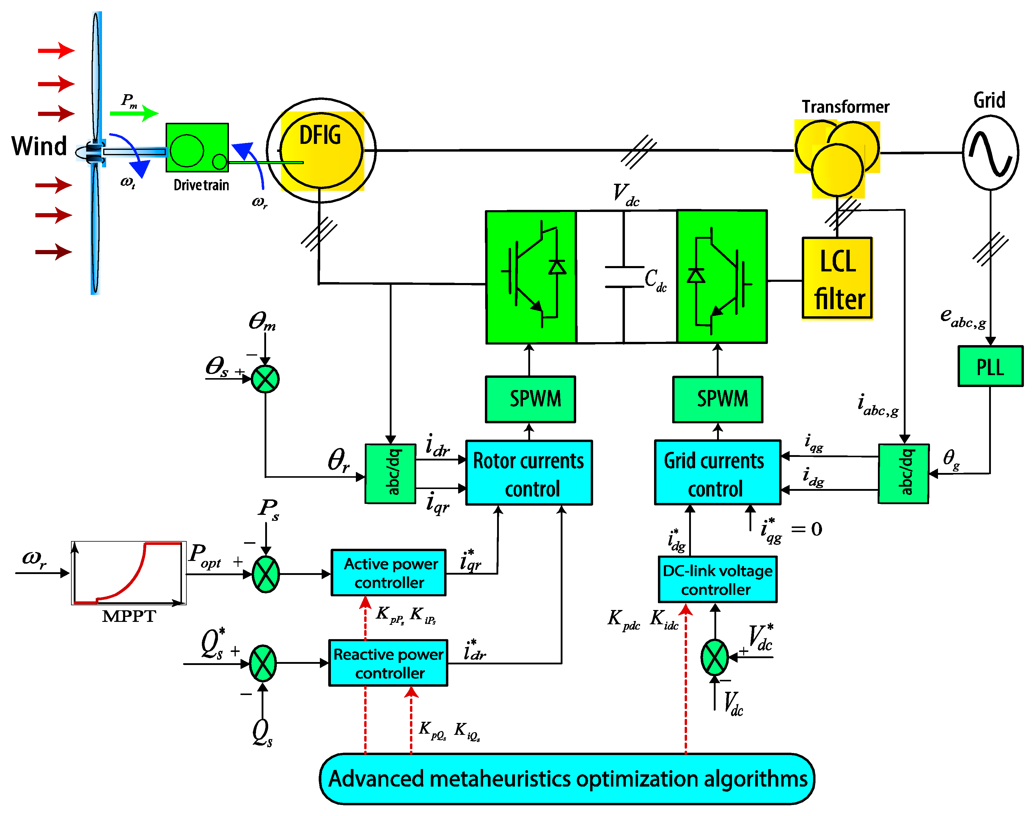
In the PI control framework, appropriate values of $K_p$ and $K_i$ gains are generally obtained by empirical methods and trials-errors based procedures [19]. These nonsystematic and challenging tasks become more difficult and time-consuming, especially for the complex and large-scale systems like the studied DFIG-based WECS. So, the idea of formulating the $K_p$ and $K_i$ gains’ selection as an optimization problem is a promising solution. Such a control problem can be nonlinear, non-smooth or even non-convex and can be effectively solved thanks to advanced metaheuristics [10,11]. In this work, three PI controllers for the outer-loops at both RSC and GSC components are considered for the optimization process. These PI controllers for the DC-link voltage, active and reactive powers’ dynamics are systematically tuned thanks to the proposed TEO metaheuristic which is described in the following. Figure 4 gives the proposed optimization-based tuning scheme of the PI controllers for the DFIG-based WECS.

The decision variables of the formulated optimization problem are obviously the proportional and integral gains of PI controllers for the active/reactive powers and DC-link loops. They are specified for the optimization process as follows:

$$\mathit{x}={\left[K_{p{P}_s},K_{i{P}_s},K_{p{Q}_s},K_{i{Q}_s},K_{pdc},K_{idc}\right]}^T\in \mathcal{S}\subseteq {\mathbb{R}}_{+}^6$$

(18)

where $\mathcal{S}=\{\mathit{x}\in {\mathbb{R}}_{+}^6,{\mathit{x}}_{low}\le \mathit{x}\le {\mathit{x}}_{up}\}$ denotes the bounded search space for all PI parameters.

However, the defined objective functions are minimized taking into account a scope of time-domain restrictions. These are concerning to the maximum overshoot ${\delta }^{\max }$, steady-state error $E_{ss}$, rise time $t_r$ and/or settling time $t_s$ of the closed-loop system step-response [20]. So, the tuning issue associating the PI controllers of the DFGI-based WECS can be expressed as follows:

$$\{\begin{array}{l}\mathrm{Minimize}{f}_m\left(\mathit{x}\right),m\in \{IAE,ISE,ITSE,ITAE\}\\ \mathit{x}={\left[K_{p{P}_s},K_{i{P}_s},K_{p{Q}_s},K_{i{Q}_s},K_{pdc},K_{idc}\right]}^T\in \mathcal{S}\subseteq {\mathbb{R}}_{+}^6\\ \mathrm{subject}\mathrm{to}:\\ g_1\left(\mathit{x}\right)={\delta }_{P_s}-{\delta }_{P_s}^{\max }\le 0\\ g_2\left(\mathit{x}\right)={\delta }_{Q_s}-{\delta }_{Q_s}^{\max }\le 0\\ g_3\left(\mathit{x}\right)={\delta }_{dc}-{\delta }_{dc}^{\max }\le 0\\ K_{pj,\min }\le K_p\le K_{pj,\max }\\ K_{ij,\min }\le K_i\le K_{ij,\max },j\in \left\{P_s,Q_s,dc\right\}\end{array}$$

(19)

where $f_m:{\mathbb{R}}_{+}^6\to \mathbb{R}$ are the cost functions, $g_q:{\mathbb{R}}_{+}^6\to \mathbb{R}$ are the problem’s inequality constraints, ${\delta }_{dc}$, ${\delta }_{P_s}$ and ${\delta }_{Q_s}$ are the overshoots of the controlled DC-voltage, active and reactive powers dynamics, respectively, ${\delta }_{dc}^{\max }$, ${\delta }_{P_s}^{\max }$ and ${\delta }_{Q_s}^{\max }$ denote their maximum given value.

Since the optimization problem (19) is a multi-objective type, weighted sum-based aggregation functions are used as follows to handle with the multiple costs [21]:

$$f_{IAE}\left(\mathit{x}\right)=w_{P_s}{\displaystyle {\int }_0^T\left|e_{P_s}\left(\mathit{x},t\right)\right|dt}+w_{Q_s}{\displaystyle {\int }_0^T\left|e_{Q_s}\left(\mathit{x},t\right)\right|dt}+w_{dc}{\displaystyle {\int }_0^T\left|e_{dc}\left(\mathit{x},t\right)\right|dt}$$

(20)

$$f_{ISE}\left(\mathit{x}\right)=w_{P_s}{\displaystyle {\int }_0^T{e}_{P_s}^2\left(\mathit{x},t\right)dt}+w_{Q_s}{\displaystyle {\int }_0^T{e}_{Q_s}^2\left(\mathit{x},t\right)dt}+w_{dc}{\displaystyle {\int }_0^T{e}_{dc}^2\left(\mathit{x},t\right)dt}$$

(21)

$$f_{ITSE}\left(\mathit{x}\right)=w_{P_s}{\displaystyle {\int }_0^{T}t{e}_{P_s}^2\left(\mathit{x},t\right)dt}+w_{Q_s}{\displaystyle {\int }_0^{T}t{e}_{Q_s}^2\left(\mathit{x},t\right)dt}+w_{dc}{\displaystyle {\int }_0^{T}t{e}_{dc}^2\left(\mathit{x},t\right)dt}$$

(22)

$$f_{ITAE}\left(\mathit{x}\right)=w_{P_s}{\displaystyle {\int }_0^{T}t\left|e_{{}_{P_s}}\left(\mathit{x},t\right)\right|dt}+w_{Q_s}{\displaystyle {\int }_0^{T}t\left|e_{Q_s}\left(\mathit{x},t\right)\right|dt}+w_{dc}{\displaystyle {\int }_0^{T}t\left|e_{dc}\left(\mathit{x},t\right)\right|dt}$$

(23)

where $T$ denotes the total simulation time, $w_{P_s}>0$, $w_{Q_s}>0$ and $w_{dc}>0$ are the weighting coefficients of the aggregation functions satisfying $w_{P_s}+w_{Q_s}+w_{dc}=1$, and $e_j(.),j\in \left\{P_s,Q_s,dc\right\}$ denote the tracking errors between the plant output and the relative set-point values, i.e., $e_{P_s}\left(\mathit{x},t\right)=P_s^{*}-P_s\left(\mathit{x},t\right)$, $e_{Q_s}\left(\mathit{x},t\right)=Q_s^{*}-Q_s\left(\mathit{x},t\right)$ and $e_{dc}\left(\mathit{x},t\right)=V_{dc}^{\ast }-V_{dc}\left(\mathit{x},t\right)$.

The judgment matrix method is used to determine the weighting coefficients of the objective functions [22,23]. Such a method grades all objective functions based on the importance of each one. After calculating the eigenvalues of such a matrix, the weighting coefficients of functions (20)–(23) can be chosen as $w_{P_s}=0.6370$, $w_{Q_s}=0.2583$ and $w_{dc}=0.1047$.

5. Thermal Exchange Optimization Algorithm

The Thermal Exchange Optimization (TEO) algorithm is a novel metaheuristic inspired by Newton’s law of the cooling [3]. In this population-based metaheuristic, each agent is modeled as a cooling object. By associating another agent as a surrounding fluid, a heat transfer and thermal exchange occurs between them. The new temperature of each agent is considered as a new position of the potential solution in the search space.

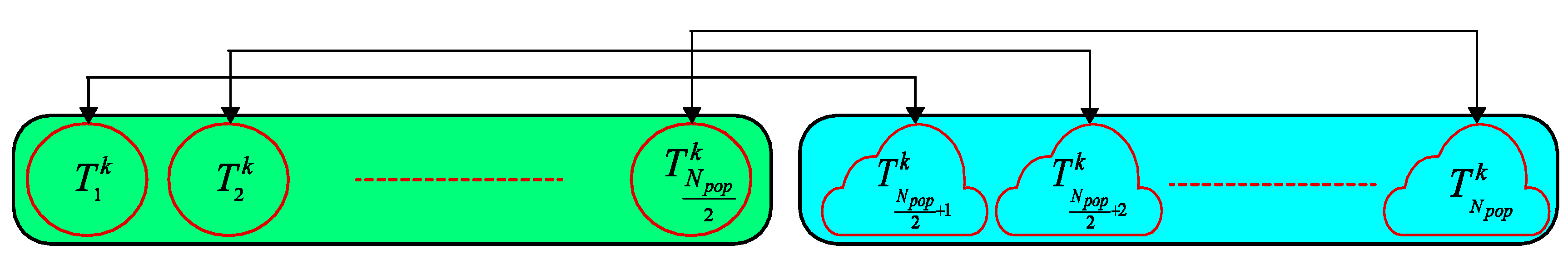
In a d-dimensional search space and at the $k^{th}$ iteration time, each object of the population is described by its temperature ${\mathit{T}}_i^k=\left(T_{i,1}^k,T_{i,2}^k,\dots ,T_{i,d}^k\right)$, $\left(i,k\right)\in \left[1,N_{pop}\right]\times \left[0,N_{iter}\right]$. In order to enhance the optimization performances, the TEO algorithm uses a Thermal Memory (TM) to store a number of historically best vectors as well as their related fitness. Therefore, these stored solution vectors are added to the population and the same numbers of current worst objects are deleted. After that, a growing order of solutions is retained according to their cost function values. The $N_{pop}$ sorted objects are equally divided into two groups of environment and cooling objects as shown in Figure 5. The environment objects are denoted as $T_{{}_1}^k,T_{{}_2}^k,\dots ,T_{N_{pop}/2}^k$ while the cooling ones are $T_{{N_{pop}/2}_{+1}}^k,T_{{N_{pop}/2}_{+2}}^k,\dots ,T_{{}_{N_{pop}}}^k$.

Since the object has lower $\eta$ can exchange the temperature slightly, the TEO metaheuristic proposed a similar formula to evaluate the value of $\eta$ for each object as described in Equation (24):

$$\eta =\frac{\mathrm{Cost}\left(\mathrm{object}\right)}{\mathrm{Cost}(\mathrm{worst}\mathrm{object})}$$

(24)

Over the course of iterations, the value $t=k/N_{iter}$ increases as follows leading to improving the exploration mechanism [3]. In order to enhance the TEO exploration capacity, Equation (25) has been proposed to avoid the trapping in local optima and update the environmental temperature as follows:

$$T_{env,i}^{k+1}=\left(1-\mathcal{U}\left\{0,1\right\}\left(c_1+c_2\left(1-t\right)\right)\right)T_{env,i}^k$$

(25)

where $c_1$ and $c_2$ are the controlling variables chosen as 0 or 1, $\mathcal{U}\left\{0,1\right\}$ is a uniformly random number, $T_{env,i}^k$ is the previous environmental temperature, $\left(1-t\right)$ is proposed to reduce the randomness by closing to the last iterations. When the decreasing of the randomness is not required, the value of $c_2$ is set to zero.

The new temperatures for each object, i.e., either cooling objects or environmental ones, are updated as follows:

$$T_i^{k+1}=T_{env,i}^k+\left(T_i^k-T_{env,i}^k\right)e^{-\eta t}$$

(26)

In the TEO formalism, another formulation is suggested to improve the exploration ability. A control parameter $0\le pro\le 1$ is introduced and determines whether a component of each cooling object must be changed or not. For each object, such a parameter is compared to $Rand\left(i\right),\left(i=1,2,\dots ,N_{pop}\right)$, which is a random number uniformly distributed between 0 and 1. If $Rand\left(i\right)<pro$, one dimension of the $i^{th}$ object is chosen randomly and its value is regenerated as follows [3,24]:

$$T_{\left(i,j\right)}=T_{j,\min }+\mathcal{U}\left(0,1\right)\times \left(T_{j,\max }-T_{j,\min }\right)$$

(27)

where $T_{\left(i,j\right)}$ is the $j^{th}$ component of the $i^{th}$ object, $T_{j,\max }$ and $T_{j,\min }$ are the upper and lower bounds of the $j^{th}$ component, respectively.

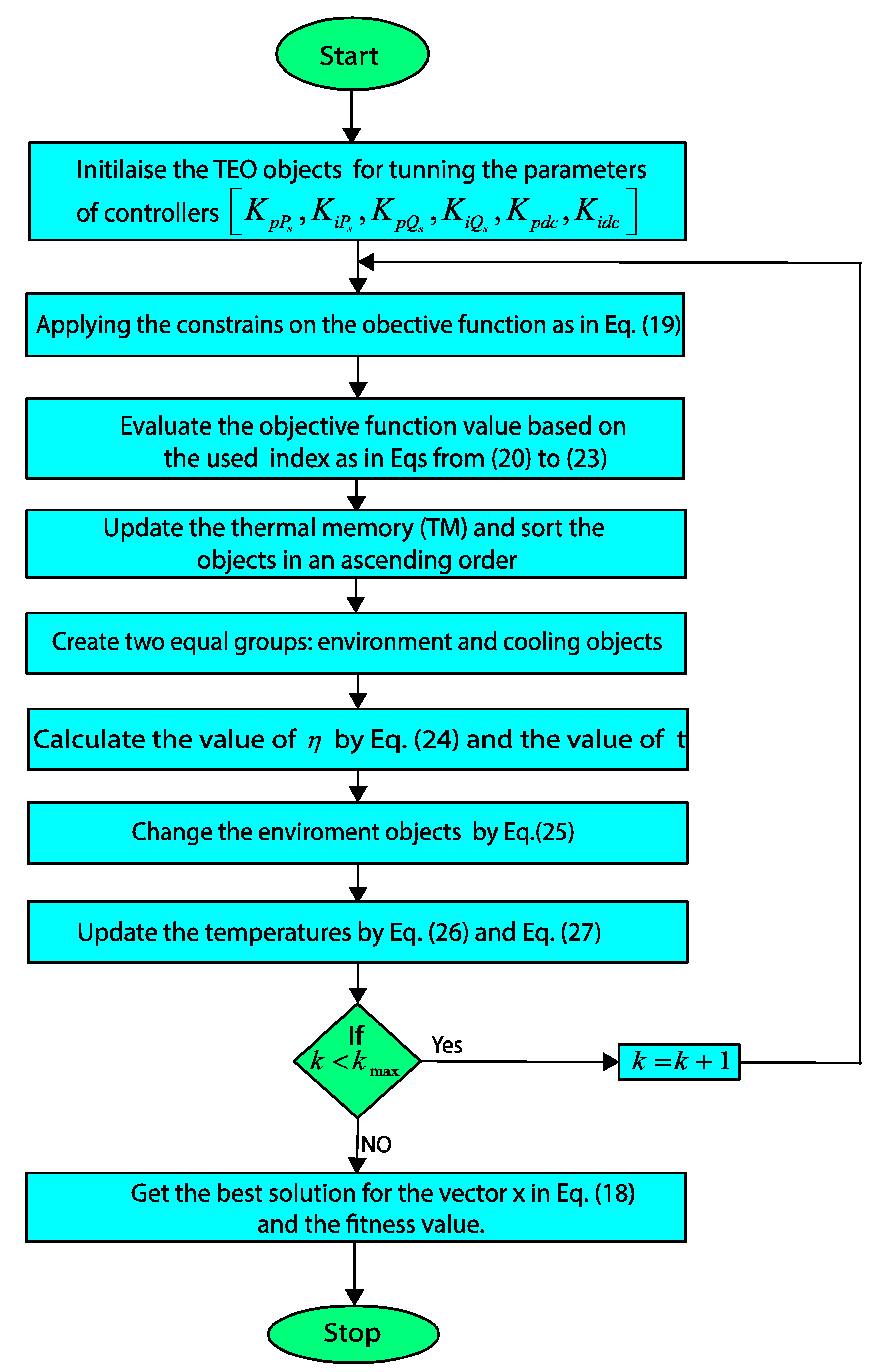
Finally, the steps of the proposed TEO algorithm are summarized as follows:

• Step 1. Randomly initialize the temperature for all objects $T_i^0$, $i=1,2,\dots ,N_{pop}$.
• Step 2. Calculate the fitness of each search object.
• Step 3. Save some $T$ best vectors and their related cost values in the TM.
• Step 4. Add the saved solutions and remove the same numbers of the worst objects.
• Step 5. Arrange the objects according to their related fitness in an ascending order.
• Step 6. Divide the objects into two equal groups: environment and cooling objects.
• Step 7. Calculate the parameters $\eta$ and $t$.
• Step 8. Change the environment temperatures by Equation (25).
• Step 9. Update the temperatures according to Equations (26) and (27).
• Step 10. Check the termination criterion and repeat the iterations.

To describe the proposed metaheuristics-based tuning strategy of the PI controllers in the studied DFIG-based energy conversion system, a detailed flowchart is shown in Figure 6.

6. Simulation Results and Discussions

6.1. Execution of the Metaheuristic Algorithms

The proposed metaheuristics-based direct power control of the studied DFIG-based WECS is built using the MATLAB/Simulink environment. The respective nominal parameters of the DFIG, power converters at both sides, L-filter and LCL-filter are presented in

Table 1. Parameters for a 1.5 MW DFIG systems.

Equipment	Parameter	Value	Unit
DFIG	Rated power	1500	kW
	RMS grid line voltage	575	V
	Slip range	0.2	-
	Rated electrical frequency	50	Hz
	Stator resistance	0.023	pu
	Stator leakage inductance	0.18	pu
	Rotor resistance	0.016	pu
	Rotor leakage inductance	0.16	pu
	Magnetizing inductance	2.9	pu
Power converters	Rated power	300	kW
	Switching frequency at $f_{sw,RSC}$ and $f_{sw,GSC}$	2700	Hz
	DC-link voltage	1050	V
	DC-link capacitance	10000	$\mathsf{\mu }\mathrm{F}$
L-filter	L-filter grid inductance	0.1	pu
LCL-filter	LCL-filter grid side inductance	0.018	pu
	LCL-filter capacitance	0.104	pu
	LCL-filter converter side inductance	0.077	pu
	Passive damping resistor	0.124	pu

. Specifically, this work deals with the PI controllers tuning for the active and reactive powers loops in the RSC circuit, as well as it treats with the PI controller optimization-based selection of the DC-link voltage loop in the GSC component. It is worth indicating that the inner current loops in the RSC and GSC are tuned according to the pole assignment method. Since the grid current closed-loop of the LCL-filter is unstable, the passive damping method is applied as a solution to ensure the stability of such current dynamics. To investigate the effectiveness and superiority of the proposed TEO method, the well-known global algorithms GA, PSO, HSA, WCA and GOA are considered for comparison purposes.

All reported algorithms are independently run 10 times. The termination criterion is set as a maximum number of iteration reached $N_{iter}=100$ for a population size of the thermal agents equal to $N_{pop}=50$. All the values of the used common parameters are kept equal. All algorithms have been executed on a PC computer with Core TM i5-7200U CPU and 2.5 GHz/8.00 GB RAM. The specific control parameters of the reported algorithms are listed in

Table 2. Parameter setting of reported algorithms.

Algorithms	Parameters Setting
PSO	Cognitive and social coeffs. $c_1=c_2=2$, weights $w_{\max }=0.9$, $w_{\min }=0.2$ [10].
GA	Roulette wheel, crossover ${\mathcal{P}}_{cross}=1$, mutation ${\mathcal{P}}_{mut}=0.01$ [11].
HSA	Harmony memory rate HMCR = 0.9, pitch adjusting rate PAR = 0.3 [25].
WCA	Summation number of rivers $N_{sr}=8$ and $d_{max}=1\times {10}^{-3}$ [18].
GOA	$c_{\max }=1$, $c_{\min }=0.00001$ [26].
TEO	Thermal memory $TM=10$, $pro=0.50$, $c_1=1,c_2=1$ [3].

.

The optimization problem (19) is minimized for various performance criteria, i.e., IAE, ISE, ITAE and Integral Time-weighted Square Error (ITSE), and under time-domain operational constraints. These performance indexes are calculated within two conditions, which are considered as follows:

-

14.3% step change in the reference of DC-link voltage at time $t=0.5\sec$;

-

step change in the reference stator reactive power at time $t=0.8\sec$.

To find the accurate values of the decision variables $\mathit{x}=\left[K_{p{P}_s},K_{i{P}_s},K_{p{Q}_s},K_{i{Q}_s},K_{pdc},K_{idc}\right]$, the bounded search domain is initially set to $0\le \mathit{x}\in {\mathbb{R}}_{+}^6\le {10}^5$. Several runs of the algorithm are performed within this initial limitation. The results indicated that the search space could be reduced to $0\le \mathit{x}\in {\mathbb{R}}_{+}^6\le 400$. Therefore, the TEO algorithm explores within a smaller search domain for the next runs and more precise solution output vector is achievable.

Table 3. Statistical results of optimization problem (19) over 10 independent runs.

Indices		PSO	GA	HSA	WCA	GOA	TEO
IAE	Best	1.57	1.62	1.57	1.52	1.60	1.55
	Mean	1.73	1.67	1.60	1.59	2.01	1.58
	Worst	2.69	1.73	1.64	1.78	3.20	1.60
	STD	3.4 × 10−1	3.2 × 10−2	2.3 × 10−2	7.6 × 10−2	6.3 × 10−1	1.9 × 10−2
	ET (sec)	29022	28720	25480	32900	20400	24640
ISE	Best	33.17	34.86	32.64	32.66	34.06	31.45
	Mean	41.42	37.25	35.51	45.88	45.06	33.46
	Worst	61.80	40.53	38.78	61.24	64.50	36.79
	STD	8.27	1.92	1.80	10.77	9.08	1.64
	ET (sec)	28140	27420	19083	26900	19200	23420
ITSE	Best	17.47	17.49	18.45	17.14	17.86	17.79
	Mean	18.46	17.96	23.18	18.32	19.83	18.24
	Worst	20.45	18.21	26.77	19.75	28.11	19.20
	STD	0.921	0.207	3.616	8.1E-1	2.96	4.1E-1
	ET (sec)	21560	26280	18720	27540	19500	23380
ITAE	Best	0.650	0.632	0.646	0.640	0.644	0.642
	Mean	0.683	0.650	0.683	0.659	0.688	0.658
	Worst	0.707	0.62	0.718	0.736	0.742	0.675
	STD	0.018	0.019	0.021	0.029	0.040	0.014
	ET (sec)	20060	20480	16880	25880	20840	19680

gives the statistical results attained by the introduced algorithms under minimizing the cost functions described in Equations (20)–(23). The worst, average, best values and the standard deviation (STD) experimental results are summarized in the Table 3, where the optimal mean value of each index is highlighted in bold and underlined. In addition, the Elapsed Time (ET) is also listed, which is defined as the time that any algorithm requires finding the best solution. It can be clearly observed that the proposed TEO produces very competitive solutions with the reported algorithms. Appendix A summarizes the obtained gains of the PI controllers for each proposed optimization method. Indeed, these tuned PI controllers’ gains lead to the best transient and steady state responses of the entire reported algorithms.

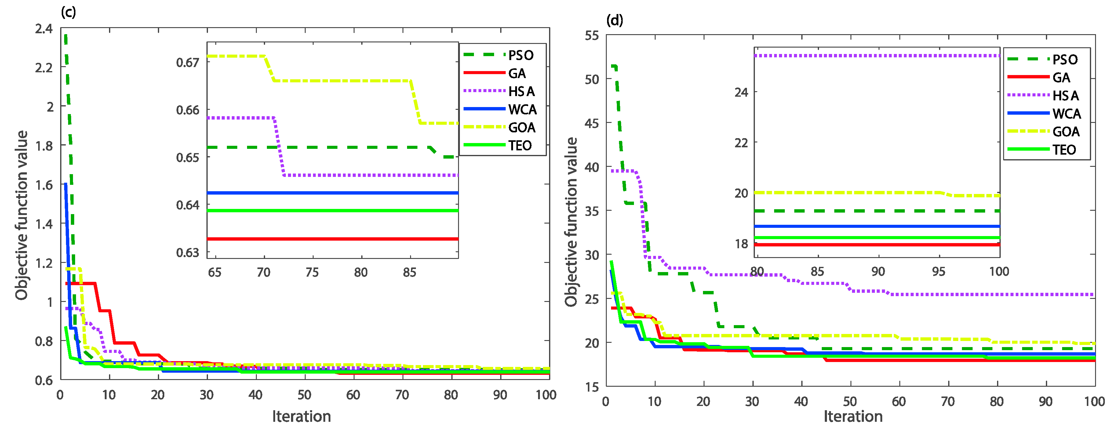
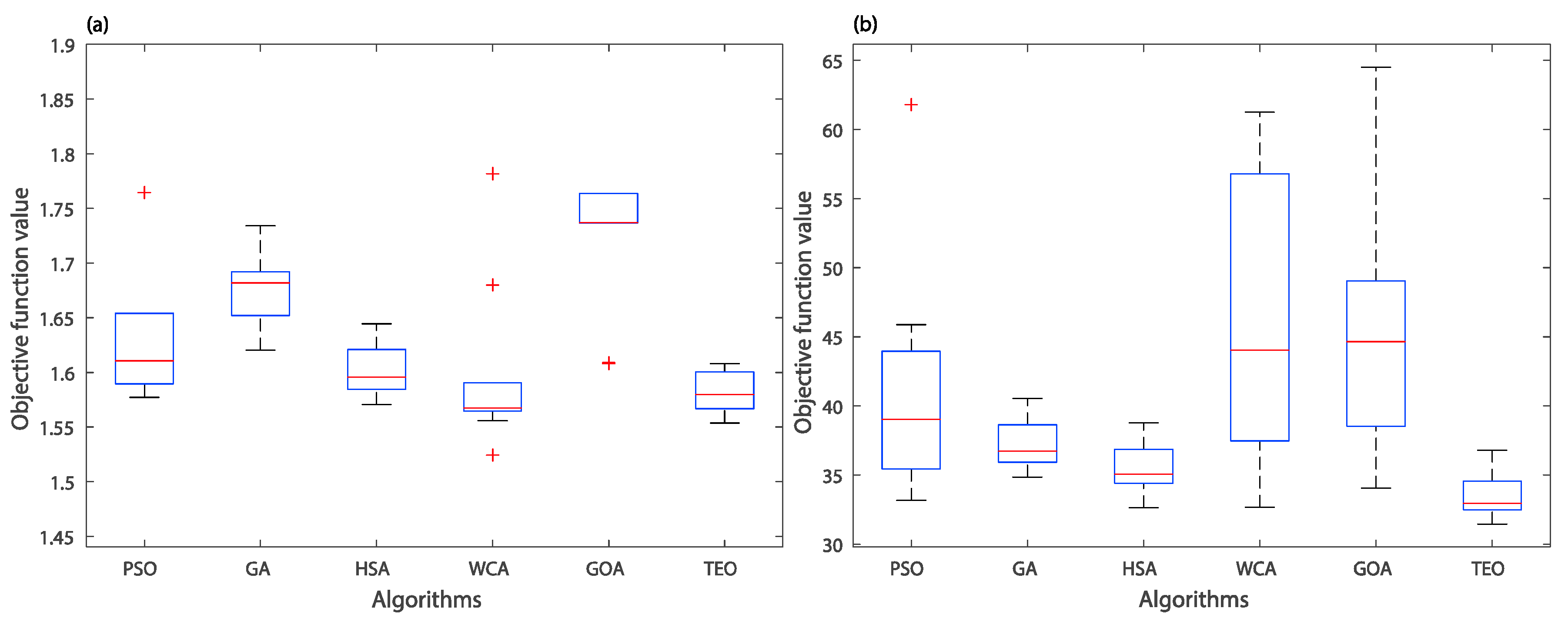
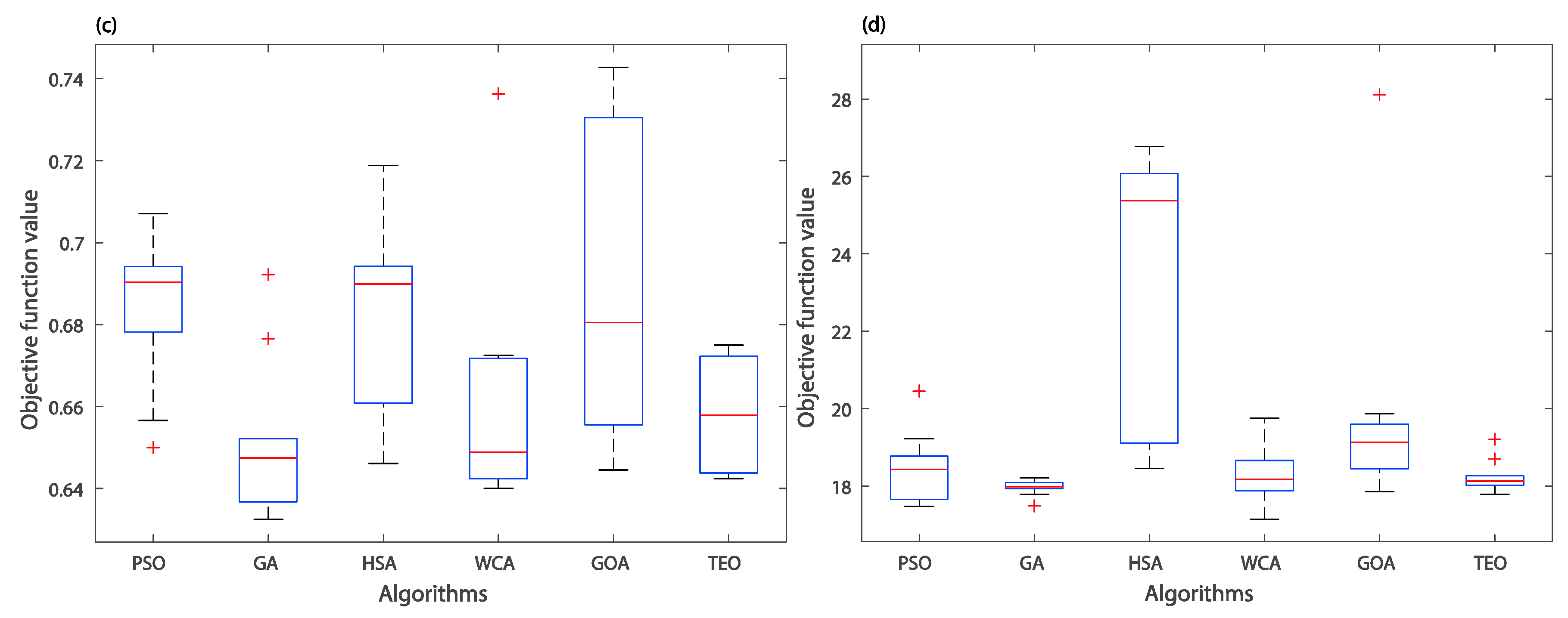
In addition, Figure 7 shows the convergence histories of the mean objective function values of IAE, ISE, ITAE and ITSE criteria, respectively. Indeed, it is shown that the proposed TEO metaheuristic for both IAE and ISE indices outperforms the other reported methods in terms of the fastness and non-premature convergence as well as the solutions’ quality. The TEO-based method for ITAE and ITSE criteria gives the best solution as a second order after the GA one. From these results, the superiority of the TEO metaheuristic is still shown in terms of exploitation and exploration capabilities for local and global searches. This further justifies the use of such a global metaheuristic to systematic and easy design of the direct power control of the DFIG-based WECS. The Box-and-Whisker plots of the mean objective function values are shown in Figure 8. From these results, one can observe that the boxplots of the TEO algorithm for all given performance criteria are generally lower and narrower than other algorithms. This confirms the high reproductivity of the TEO algorithm toward finding the optimal values of the solution.

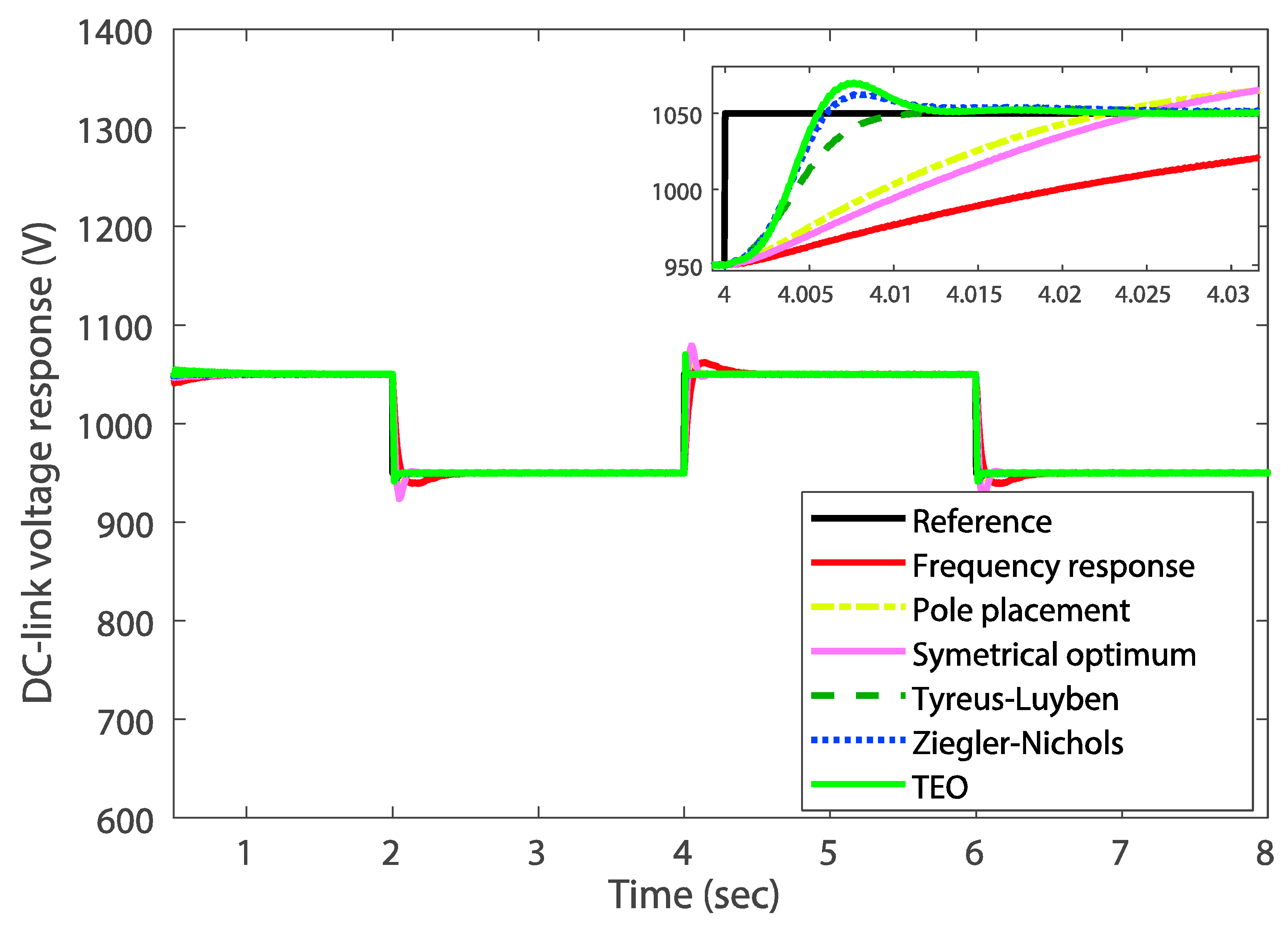
In the remainder of the results, the obtained gains of the optimized PI controllers are used to assess the frequency-and time-domains performances of the outer-loops at the RSC and GSC power components. Moreover, comparisons with the classical pole placement [8,15], frequency response [5] symmetrical optimum [27], Ziegler–Nichols [28] and Tyreus–Luyben [29] tuning methods are made for the DC-link voltage dynamics as shown in

Table 4. Time-domain performances for controlled DC-link voltage under step changes scenario.

PI Tuning Methods	Unit Step Change Response
	${\mathit{t}}_{\mathit{r}}\left(\mathbf{sec}\right)$	${\mathit{t}}_{\mathit{s}}\left(\mathbf{sec}\right)$	${\mathit{t}}_{\mathit{p}}\left(\mathbf{sec}\right)$	$\mathit{\delta }(\mathbf{\%})$	${\mathit{E}}_{\mathit{s}\mathit{s}}$
Frequency response	0.0441	4.3813	4.1382	1.168	0.3355
Pole placement	0.0163	4.1111	4.0441	2.006	0.2813
Symmetrical optimum	0.0185	4.1324	4.0459	2.768	0.3568
Ziegler–Nichols	0.0037	4.0252	4.0080	1.209	0.2843
Tyreus–Luyben	0.0060	4.0249	4.0182	0.299	0.2977
TEO	0.0029	4.0193	4.0076	2.537	0.2539

and Figure 9. The closed-loop response of the DC-link voltage dynamics is investigated under variable voltage profile. The DC-link voltage reference is varied up and down at various step levels. Figure 9 describes such a response around the final set-point value for different tuned PI controllers. Although, in real systems, the DC-link voltage is required to be constant. This scenario is proposed to check the capability of the proposed TEO algorithm under different circumstances. The aim is to show the difference between the classical tuning methods and the proposed optimization-based one. Referring to this result, the ITAE-based TEO algorithm can regulate the DC-link voltage dynamics with higher performance compared to the other algorithms.

The voltage tracking is achieved with best performance in terms of response precision and fastness, i.e., the steady-state error and rise/settling time metrics are minimal as depicted in Table 4. The performance in terms of response damping is acceptable for the proposed TEO-tuned PI control as shown in Figure 9. Referring to the numerical results in Table 4, one can clearly observe that the proposed TEO algorithm showed the best rise/settling times and steady-state error except the overshoot index, which the Tyreus–Luyben method gained the minimum overshoot. Since several runs were executed to obtain the PI controllers’ gains with the classical Ziegler–Nichols and Tyreus–Luyben methods, the tuning process becomes a tedious and time-consuming task. These minor degradations of the overshoot performance do not influence the effectiveness of the proposed TEO-based tuning method with respect to the systematization of the synthesis procedure, the simplicity of implementation and the superiority in other performance indices. The proposed TEO algorithm found the optimal gains of the PI controllers within a reduced computation time and under operational constraints compared to the reported trials-errors based tuning procedures which generally give local solutions for the formulated control problem.

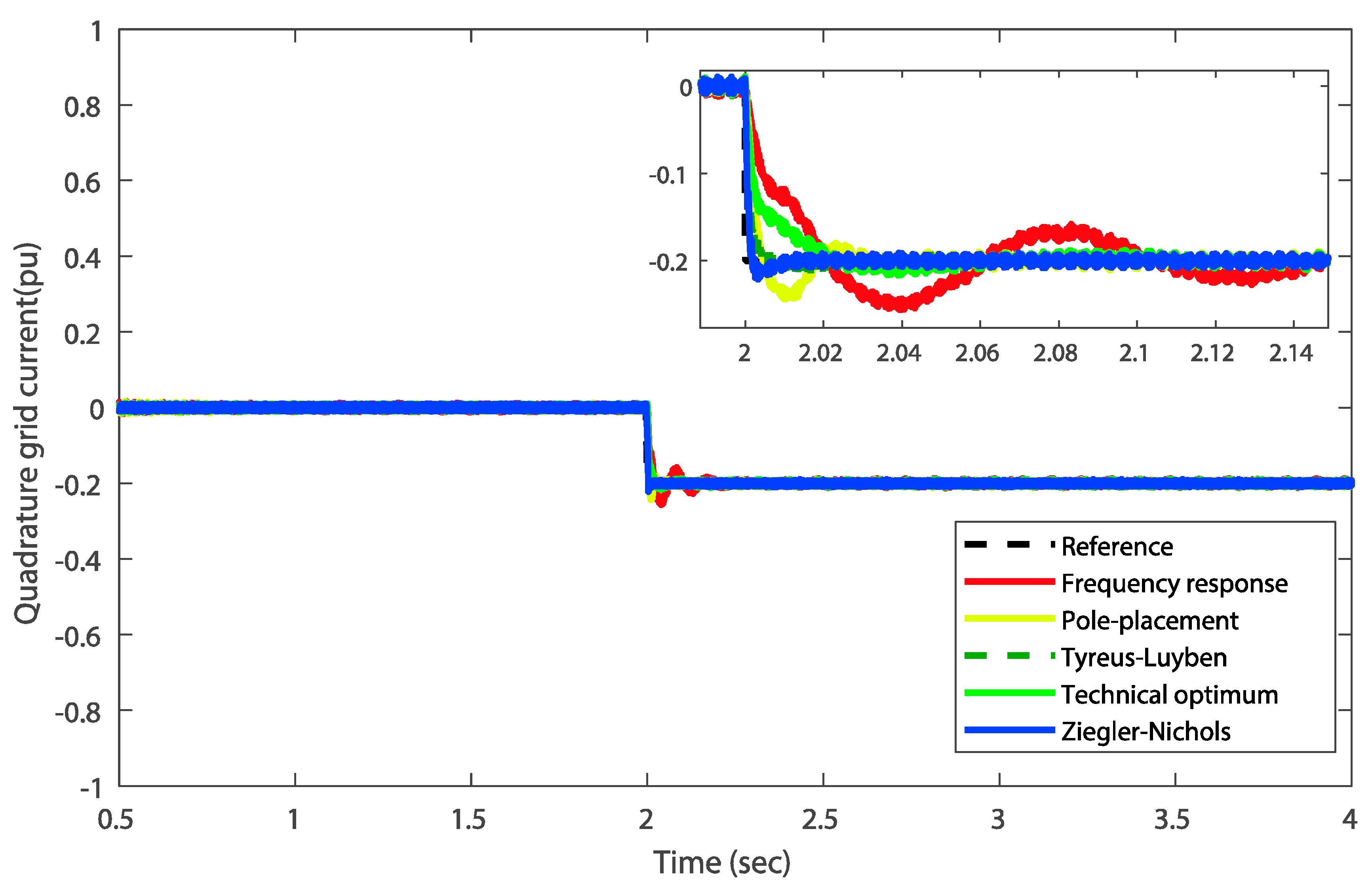
Regarding to the grid current dynamics, the same tuning methods with adding the technical optimum instead of the symmetrical ones are used to select and adjust the PI controllers’ gains. All obtained results are reported in

Table 5. Time-domain performances for controlled quadrature grid current under a step change scenario.

PI Tuning Methods	Unit Step Change Response
	${\mathit{t}}_{\mathit{r}}\left(\mathbf{sec}\right)$	${\mathit{t}}_{\mathit{p}}\left(\mathbf{sec}\right)$	$\mathit{\delta }(\mathbf{\%})$	${\mathit{E}}_{\mathit{s}\mathit{s}}$
Frequency response	0.0171	2.0387	28.1802	0.0035
Pole placement	0.0027	2.0096	21.95	0.0045
Technical optimum	0.0146	2.0383	8.2931	0.0055
Ziegler–Nichols	3.582 × 10−4	2.0026	10.7400	0.0051
Tyreus–Luyben	0.0020	2.0155	7.1657	0.0061

.

The control performance of the introduced tuning methods is investigated by supposing that there is a step change in the q-axis grid current reference at time $t=0.2\sec$. The reference q-axis grid current is changed from zero to −0.2 pu. However, the q-axis reference grid current is usually set at zero to achieve a unity power factor. Figure 10 shows the quadrature grid current response under step changes. It can be observed that the Tyreus–Luyben method gives superior performance in comparison with the other reported methods. Here, it is important to mention that the gains of the PI controllers for the inner current loops at both RSC and GSC are selected thanks to the classical methods and not with the proposed optimization algorithms. Since the plant models of the inner loops are available, the use of the pole-placement, Tyreus–Luyben and Ziegler–Nichols methods is well adapted instead of metaheuristics-based methods which do not require models of systems to be controlled. The Bode plot of the grid current loop is presented in Figure 11.

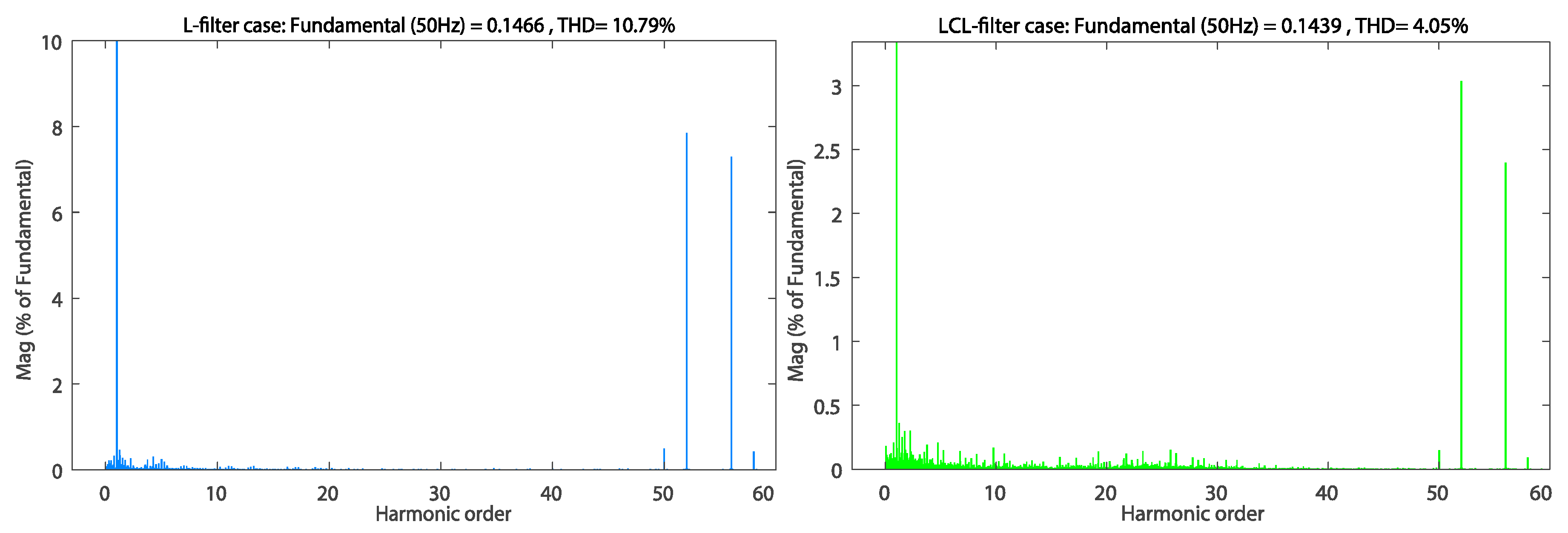
The quality of the three phase grid currents is investigated through measuring the THD of the AC grid currents. As depicted in Figure 12. It is obviously shown that the use of the LCL-filter achieves a better attenuation with a THD value about 4.05% for which the IEEE519-1992 standard limits are respected. Further analysis can be made to compare the THD of the AC grid currents in the case of using an L-filter based structure. According to the results of Figure 12, it is clear that the THD for adopting the LCL-filer is smaller than that using the L-filer type at the same value of inductance.

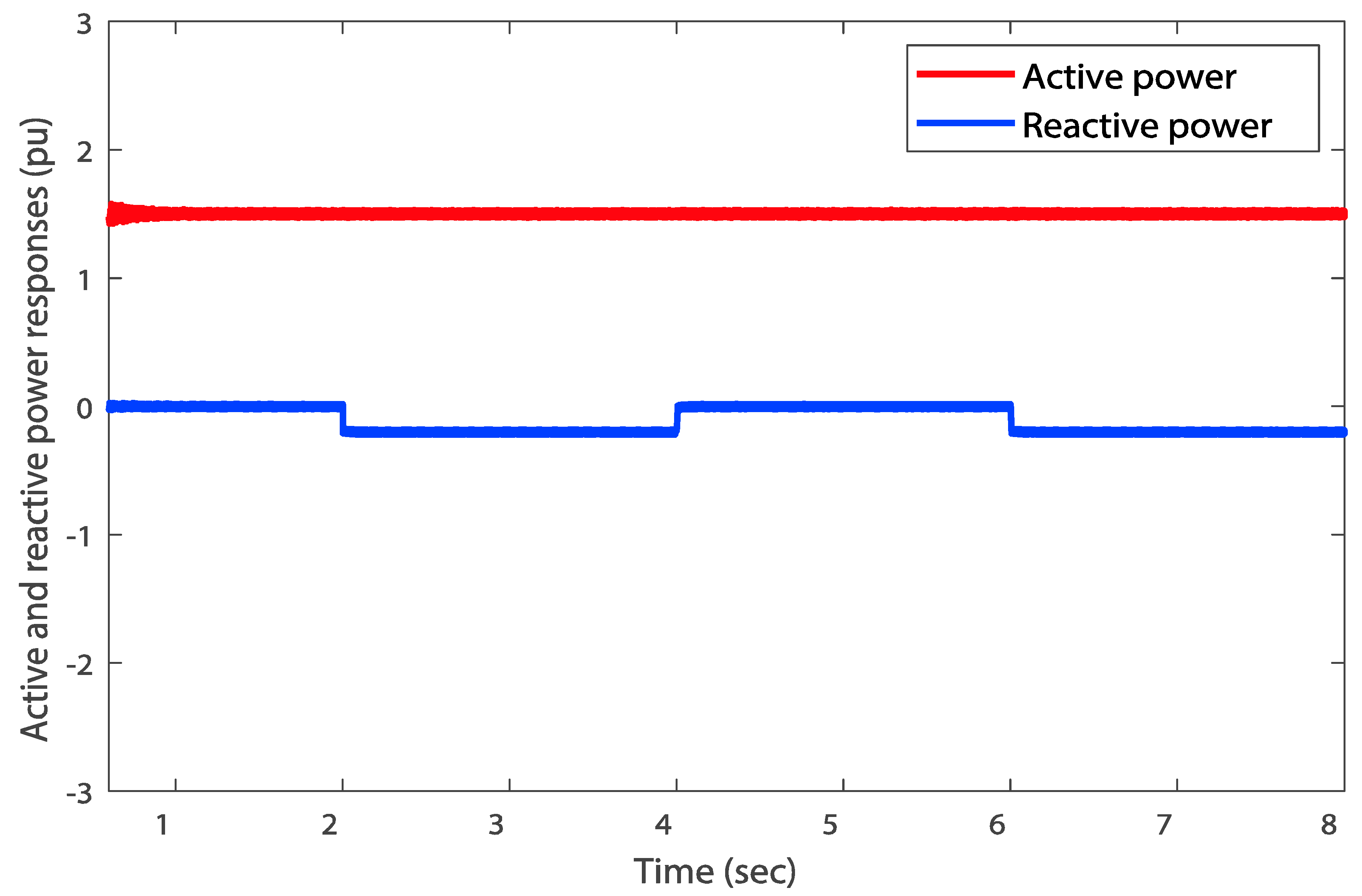
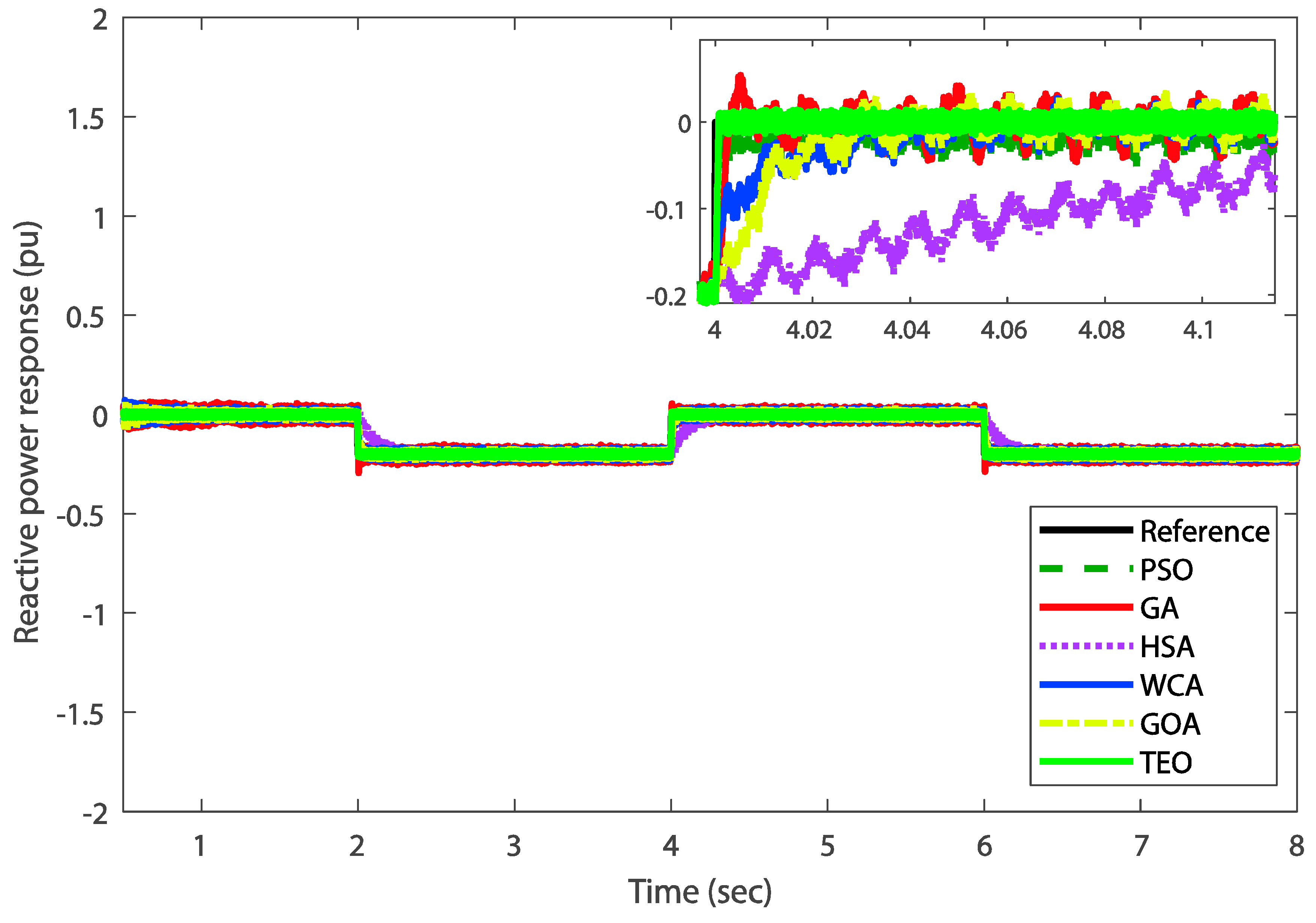
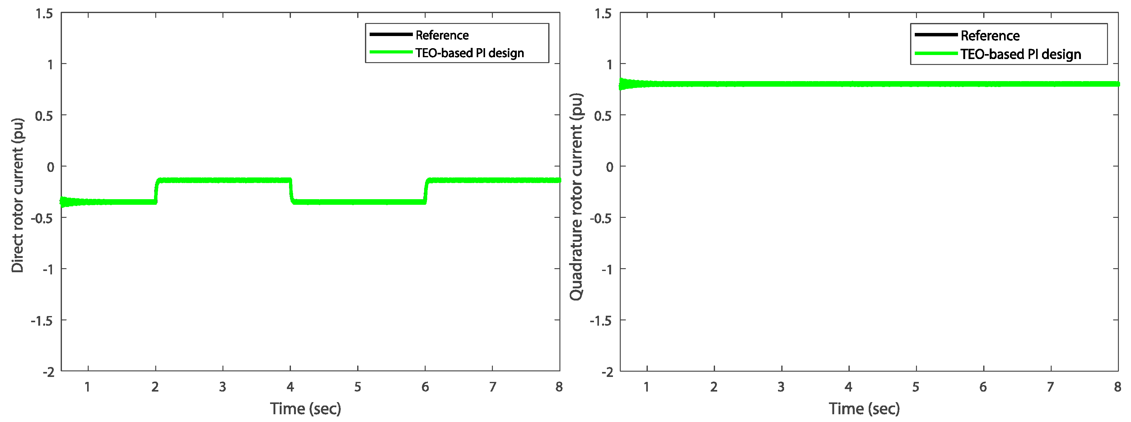
Referring to the RSC control results, the stator active and reactive powers can be regulated by controlling the q-axis rotor current. The reference value of stator active power is generated from a Maximum Power Point Tracking (MPPT) strategy to extract the maximum power from the wind. In addition, the value of reference reactive power is set at different step levels to check the performance of the proposed PI controllers. As shown in Figure 13, both active and reactive powers track effectively their reference values with good performance in terms of speed and damping dynamics. In addition, the decoupling between the active and reactive powers is perfectly assured and the DFIG extracts the maximum available power, which is approximately about 1.5 MW. Figure 14 demonstrates the control performance of the PI controller for the reactive power loop around its final set-point value based on different tuned PI methods. The aim is to show the difference between the optimization tuning-based methods. On the other hand, both left and right sides of Figure 15 show the tracking performance of the direct and quadrature rotor currents, respectively. Such tracking dynamics are perfectly performed and improved thanks to the proposed TEO-based tuning and control method.

6.2. Statistical Analysis and Comparison

In this part, the mean execution values related to the different optimization criteria are sorted to assess the best operating one according to its average objective function performance. Moreover, a statistical comparison based on the nonparametric Friedman and Bonferroni–Dunn is carried out by using these mean performances [30,31]. The average ranks for all the proposed methods based on the four performances indices are provided in

Table 6. Average Rank based statistical analysis of mean performances.

Algorithms	Indices								Average Rank
	IAE		ISE		ITSE		ITAE
	Score	Rank	Score	Rank	Score	Rank	Score	Rank
PSO	1.73	5	41.42	4	18.46	4	0.683	5	4.25
GA	1.67	4	37.25	3	17.96	1	0.650	1	2.25
HSA	1.60	3	35.51	2	23.18	6	0.683	4	3.75
WCA	1.59	2	45.88	6	18.32	3	0.659	3	3.75
GOA	2.01	6	44.06	5	19.83	5	0.688	6	5.5
TEO	1.58	1	33.46	1	18.24	2	0.658	2	1.5

. One can note that the proposed TEO metaheuristic has worthily attained the lowest average ranks compared to the remaining methods. A statistical analysis has been performed to highlight the importance of the TEO-based tuning method over other algorithms [32].

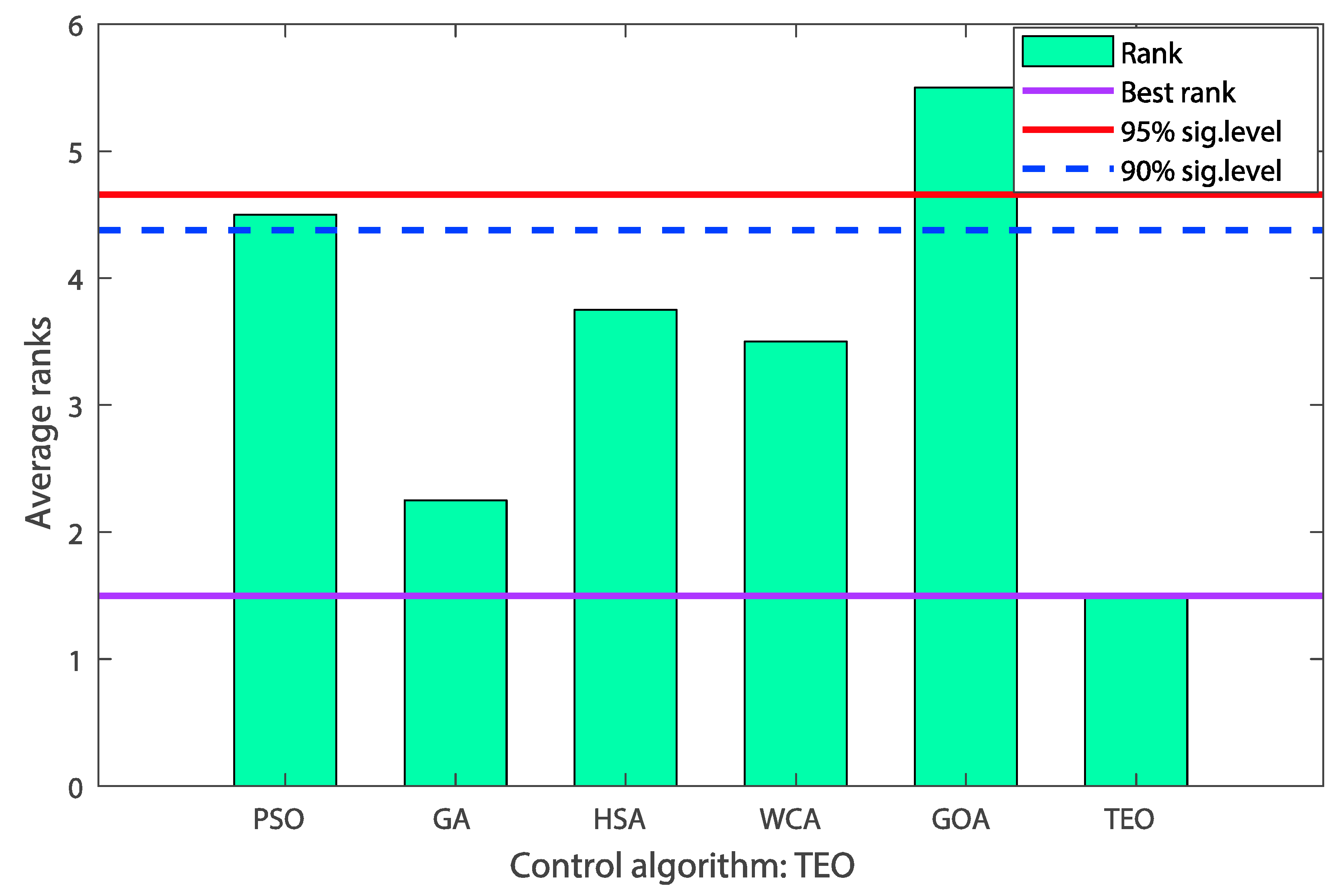
The Friedman test for six competitor algorithms ($m=6$) and four indices ($l=4$) provides the computed value ${\chi }_F^2=12.14$ of the $\chi$-distribution. The critical value of such a distribution with degrees of freedom $m-1=5$ and at confidence level $\alpha =0.05$ is equal to ${\chi }_{5,0.05}^2=11.07$. Since the above computed score is greater than this statistical value, the null hypothesis is declined. Moreover, for the Iman–Davenport test [30,31], the statistic is distributed with $m-1=5$ and $\left(m-1\right)\times \left(l-1\right)=15$ degrees of freedom. For this test, the null hypothesis is also rejected as the calculated value $F_F=4.64$ is greater than the critical value $F_{5,15,0.05}=2.9$ at the same significant level of confidence. All these statistical results indicate that there are significant differences among the performances of the reported algorithms for the optimization problem (19). Thus, the proposed TEO is found to be the most effective one having the best average Friedman ranking as given in Table 6. However, a Bonferroni–Dunn post-hoc test is called to investigate whether or not the proposed TEO algorithm is significantly better than another algorithm at the above considered level of confidence [32]. The corresponding Critical Differences (CD) of the reported algorithms at the confidence levels $\alpha =0.05$ (95% significance level) and $\alpha =0.1$ (90% significance level) are computed as ${\mathrm{CD}}_{0.05}=3.17$ and ${\mathrm{CD}}_{0.1}=2.88$, respectively. Figure 16 illustrates the graphical representation of the Bonferroni–Dunn test considering the TEO as the control algorithm [32,33].

The bar of the TEO algorithm is the lowest high among the reported algorithms and the heights of the bars corresponding to the PSO algorithm. The GOA method violates the horizontal lines of significant levels. This reveals that the TEO algorithm performs at least significantly better than these two algorithms over the solutions equality.

6.3. Computational Time Efficiency

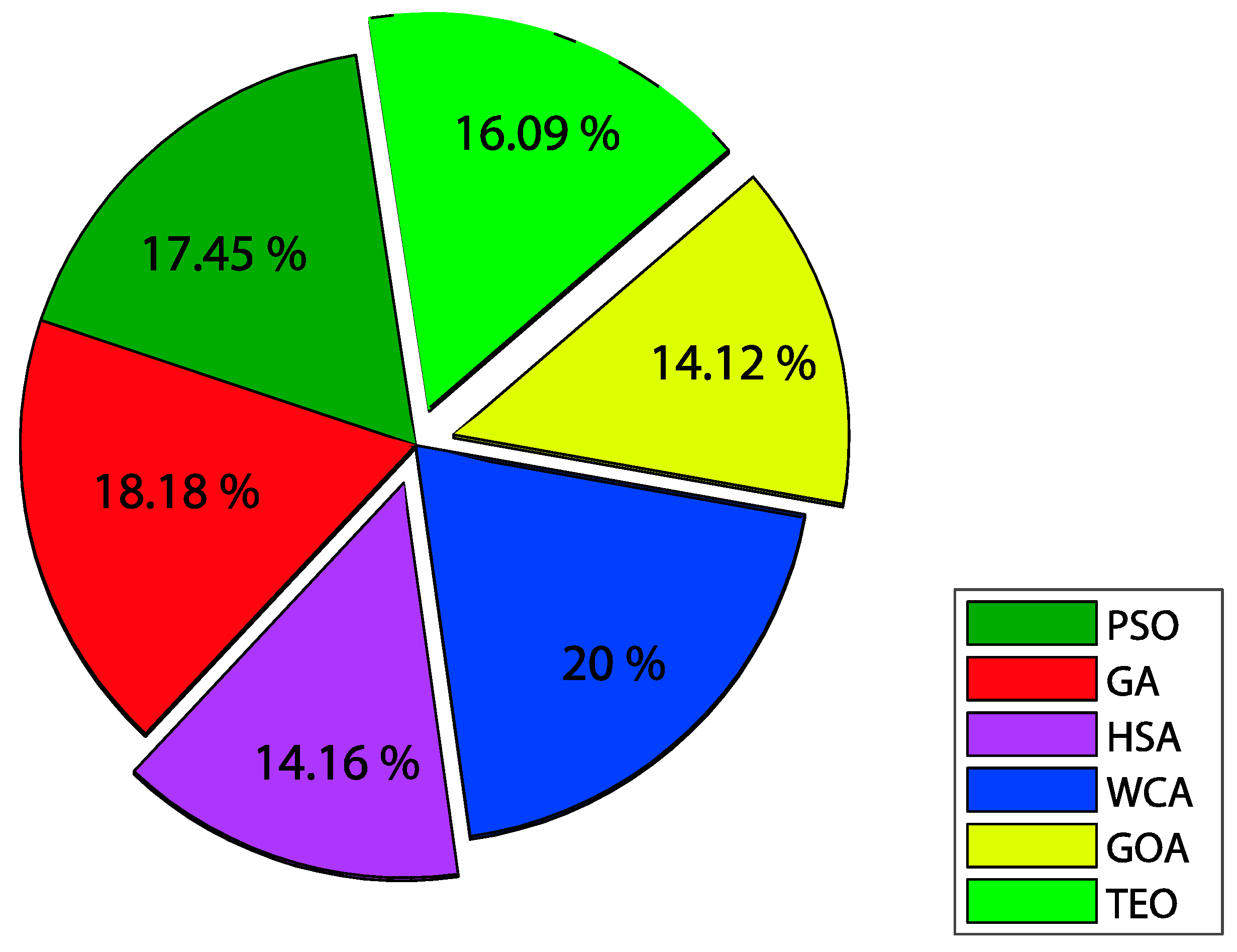
In this subsection, the average elapsed times of Table 3 are used to assess the computational efficiency of the reported algorithms. Such an algorithmic property of resource usage is quantified by the Computational Time Efficiency (CTE) metric defined as follows [34]:

$$CTE=\frac{E{T}_{algorithm}}{E{T}_{total}}(\%)$$

(28)

where $E{T}_{algorithm}$ and $E{T}_{total}$ denote the average and total elapsed times for the same index.

According to the ET measures of problem (19), the CTE for each algorithm over the reported optimization criterion is summarized in

Table 7. The computational time efficiency (CTE) of each algorithm over the four indices.

Index	Algorithms
	PSO	GA	HSA	WCA	GOA	TEO
IAE	18.01%	17.82%	15.81%	20.41%	12.66%	15.29%
ISE	19.52%	19.02%	13.24%	18.66%	13.32%	16.25%
ITSE	15.74%	19.19%	13.67%	20.11%	14.24%	17.07%
ITAE	16.20%	16.54%	13.63%	20.90%	16.83%	15.89%

.

In terms of computational efficiency, it can be observed from these results that the proposed TEO algorithm attained the second rank for IAE and ITAE criteria and the third and fourth ranks for ISE and ITSE criteria, respectively. Roughly, the HSA algorithm presents the best computational efficiency in terms of time resource usage. The GOA metaheuristic achieved the best average elapsed time as shown in Figure 17.

6.4. Sensitivity Analysis

In the TEO formalism, the parameters $c_1$ and $c_2$ are introduced to reduce the randomness of the algorithm over the course of iterations and to improve the exploration capabilities. The size of thermal memory TM is considered as a predefined parameter, which can enhance the performances of the algorithm without increasing the computational cost [3,24]. However, $pro$ is a user parameter that improves the global search capacity. For illustration purposes, the resolution of problem (19) is tested by changing these above main parameters. As shown in

Table 8. Comparison under different values of $c_1$ and $c_2$: IAE criterion.

Optimization Scenario	$\mathit{T}\mathit{M}=10,\mathit{p}\mathit{r}\mathit{o}=0.5\mathbf{and}{\mathit{N}}_{\mathit{i}\mathit{t}\mathit{e}\mathit{r}}=100$
	Worst	Mean	Best	STD
$c_1=0,c_2=0$	1.669	1.652	1.638	1.9 × 10−2
$c_1=1,c_2=0$	1.664	1.640	1.622	1.4 × 10−2
$c_1=0,c_2=1$	1.654	1.640	1.631	7.5 × 10−3
$c_1=1,c_2=1$	1.608	1.582	1.553	1.9 × 10−2

, the case with the parameters set $\left(c_1=1,c_2=1\right)$ shows the superiority of the optimization results compared to other scenarios. In addition, it can be seen from

Table 9. Comparison under different values of $TM$: IAE criterion.

Optimization Scenario	${\mathit{c}}_1=1,{\mathit{c}}_2=1,\mathit{p}\mathit{r}\mathit{o}=0.5\mathbf{and}{\mathit{N}}_{\mathit{i}\mathit{t}\mathit{e}\mathit{r}}=100$
	Worst	Mean	Best	STD
$TM=4$	1.699	1.694	1.689	3.5 × 10−3
$TM=8$	1.654	1.640	1.631	8.4 × 10−2
$TM=10$	1.608	1.582	1.553	1.9 × 10−2

that the user parameter $TM=10$ leads to obtain the best solutions. Finally,

Table 10. Comparison under different values of $pro$: IAE criterion.

Optimization Scenario	${\mathit{c}}_1=1,{\mathit{c}}_2=1,\mathit{T}\mathit{M}=10\mathbf{and}{\mathit{N}}_{\mathit{i}\mathit{t}\mathit{e}\mathit{r}}=100$
	Worst	Mean	Best	STD
$pro=0.20$	1.693	1.654	1.633	1.7 × 10−2
$pro=0.35$	1.678	1.617	1.575	5.2 × 10−2
$pro=0.50$	1.608	1.582	1.553	1.9 × 10−2

investigates the effect of the parameter $pro$ on the algorithm performance. The convergence of the TEO algorithm is always guaranteed under all these control parameters variations which shows the insensitivity of the proposed physics-inspired metaheuristic.

7. Conclusions

This paper proposes an intelligent metaheuristics-based design procedure to tune the outer-loop PI controllers for the direct power control scheme of DFIG-based energy conversion systems. In this study, only outer PI loops in the RSC and GSC circuits are optimized for the active and reactive powers and DC-link voltage dynamics. Since the reported classical techniques of PI controller tuning are tedious, time-consuming and not systematic, a TEO-based approach has been proposed and successfully implemented. The PI controllers tuning problem is firstly formulated as a constrained optimization program under nonlinear and non-smooth operational constraints. The introduced TEO algorithm is then employed separately to minimize several time-domain performance criteria such as IAE, ISE, ITAE and ITSE indices as objective functions. The proposed TEO-tuned PI controllers methodology improves the performance and robustness of the controlled DFIG-based energy converter in terms of rising time, settling time, and steady state indices. The classical trials-errors based methods of PI controllers tuning are no longer used and the design time is further reduced. To evaluate the performance superiority of the proposed TEO-based approach in finding the global minimum value of the objective function for various performance indices, a comparison study with the PSO, GA, HSA, GSO and WCA is performed. The demonstrative results exhibit that the proposed TEO gives very complete results in terms of global search capabilities, robustness and non-premature convergence. Finally, the statistical analysis is achieved by using the Friedman’s rank and Bonferroni-Dunn’s test. The corresponding results show that the proposed TEO-based method is a promising alternative approach for controlling the DFIG system by systematically tuning the unknown PI controllers’ parameters efficiently.

References

- Sahu, K.B. Wind Energy Developments and Policies in China: A Short Review. Renew. Sustain. Energy Rev. 2018, 81, 1393–1405. [Google Scholar] [CrossRef]
- Belmokhtar, K.; Doumbia, M.L.; Agbossou, K. Modelling and Fuzzy Logic Control of DFIG Based Wind Energy Conversion Systems. In Proceedings of the IEEE International Symposium on Industrial Electronics (ISIE), Hangzhou, China, 28–31 May 2012; pp. 1888–1893. [Google Scholar]
- Hu, J.; Nian, H.; Xu, H.; He, Y. Dynamic Modeling and Improved Control of DFIG under Distorted Grid Voltage Conditions. IEEE Trans. Energy Convers. 2011, 26, 163–175. [Google Scholar] [CrossRef]
- Liserre, M.; Blaabjerg, F.; Hansen, S. Design and Control of an LCL-Filter-based Three-Phase Active Rectifier. IEEE Trans. Ind. Appl. 2005, 50, 1281–1291. [Google Scholar] [CrossRef]
- Zhou, D.; Blaabjerg, F. Bandwidth Oriented Proportional-Integral Controller Design for Back-To-Back Power Converters in DFIG Wind Turbine System. IET Renew. Power Gen. 2017, 11, 941–951. [Google Scholar] [CrossRef]
- Hamane, B.; Doumbia, M.L.; Bouhamida, M.; Benghanem, M. Direct Active and Reactive Power Control of DFIG based WECS using PI and Sliding Mode Controllers. In Proceedings of the 40th Annual Conference of the IEEE Industrial Electronics Society, Dallas, TX, USA, 29 October–1 November 2014; pp. 2050–2055. [Google Scholar]
- Hamane, B.; Doumbia, M.L.; Bouhamida, M.; Draou, A.; Chaoui, H.; Benghanem, M. Comparative Study of PI, RST, Sliding Mode and Fuzzy Supervisory Controllers for DFIG based Wind Energy Conversion System. Int. J. Renew. Energy Res. 2015, 5, 1174–1185. [Google Scholar]
- Hamane, B.; Doumbia, M.L.; Bouhamida, M.; Draou, A.; Chaoui, H.; Benghanem, M. Modeling and Control of a Wind Energy Conversion System Based on DFIG Driven by a Matrix Converter. In Proceedings of the Eleventh International Conference on Ecological Vehicles and Renewable Energies, Monte Carlo, Monaco, 6–8 April 2016; pp. 1–8. [Google Scholar]
- Tanvir, A.A.; Merabet, A.; Beguenane, R. Real-Time Control of Active and Reactive Power for Doubly Fed Induction Generator (DFIG)-Based Wind Energy Conversion System. Energies 2015, 8, 10389–10408. [Google Scholar] [CrossRef] [Green Version]
- Bekakra, Y.; Attous, D.B. Optimal Tuning of PI Controller Using PSO Optimization for Indirect Power Control for DFIG Based Wind Turbine with MPPT. Int. J. Syst. Assur. Eng. Manag. 2014, 5, 219–229. [Google Scholar] [CrossRef]
- Vieira, J.P.A.; Nunes, M.N.A.; Bezerra, U.H. Design of Optimal PI Controllers for Doubly Fed Induction Generators in Wind Turbines Using Genetic Algorithm. In Proceedings of the IEEE Power and Energy Society General Meeting—Conversion and Delivery of Electrical Energy in the 21st Century, Pittsburgh, PA, USA, 20–24 July 2008; pp. 1–7. [Google Scholar]
- Asgharnia, A.; Shahnazi, R.; Jamali, A. Performance and Robustness of Optimal Fractional Fuzzy PID Controllers for Pitch Control of a Wind Turbine Using Chaotic Optimization Algorithms. ISA Trans. 2018, 79, 27–44. [Google Scholar] [CrossRef]
- Assareh, E.I.; Poultangari, I.; Tandis, E.; Nedaei, M. Optimizing the Wind Power Generation in Low Wind Speed Areas Using an Advanced Hybrid RBF Neural Network Coupled with the HGA-GSA Optimization Method. J. Mech. Sci. Technol. 2016, 30, 4735–4745. [Google Scholar] [CrossRef]
- Kaveh, A.; Dadras, A. A Novel Meta-Heuristic Optimization Algorithm: Thermal Exchange Optimization. Adv. Eng. Softw. 2017, 110, 69–84. [Google Scholar] [CrossRef]
- Gagra, S.K.; Mishra, S.; Sing, M. Performance Analysis of Grid Integrated Doubly Fed Induction Generator for a Small Hydropower Plant. Int. J. Renew. Energy Res. 2018, 8, 2310–2323. [Google Scholar]
- Qiao, W. Dynamic Modeling and Control of Doubly Fed Induction Generators Driven by Wind Turbines. In Proceedings of the IEEE/PES Power Systems Conference and Exposition, Seattle, DC, USA, 15–18 March 2009; pp. 1–8. [Google Scholar]
- Xu, D.; Blaabjerg, F.; Chen, W.; Zhu, N. Advanced Control of Doubly Fed Induction Generator for Wind Power Systems, 1st ed.; John Wiley & Sons: New York, NY, USA, 2018. [Google Scholar]
- Hato, M.M.; Bouallègue, S.; Ayadi, M. Water cycle algorithm-tuned PI control of a doubly fed induction generator for wind energy conversion. In Proceedings of the 9th International Renewable Energy Congress (IREC), Hammamet, Tunisia, 20–22 March 2018; pp. 1–6. [Google Scholar]
- Åström, A.K.; Hägglund, T. Advanced PID Control; ISA-Instrumentation, Systems and Automation Society: Research Triangle Park, NC, USA, 2006. [Google Scholar]
- Bouallègue, S.; Haggège, J.; Ayadi, M.; Benrejeb, M. PID-Type Fuzzy Logic Controller Tuning based on Particle Swarm Optimization. Eng. Appl. Artif. Intel. 2012, 25, 484–493. [Google Scholar] [CrossRef]
- Qu, B.Y.; Zhu, Y.S.; Jiao, Y.S.; Wu, M.Y.; Suganthan, P.N.; Liang, J.J. A Survey on Multi-objective Evolutionary Algorithms for the Solution of the Environmental/Economic Dispatch Problems. Swarm Evol. Comput. 2018, 8, 1–11. [Google Scholar] [CrossRef]
- Gong, L.; Cao, W.; Liu, K.; Zhao, J.; Li, X. Spatial and Temporal Optimization Strategy for Plug-in Electric Vehicle Charging to Mitigate Impacts on Distribution Network. Energies 2018, 11, 1373. [Google Scholar] [CrossRef]
- Zhang, X.; Yang, J.; Wang, W.; Jing, T.; Zhang, M. Optimal Operation Analysis of The Distribution Network Comprising a Micro Energy Grid based on an Improved Grey Wolf Optimization Algorithm. Appl. Sci. 2018, 8, 923. [Google Scholar] [CrossRef]
- Kaveh, A.; Ghazaan, M.I. Enhanced Colliding Bodies Optimization for Design Problems with Continuous and Discrete Variables. Adv. Eng. Softw. 2014, 77, 66–75. [Google Scholar] [CrossRef]
- Geem, Z.W.; Kim, J.H.; Loganathan, G.V. A New Heuristic Optimization Algorithm: Harmony Search. Sage J. 2012, 76, 60–68. [Google Scholar]
- Saremi, S.; Mirjalili, S.; Lewis, A. Grasshopper Optimization Algorithm: Theory and Application. Adv. Eng. Softw. 2017, 105, 30–47. [Google Scholar] [CrossRef]
- Blasko, V.; Kaura, V. A Novel Control to Actively Damp Resonance in Input LC Filter of a Three-Phase Voltage Source Converter. IEEE Trans. Ind. Appl. 1997, 33, 542–550. [Google Scholar] [CrossRef]
- Bingi, K.; Ibrahim, R.; Karsiti, M.N.; Chung, T.D.; Hassan, S.M. Optimal PID control of pH neutralization plant. In Proceedings of the 2nd IEEE International Symposium on Robotics and Manufacturing Automation, Ipoh, Malaysia, 25–27 September 2016; pp. 1–6. [Google Scholar]
- Mishra, K.P.; Kumar, V.; Rana, K.P.S. Stiction combating intelligent controller tuning a comparative study. In Proceedings of the International Conference on Advances in Computer Engineering and Application, Ghaziabad, India, 19–20 March 2015; pp. 534–541. [Google Scholar]
- Raghuwanshi, B.S.; Shukla, S. Generalized Class-Specific Kernelized Extreme Learning Machine for Multiclass Imbalanced Learning. Expert. Syst. 2019, 121, 244–255. [Google Scholar] [CrossRef]
- Zeng, F.; Zhang, W.; Zhang, S.; Zheng, N. Re-Kissme: A Robust Resampling Scheme for Distance Metric Learning in the Presence of Label Noise. Neurocomputing 2019, 330, 138–150. [Google Scholar] [CrossRef]
- Sadhu, A.K.; Konar, A.; Bhattacharjee, A.T.; Das, S. Synergism of Firefly Algorithm and Q-Learning for Robot Arm Path Planning. Swarm Evol. Comput. 2018, 43, 50–68. [Google Scholar] [CrossRef]
- Liu, Y.; Chen, S.; Guan, B.; Xu, P. Layout Optimization of Large-Scale Oil–Gas Gathering System based on Combined Optimization Strategy. Neurocomputing 2019, 332, 159–183. [Google Scholar] [CrossRef]
- Sababha, M.; Zohdy, M.; Kafafy, M. The Enhanced Firefly Algorithm Based on Modified Exploitation and Exploration Mechanism. Electronics 2018, 7, 132. [Google Scholar] [CrossRef]
Figure 1.
Configuration of the Doubly Fed Induction Generator (DFIG)-based Wind Energy Converter System (WECS).
Figure 2.
Proportional-Integral (PI) control scheme for the inner current loop of the RSC.
Figure 3.
Design of the PI controller current loop of grid side converter.
Figure 4.
The proposed control algorithm applied to the DFIG system.
Figure 5.
Pairs of environment and cooling objects.
Figure 6.
Flowchart of the proposed Thermal Exchange Optimization (TEO)-tuned PI controllers’ parameters.
Figure 7.
Convergence rates comparison: (a) IAE criterion; (b) ISE criterion; (c) ITAE criterion; (d) ITSE criterion.
Figure 8.
Box-and-Whisker plot of optimization problem (19): (a) IAE criterion; (b) ISE criterion; (c) ITAE criterion; (d) ITSE criterion.
Figure 9.
DC-link voltage responses against step changes for different-tuned PI controllers.
Figure 10.
Quadrature grid current responses against a step change for different-tuned PI controllers.
Figure 11.
Bode plot of the open loop grid current loop: with and without passive damping based technical optimum tuning.
Figure 12.
Harmonics spectrum of the AC grid currents.
Figure 13.
Time-domain variations of the TEO-tuned PI controlled active and reactive powers.
Figure 14.
Performance comparison of the controlled reactive power under different PI controllers’ tuning methods.
Figure 15.
Time-domain variations of the TEO-based control of the direct and quadrature rotor currents.
Figure 16.
Graphical representation of Bonferroni–Dunn’s test for problem (19).
Figure 17.
Average elapsed time over all criteria for the introduced algorithms.