The Archimedes’ Constant, π Seen by Mechanical Engineers

Abstract

Probabilistic engineering mechanics is used to relate the value of $\pi$ with one of the main parameters in fracture mechanics. It proposes an engineering method to obtain the value of it from engineering data without involving any geometrical Euclidian’s circle’s data measurement or analysis. It is the first trial in studying the use of fracture mechanics to determine the value of ratio of circumference and diameter of Euclidean’s circles indirectly, and subsequently evaluate the number of the digits actually needed in fracture mechanics and engineering purposes.

1. Introduction

Probabilistic engineering mechanics is used in this exploratory article partly to commemorate the death of a Nobel Laurette on 1 February 2012, may she rest in peace. Born 2 July 1923 in Prowent, Poland, the Nobel Laurette, Wislawa Szymborska, had always fascinated with $\pi$ and, therefore, she wrote a poem on it [1]. The beginning of the poem is:

$$\begin{array}{c}\mathit{\pi }\\ The admirable number \pi : three point one four one. All the following\\ digits are also just a start, five nine two because it never ends. It can’t\\ be grasped, six five three five, at a glance, eight nine, by calculation,\\ seven nine, through imagination, or even three two three eight in jest,\\ or by comparison four six to anything two six four three in the world.\\ \dots \dots \left(continued\right)\dots \dots \end{array}$$

Although it is commonly known as 3.14, the value of ‘$\pi$’is $irrational$ and can never be expressed exactly as a fraction of integers in both the numerator and denominator. It also can never be expressed as a finite sequence of algebraic operations on integers. It is a non-constructible, as it is impossible to square the circle as was proved by lots of great mathematicians, such as Lindemann back in 1882 [2]. Throughout history, there has been much effort to determine its value more accurately. The fascination with it is carried over into cultures other than mathematics. Possibly because of the simplicity of its definition, it became more entrenched in popular culture than almost any other mathematical concepts [3] since 1650 B.C, as it is recorded in the Egyptian rhind papyrus that shows $\pi \approx 4\times {\left(\frac{8}{9}\right)}^2$ [4]. It is also a common ground among researchers in other fields as well. It is truly the world’s most mysterious number [5]. Reports on the latest calculations of it are common news items, and some report the accuracy up to over several trillion decimal digits, and as you read this article it is probably even more because the computer is still calculating it [6].

There is no doubt that a lot of formulae used in mathematics, economics, science, and engineering use $\pi$. This emphasizes the importance and significance of the mathematical constant, $\pi$ [7,8]. Researchers from almost any kind of field are fascinated to know the exact value of it. This short technical note discusses its basic concept briefly, historical chronology and scientific quest of research on it, followed by our original concept of the non-geometrical approach on the approximation of the $\pi$. Using the reverse engineering concept, we formulate the number of the digits of $\pi$ needed for engineering computation.

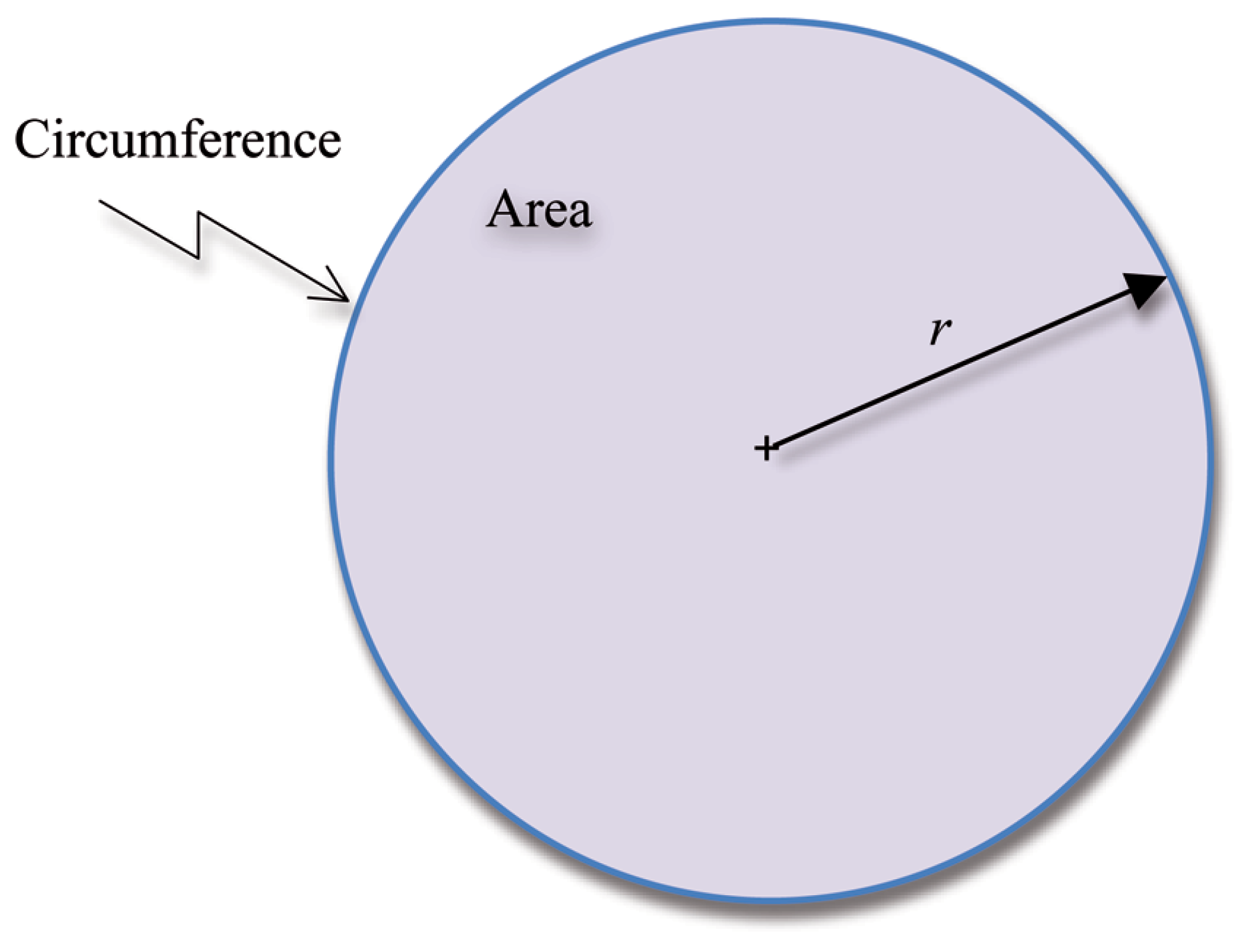
2. Basic Concept

The letter $\pi$ is the first letter in a Greek word of ‘$\pi \epsilon \rho \iota \phi \acute{\epsilon }\rho \epsilon \iota \alpha$’, periphery, or ‘$\pi \epsilon \rho \iota \mu \epsilon \tau \rho o\varsigma$’, perimeter, or circumference. Figure 1 shows the basic concept of the traditional computation of constant $\pi$. It is defined as:

$$\pi =\frac{C}{2r}$$

(1)

or

$$\pi =\frac{A}{r^2},$$

(2)

where C is the circumference, A is the area, and r is the radius of a Euclidean’s circle. Although the definition is so simple, the value of $\pi$ can never be calculated analytically. The truncation of decimal of $\pi$ to 11 is known to be good enough to estimate the circumference of any circle that fits inside the earth with an error of less than one millimeter, and the truncation to 39 decimals is known to be sufficient to estimate the circumference of any circle that fits in the observable universe with precision comparable to the radius of a hydrogen atom [9]. Therefore, from the engineering point of view, finding the exact value of $\pi$ seems to be out of necessity. However, engineers are human too. Their satisfactions and fascinations are not necessarily expressible in words or in equations, although only a few engineers are capable of expressing their feeling on their fascinations like the Nobel Laurette in literacy, whose poem is quoted in the introduction part.

3. Compilation of the Values of $\mathbf{\pi }$

Table 1. Main equations pertaining to the value estimation of $\pi$.

Value	Inventor and Remarks	Source
$\pi \approx 4\times {\left(\frac{8}{9}\right)}^2$	Value used by ancient Egyptians (1650 B.C.)	[4]
$\frac{223}{71}<\pi <\frac{22}{7}$	Archimedes (287–212 B.C.)	[10]
$3.141024<\pi <3.1415927$	Zu (429–500 A.D.)	[10]
$\pi \approx 2\times \frac{2}{\sqrt{2}}\times \frac{2}{\sqrt{2+\sqrt{2}}}\dots .$	Viette (1593)	[3]
$\pi \approx 4{\sum }_{k=0}^{\infty }(\frac{{(-1)}^k}{2k+1})$	Madhava–Leibniz series. Slow to converge	[11]
$\pi \approx \sqrt{12}{\sum }_{k=0}^{\infty }(\frac{{(-3)}^k}{2k+1})$	Modified Madhava–Leibniz series. Better convergence, capable of producing accurate 11 digits	[16]
$\frac{\pi }{2}\approx {\prod }_{k=1}^{\infty }\frac{{\left(2k\right)}^2}{{\left(2k\right)}^2-1}$	Walli’s product (1650)	[12]
$\pi \approx 3{\sum }_{n=0}^{\infty }\frac{\left(\genfrac{}{}{0pt}{}{2n}{n}\right)}{{16}^n(2n+1)}$	Isaac Newton	[13]
$\frac{1}{\pi }\approx \frac{2\sqrt{2}}{9801}{\sum }_{k=0}^{\infty }(\frac{\left(4k\right)!(1103+26390k}{{(k!)}^4{396}^{4k}})$	Srinivasa Ramanujan	[14]
$\pi \approx {\sum }_{k=0}^{\infty }\frac{1}{{16}^k}(\frac{4}{8k+1}-\frac{2}{8k+4}-\frac{1}{8k+5}-\frac{1}{8k+6})$	Bailey et al.	[15]

shows major findings of the empirical $\pi$, although in reality many more than those are available; here, the compilation from representative sources is tabulated in the chronological order [4,10,11,12,13,14,15]. It is worth noting that those empirical values are not necessarily derived based on the geometry anymore, instead they can be derived from other disciplines. Several studies deriving the value of $\pi$ without a geometrical approach are also available, e.g., economics [10]. For our purpose, the value of $\pi$ used for error estimation is based on:

$$\pi =3.141592653589,$$

(3)

which is 13 significant numbers. This value was a computed value based on the formula developed by Viete [3].

4. Obtaining $\mathbf{\pi }$ from Engineering Data

The concepts of fracture mechanics are concerned with the basic ideas for developing methods to predict the load-carrying capabilities of structures containing cracks, although in here the concept is used solely for the purpose of deriving the value of ‘empirical-$\pi$’ from fracture mechanics point of view. The approach is based on a mathematical description of the characteristic stress field surrounding a crack in a loaded body, see Figure 2. To explore the characteristics of the stress field surrounding a crack in a loaded body, one can start from the Westergaard function [16]. The Westergaard function is a complex solution to the Airy stress functions. To do this, consider a coordinate system $x,y,z$ in a stressed solid. At each point $(x,y,z)$, one can define the stresses ${\sigma }_x,{\sigma }_y,{\sigma }_z,{\tau }_{xy},{\tau }_{xz},{\tau }_{yz}$. Neglecting the body forces, for two-dimensional problems, the equilibrium equations are

$$\frac{\partial {\sigma }_x}{\partial x}+\frac{\partial {\tau }_{xy}}{\partial y}\mathrm{and}\frac{\partial {\sigma }_y}{\partial y}+\frac{\partial {\tau }_{xy}}{\partial x}.$$

(4)

In addition, recall their relations with the elastic strain:

$${ϵ}_x=\frac{\partial u}{\partial x}{ϵ}_y=\frac{\partial v}{\partial y}{\gamma }_{xy}=\frac{\partial u}{\partial y}+\frac{\partial v}{\partial x}.$$

(5)

The equilibrium equation in (4) is automatically satisfied if

$${\sigma }_x=\frac{{\partial }^2\psi }{\partial y^2}{\sigma }_y=\frac{{\partial }^2\psi }{\partial x^2}{\tau }_{xy}=\frac{{\partial }^2\psi }{\partial x\partial y}$$

(6)

with the stress–strain relation

$$E{ϵ}_x={\sigma }_x-\nu {\sigma }_{y}E{ϵ}_y={\sigma }_x-\nu {\sigma }_x\frac{E{\gamma }_x}{2(1+\nu )}={\tau }_{xy}.$$

(7)

The function $\psi$ is called the Airy stress function. Substitution of Equations (5) and (6) into Equation (7) and differentiating twice leads to the following compatibility:

$${▿}^2\left({▿}^2\psi \right)=0.$$

(8)

One can then define a complex function

$$\psi =\mathrm{Re}\overline{\overline{Z}}+y\mathrm{Im}\overline{Z},$$

(9)

where $\frac{d\overline{\overline{Z}}}{dz}=\overline{Z}$, $\frac{d\overline{Z}}{dz}=Z$, and $\frac{dZ}{dz}=Z^{\prime }$. The position at which the equation valid is in front of the crack. With the Cauchy–Riemann equation, it follows that

$${▿}^2\mathrm{Re}\overline{\overline{Z}}={▿}^2\mathrm{Im}Z=0.$$

(10)

Therefore, the stress becomes:

$${\sigma }_x=\mathrm{Re}Z-y\mathrm{Im}{Z}^{\prime }{\sigma }_y=\mathrm{Re}Z+y\mathrm{Im}{Z}^{\prime }.{\tau }_{xy}=-y\mathrm{Re}{Z}^{\prime }$$

(11)

The function is analytic except for $(-a\le x\le a,y=0)$. The boundary stresses follow $\mid z\mid \to \infty$, the results are ${\sigma }_x={\sigma }_y=\sigma$ and ${\tau }_{xy}=0$, and on the crack surface $\sigma ={\tau }_{xy}=0$, which means that the boundary conditions are satisfied. It is more convenient to convert to a coordinate system with the origin at the crack tip, hence z should be replaced by $(z+a)$. Turning to the general problem, which is shown in Figure 3 that has the form:

$$Z=\frac{f\left(z\right)}{\sqrt{z}}.$$

(12)

The required real and constant value of $f\left(z\right)$ at the crack tip is given by the notation $K_I$, hence

$$Z=\frac{K_I}{\sqrt{2\pi z}}.$$

(13)

With some mathematical manipulation [16], the stress singularity in front of a crack tip can then be expressed by

$${\sigma }_{ij}=\frac{K_I}{\sqrt{2\pi r}}{f}_{ij}\left(\theta \right)$$

(14)

or

$$\pi =\frac{K_I^2}{2r{\sigma }_{ij}^2}{f}_{ij}^2\left(\theta \right),$$

(15)

where r and $\theta$ are the polar coordinates of a point with respect to the crack tip, and $K_I$ is the stress intensity factor, see Figure 3. Taking the polar coordinate from the origin, Equation (15) can then be simplified for our purpose to only an element in the vertical direction:

$$\pi =\frac{K_I^2}{2r{\sigma }_{yy}}co{s}^2\frac{\theta }{2}{\left(1+si{n}^2\frac{\theta }{2}si{n}^2\frac{3\theta }{2}\right)}^2.$$

(16)

Here, Equation (16) is our tool to evaluate the value of the $\pi$. The convergence of the value can then be used to evaluate to determine how many decimals needed from the engineering mechanics point of view.

5. Computational and Experimental Approaches

The computational approach is legitimate to be used here because K and ${\sigma }_{yy}$ are independently calculated without the need to use geometrical information pertaining to Eucledian’s circle. To make engineering sounds of the analysis, a computational model that is close to a real engineering experiment is constructed in addition to an experiment. The model here is homogeneous material having the shape of a CT (compact tension) specimen according to ASTM E647 and E08 [17,18] standards. The following steps were taken:

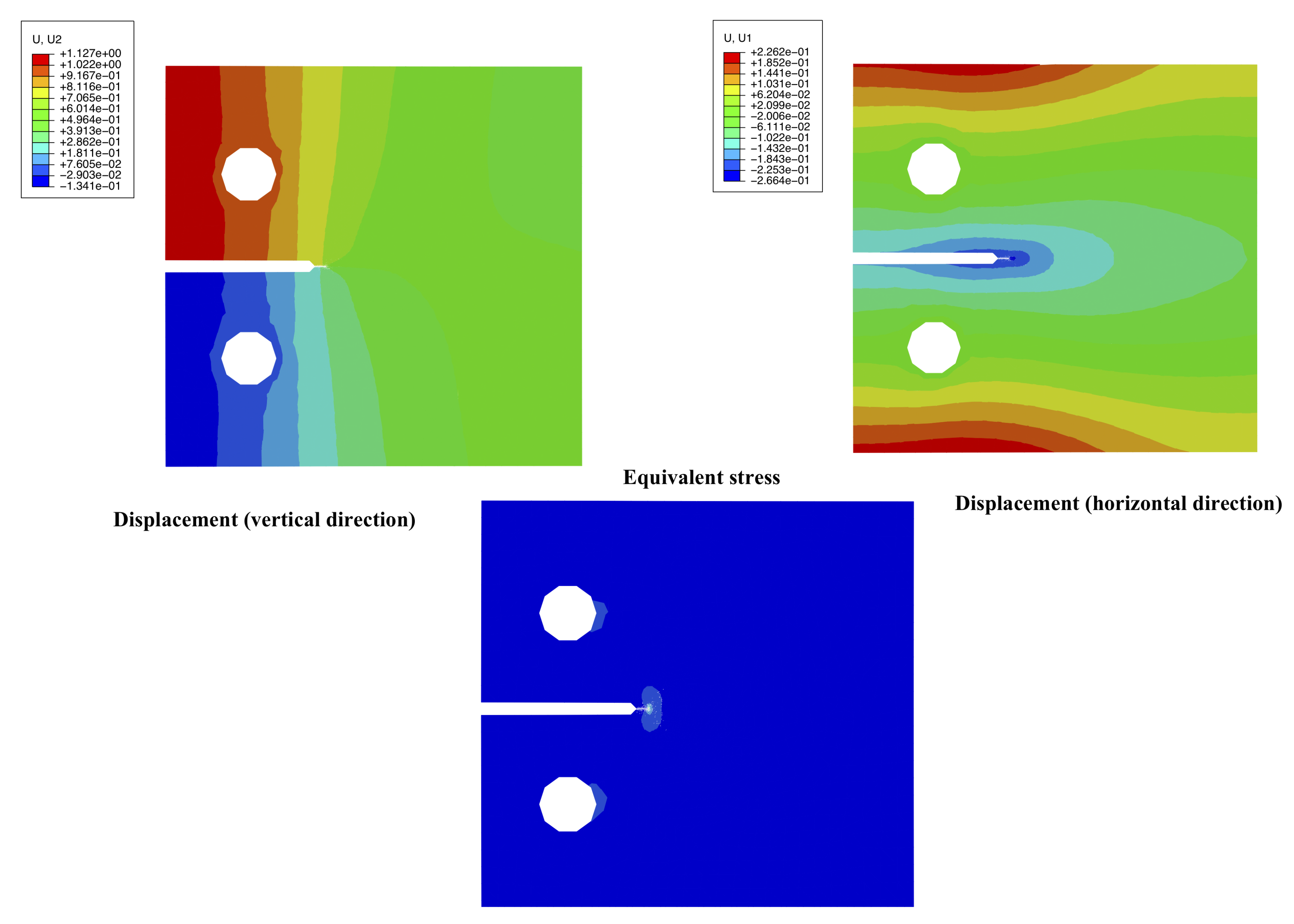
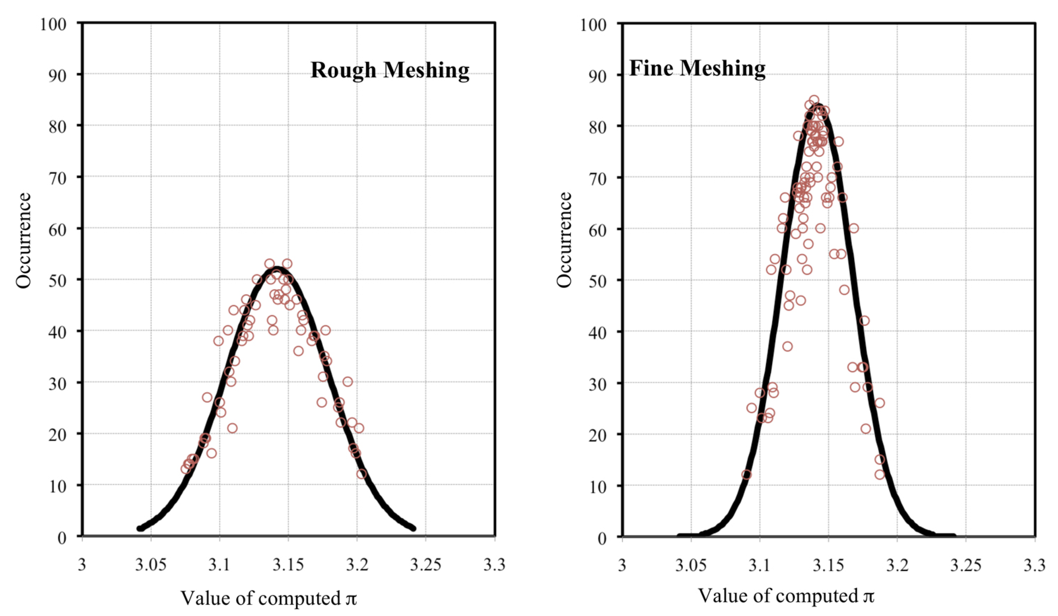
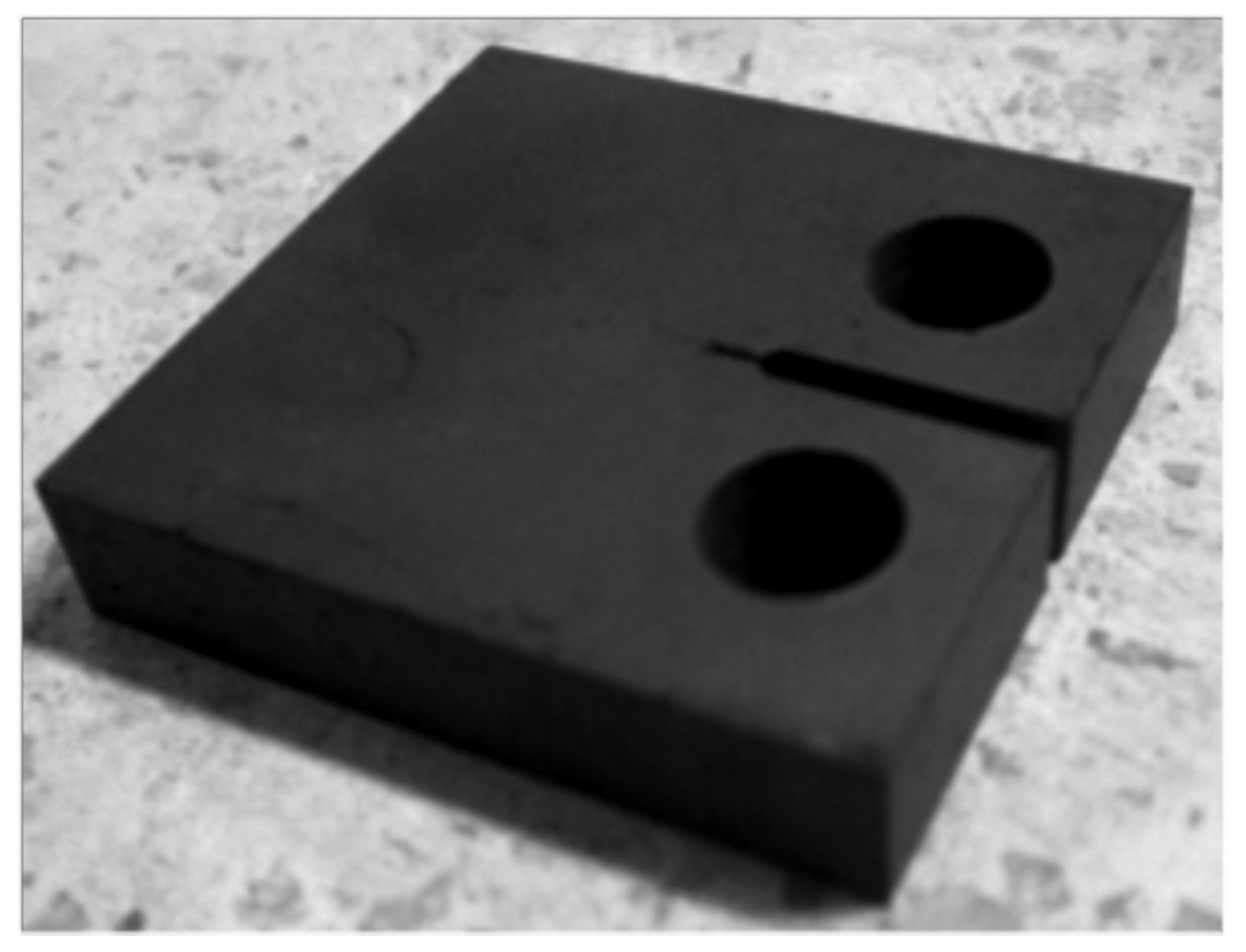
• Model creation, load and boundary condition applications. For this purpose, two different meshing sizes were employed, namely rough (approximately 2000 nodes) and fine (approximately 6000 nodes).
  →Figure 4.
• Obtain the nodal/element information of $\theta$ and r to compute each individual value of $\frac{K_I^2}{2r}co{s}^2\frac{\theta }{2}{\left(1+si{n}^2\frac{\theta }{2}si{n}^2\frac{3\theta }{2}\right)}^2$.
• Obtain the nodal/element values of ${\sigma }_{yy}$.
• Compute the value of $\pi$ according to Equation (16) for each individual node/element.
• Generate the graph to evaluate the convergence value of $\pi$ using Equation (16).
  →Figure 5.
• Go back to step 1, mesh the model with different mesh size, and follow the same procedure.

The results are basically two different Gaussian like curves (Figure 5). Based on these curves, the FWHM ( full width at half maximum) can then be estimated. In our case here, the rough meshing, the FWHM is approximated by the following the lines shown in the figure:

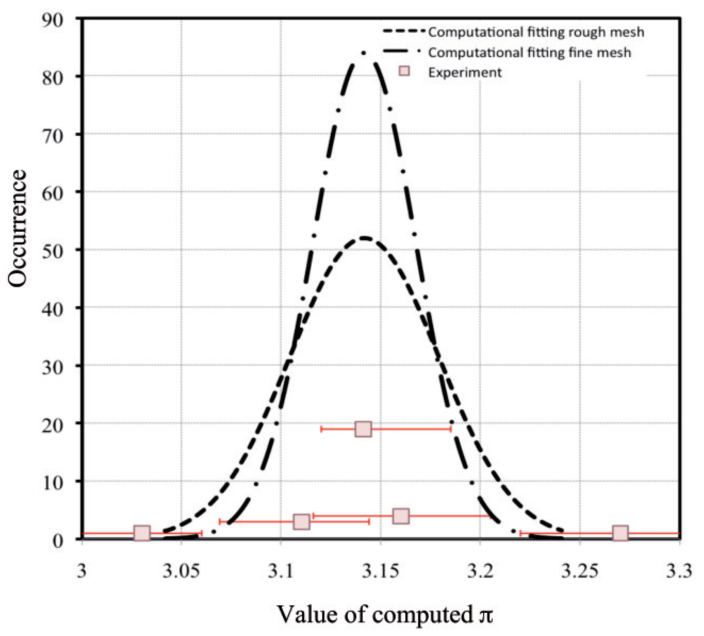
• Generalized estimation:

  $$f\left(x\right)=\frac{1}{\sigma \sqrt{2\pi }}·\mathrm{Exp}\left[-\frac{{(x-x_0)}^2}{2{\sigma }^2}\right],$$

  $$f\left(x\right)=C_1·\mathrm{Exp}\left[-\frac{{(x-x_0)}^2}{C_2·{\sigma }^2}\right],$$
• Curve fitting for data obtained from rough meshing (based on $\approx 2000$ data points):

  $$f\left(x\right)=52·\mathrm{Exp}\left[-\frac{{(x-\pi )}^2}{3.1\times {0.03}^2}\right],$$

  $$⇝\mathrm{FWHM}\approx 0.086.\mathrm{Therefore},\mathrm{our}\left(\mathrm{engineering}\pi \right)\approx \left(\mathrm{true}\pi \right)\pm 0.043$$

  $$⇝:3.098\le \pi \le 3.184,$$
• Curve fitting for data obtained from fine meshing (based on $\approx 6000$ data points):

  $$f\left(x\right)=83·\mathrm{Exp}\left[-\frac{{(x-\pi )}^2}{1.5\times {0.03}^2}\right],$$

  $$⇝\mathrm{FWHM}\approx 0.050.\mathrm{Therefore},\mathrm{our}\left(\mathrm{engineering}\pi \right)\approx \left(\mathrm{true}\pi \right)\pm 0.025$$

  $$⇝:3.116\le \pi \le 3.166.$$

Even though the FWHM here is based on the interpolation of the computational results, the experimental data within the framework of fracture mechanics also showed similarly due to the modeling that mimics the experiment. Therefore, the data obtained and used in the computational approach here simulated an ideal engineering experiment. Experimental data were not taken solely for this purpose; instead, it was for another purpose [16,19]. However, the data were then processed to relate $\pi$ and $K_I^2$ as it is described in Equation (16). The samples used were compact tension specimens. While the detailed data collection method is beyond the topic of this paper, and the readers are to consult to the reference directly [19], for the sake of the reader’s convenience, the method is briefly highlighted here. Figure 6 is the representative specimen used in the experiment. The stress intensity factor K for standard CT specimen geometry was calculated as follows: [17,18]:

$$K=\frac{P}{B\sqrt{W}}\frac{2+\alpha }{{(1-\alpha )}^{3/2}}\left(0.886+4.64\alpha -13.32{\alpha }^2+14.72{\alpha }^3-5.6{\alpha }^4\right),$$

(17)

where B and W are the specimen’s thickness and width, respectively. $\alpha$ is the relative crack length ($a/W$), and P is the applied load. The value of stress ${\sigma }_{yy}$ was obtained by the surface strain measurements outside the plastic zone area. The plastic zone sizes and definition are the ones defined and calculated in the references published previously [16], with the assumption of the plane stress governing rule. Figure 7 shows the distribution of the values of the $\pi$ calculated from experimental results. In the figure, the curve fittings of the same distribution by computational approaches were also plotted.

6. Discussion

The research shows that $\pi$ can be obtained empirically using a fracture mechanics concept too. This fact is not surprising as it can also be obtained by other data, including economics, and even societal human behaviors [7,8]. Our method is in a way similar to that of Buffon’s Needle [20]. It is one of the classic problems in the field of geometrical probability for finding $\pi$ by the experiment. It involves dropping a needle on a lined sheet of paper and determining the probability of the needle crossing one of the lines on the page. The problem also can be solved using integral geometry. The remarkable result is that the probability is directly related to the value of $\pi$ and can be used to design a Monte Carlo method for approximating the number of $\pi$.

Our observations of the answers clarify that, based on the rough meshing, $3.098\le \pi \le 3.184$, while, based on the fine meshing, $3.116\le \pi \le 3.166$. The difference of the result of rough meshing and fine meshing is only on the standard deviation. The fine meshing gives the smaller standard deviation, while the mean of both distributions remains the same. Thus, as the sample size increases, the standard deviation of the means decreases. This implies that actually engineering data only needs no more than three significant numbers of $\pi$. Experimental data show that an even lower digit number is actually needed. The fine meshing data shows that it requires three significant numbers, while the rough one requires only two significant numbers. This once again reiterated the fact that the truncation of decimal of $\pi$ to 11 is good enough to estimate the circumference of any circle that fits inside the earth with an error of less than one millimeter, while modern engineering relies on extensive empirical equations based on experimental data that inherit large errors. The fact that many researchers and enthusiasts produce billions or even trillions of significant numbers is clearly beyond the engineering needs.

7. Conclusions

An engineering approach that does not directly involve any circle/geometrical analysis related to a circle was used to derive $\pi$ here. Using the old school engineering rule of thumb, it has been agreed that conventional engineering fracture mechanics require no more than three digits of $\pi$, although nowadays computer usage automatically generates the number of digits depending on the type of the computer used as well as on the software used.

References

- Nobelprize.org. Wislawa Szymborska—A Biography. Available online: http://www.nobelprize.org/nobelprizes/literature/laureates/1996/szymborska-bio.html (accessed on 22 July 2019).
- Lindenmann, F. Uber die zahl π. Math. Ann. 1982, 20, 213–215. [Google Scholar]
- Berggren, L.; Borwein, J.; Borwein, P. Pi: A Source Book; Springer: New York, NY, USA, 2004. [Google Scholar]
- Gillings, R. Mathematics in the Time of the Pharaohs; Dover: Mineola, NY, USA, 1982. [Google Scholar]
- Posamentier, A.S.; Lehmann, I. A Biography of the World’s Most Mysterious Number; Prometheus Books: Amherst, NY, USA, 2004. [Google Scholar]
- Takahashi, D. Parallel implementation of multiple-precision arithmetic and 2,576,980,370,000 decimal digits of calculation. Parallel Comput. 2010, 36, 439–448. [Google Scholar]
- Stanley, H. Introduction to Phase Transitions and Critical Phenomena; Oxford University Press: Oxford, UK, 1987. [Google Scholar]
- Cassimatis, P. A Concise Introduction to Engineering Economics; Taylor & Francis: Oxfordshire, UK, 1988. [Google Scholar]
- Young, R.M. Excursions in Calculus; Mathematical Association of America: Washington, DC, USA, 1992. [Google Scholar]
- Chong, T.T.L. The empirical quest for π. Comput. Math. Appl. 2008, 56, 2772–2778. [Google Scholar]
- Ponnusamy, S. Foundations of Mathematical Analysis; Birkhauser: New York, NY, USA, 2012. [Google Scholar]
- Miller, F.; Vandome, A.; John, M. π: Proof That π Is Irrational, Numerical Approximations of π, Piphilology, List of Formulae Involving P, Leibniz Formula for π, Chronology of Computation of P, Wallis Product; VDM Verlag Dr. Müller: Riga, Latvia, 2010. [Google Scholar]
- Newton, I.; Whiteside, D. The Mathematical Papers of Isaac Newton: Year 1684–1691; Cambridge University Press: Cambridge, UK, 2008. [Google Scholar]
- Rao, K. Srinivasa Ramanujan: A Mathematical Genius; East West Books: Madras, India, 1998. [Google Scholar]
- Eymard, P.; Lafon, J. The Number Pi; American Mathematical Society: Providence, RI, USA, 2004. [Google Scholar]
- Idris, R.; Prawoto, Y. Designing steel microstructure based on fracture mechanics approach. Mater. Sci. Eng. A 2009, 507, 74–86. [Google Scholar]
- ASTM. Standard test method for measurement of fatigue crack growth rates. In ASTM:E647; ASTM International Publisher: West Conshohocken, PA, USA, 2008. [Google Scholar]
- ASTM. Standard test methods for tension testing of metallic materials. In ASTM:E8; ASTM International Publisher: West Conshohocken, PA, USA, 2008. [Google Scholar]
- Prawoto, Y. Influence of ferrite fraction within martensite matrix on fatigue crack propagation: An experimental verification with dual phase steel. Mater. Sci. Eng. A 2012, 552, 547–554. [Google Scholar]
- Ramaley, J.F. Buffon’s Noodle Problem. Am. Math. Mon. 1969, 76, 916–918. [Google Scholar]