Functional Ca²⁺ Channels between Channel Clusters are Necessary for the Propagation of IP₃R-Mediated Ca²⁺ Waves

Abstract

The specificity and universality of intracellular Ca${}^{2+}$ signals rely on the variety of spatio-temporal patterns that the Ca${}^{2+}$ concentration can display. Ca${}^{2+}$ release into the cytosol through inositol 1,4,5-trisphosphate receptors (IP${}_3$Rs) is key for this variety. The opening probability of IP${}_3$Rs depends on the cytosolic Ca${}^{2+}$ concentration. All of the dynamics are then well described by an excitable system in which the signal propagation depends on the ability of the Ca${}^{2+}$ released through one IP${}_3$R to induce the opening of other IP${}_3$Rs. In most cell types, IP${}_3$Rs are organized in clusters, i.e., the cytosol is a “patchy” excitable system in which the signals can remain localized (i.e., involving the release through one or more IP${}_3$Rs in a cluster), or become global depending on the efficiency of the Ca${}^{2+}$-mediated coupling between clusters. The spatial range over which the signals propagate determines the responses that the cell eventually produces. This points to the importance of understanding the mechanisms that make the propagation possible. Our previous qualitative comparison between experiments and numerical simulations seemed to indicate that Ca${}^{2+}$ release not only occurs within the close vicinity of the clearly identifiable release sites (IP${}_3$R clusters) but that there are also functional IP${}_3$Rs in between them. In this paper, we present a quantitative comparison between experiments and models that corroborate this preliminary conclusion. This result has implications on how the Ca${}^{2+}$-mediated coupling between clusters works and how it can eventually be disrupted by the different Ca${}^{2+}$ trapping mechanisms.

1. Introduction

Calcium (Ca${}^{2+}$) signals are ubiquitous across cell types [1,2]. In many cases, they involve Ca${}^{2+}$ release from the endoplasmic reticulum (ER) into the cytosol through Inositol 1,4,5-trisphosphate receptors (IP${}_3$Rs), which are Ca${}^{2+}$ channels [3]. The opening probability of IP${}_3$Rs increases with the cytosolic Ca${}^{2+}$ concentration [4], provided that this concentration is not too high. Thus, the very same Ca${}^{2+}$ that is released through an open IP${}_3$R can induce the opening of neighboring IP${}_3$Rs. The combination of this Calcium Induced Calcium Release (CICR) [5] with the diffusion of Ca${}^{2+}$ between its channels gives rise to propagating signals that can even embrace the whole cell [6,7,8]. IP${}_3$Rs become inhibited in the presence of high cytosolic Ca${}^{2+}$ concentrations. From a physical/mathematical point, the dynamics that underlie these propagating Ca${}^{2+}$ signals are well described by an excitable system. Now, in most cell types, IP${}_3$Rs are organized in clusters. Waves can then fail to propagate if the amount of Ca${}^{2+}$ that reaches one cluster is not high enough to “cross” the excitability threshold [9]. We have recently studied the Ca${}^{2+}$-mediated coupling between neighboring IP${}_3$R-clusters by means of experiments in which we used two single-wavelength Ca${}^{2+}$-dyes [10]. Single-wavelength Ca${}^{2+}$-dyes are Ca${}^{2+}$ indicators that increase their fluorescence enormously upon Ca${}^{2+}$ binding, without changing their emission wavelength [11]. The presence of the dyes affects the elicited signals because they “trap” Ca${}^{2+}$ and, in this way, can disrupt CICR. How the presence of different Ca${}^{2+}$ trapping mechanisms (particularly, Ca${}^{2+}$-binding buffers) affects Ca${}^{2+}$ signals had been studied with experiments in which varying quantities of exogenous Ca${}^{2+}$ buffers had been introduced in the cells [12,13]. The experiments of [10] allowed us to make visible the invisible: by observing the signals simultaneously with a slow (Rhod-2) and a fast (Fluo-4) dye, we could infer directly the different ways in which slow and fast buffers affect the signals. Furthermore, performing experiments for various concentrations of the dyes and comparing qualitatively the spatio-temporal distributions of the Ca${}^{2+}$-bound to both dyes with those derived from numerical simulations, we inferred that there should be functional IP${}_3$Rs between the IP${}_3$R-clusters to explain the observations. This implied that Ca${}^{2+}$ release not only occurred within the close vicinity of the centers of the clearly identifiable release sites (the clusters) but also in between.

In this paper, we present a more quantitative analysis of the experimental observations. To this end, we compute, from the experiments, the change with the slow dye concentration, Rhod-2, of the probability, $P\left(\ell \right|n_c)$ that, given that there are $n_c$ simultaneously open channels in a primary cluster, the event does not induce the opening of IP${}_3$Rs in other (secondary) clusters (i.e., the event remains localized). We then use a simple model to compute numerically the probability that one IP${}_3$R located at a distance, d, from a primary IP${}_3$R-cluster becomes open (after a certain time) given that there are $n_c$ simultaneously open channels at the primary cluster. Changing the parameters of the simulation we conclude that the changes observed experimentally can only be explained if $d\sim 0.6\mathsf{\mu }\mathrm{m}$ (i.e., it is smaller than the typical inter-cluster distance, $d\sim 1.4\mathsf{\mu }\mathrm{m}$) and that the basal Ca${}^{2+}$ concentration, [Ca]${}_b$, is reduced when the slow dye concentration, ${\left[R\right]}_T$, is increased.

We present in what follows the experimental results that we use to estimate the changes in $P\left(\ell \right|n_c)$ as ${\left[R\right]}_T$ is varied. We introduce in Section 2.2 the probabilistic model that we will then use to analyze the experimental data. In Section 2.3, we show the results of the numerical simulations with which we estimate some of the probabilities that enter the probabilistic model. In Section 2.4, we combine the experimental and numerical results and determine for what parameters of the simulations they are compatible within the framework probabilistic model. A discussion is included at the end.

2. Results

2.1. Experimental Results

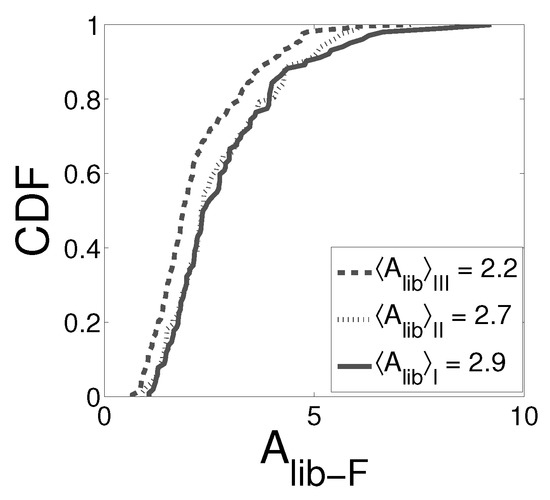
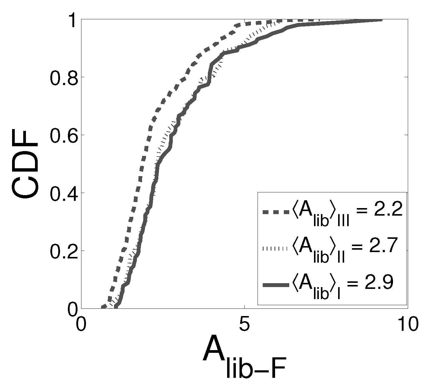
The experiments analyzed here were presented and described in detail in [10]. A description of how they were performed is included in Materials and Methods. In brief, we elicited IP${}_3$-mediated Ca${}^{2+}$ release events in Xenopus laevis oocytes that were previously injected with caged IP${}_3$, the Ca${}^{2+}$ buffer, EGTA, and a fast, Fluo-4, and a slow, Rhod-2, Ca${}^{2+}$ dye. The signals were elicited by uncaging the caged IP${}_3$ with an UV flash. In the current paper, we analyze the changes observed in the distribution of localized Ca${}^{2+}$ release events (puffs) elicited in this way as the concentration of the slow dye, ${\left[R\right]}_T=[Rhod-$2], is varied but all other experimental parameters are kept fixed ($\left[EGTA\right]=90\mathsf{\mu }\mathrm{M}$; $[Fluo-$4${]=\left[F\right]}_T=36\mathsf{\mu }\mathrm{M}$, duration of the UV flash to uncage the IP${}_3$ $=(100-200)$ ms; see Table 1). In particular, we are interested in studying the changes in the “size” of the elicited release events that remain localized (Ca${}^{2+}$ puffs), where by size we mean the number of IP${}_3$Rs that are simultaneously open at the release site (the cluster) during the release event. In order to compare the localized event size distributions obtained in experiments performed for different values of ${\left[R\right]}_T$, we introduced in [10] a quantity, $A_{lib-F}$, that is an increasing function of the Ca${}^{2+}$ current that underlies the observed release event regardless of the value of ${\left[R\right]}_T$. We describe in Section 4.3 how we compute $A_{lib-F}$ from the fluorescence emitted by the Ca${}^{2+}$-bound Fluo-4 molecules. We show in Figure 1 the cumulative distribution functions (CDFs) of $A_{lib-F}$ derived from the experiments performed for the conditions of Set III (dashed line), Set II (dotted line) and Set I (solid line). These CDFs were computed including only localized events, i.e., Ca${}^{2+}$ puffs.

Table 1. Combinations of the dyes and EGTA concentrations used in the different experiments.

Experiment	[Fluo-4] ($\mathsf{\mu }\mathbf{M}$)	[Rhod-2] ($\mathsf{\mu }\mathbf{M}$)	[EGTA] ($\mathsf{\mu }\mathbf{M}$)
Set I	36	90	90
Set II	36	36	90
Set III	36	0	90

Figure 1. CDF of event sizes (as measured by $A_{lib-F}$) for experiments performed with ${\left[F\right]}_T=36\mathsf{\mu }\mathrm{M}$ and $\left[EGTA\right]=90\mathsf{\mu }\mathrm{M}$ and different values of ${\left[R\right]}_T$ (the solid line corresponds to Set I, the dotted line to Set II and the dashed line to Set III (see Table 1).

The Kolmogorov–Smirnov test rejects the null hypothesis that $A_{lib-F}$ from sets III and II and sets III and I come from the same continuous distribution with a 99% significance level ($p_{value}=2.1\times {10}^{-4}$ and $p_{value}=4.6\times {10}^{-5}$, respectively), but cannot reject that the data points from Set II and Set I come from the same distribution ($p_{value}=0.96$). In any case, there is a tail in the CDF of $A_{lib-F}$ for Set I that is unobservable in that of Set II which is consistent with having more events with relatively larger underlying Ca${}^{2+}$ currents in the former than in the latter ($⟨A_{lib-F}⟩=2.2$ for Set III $⟨A_{lib-F}⟩=2.7$ for Set II and $⟨A_{lib-F}⟩=2.9$ for Set I). These comparisons indicate that puffs with relatively larger underlying Ca${}^{2+}$ currents can be elicited as the concentration of the slow dye, Rhod-2, is increased. Although the transformation from puff amplitude to $A_{lib-F}$ involves certain uncertainties, the changes observed in the fluorescence rise time as ${\left[R\right]}_T$ is varied [10] support this conclusion.

2.2. Probabilistic Model to Analyze the Differences Observed in the Experimental Event Size Distributions for Different Values of ${\left[R\right]}_T$

As analyzed in [14], being able to observe localized Ca${}^{2+}$ release events (puffs) with larger Ca${}^{2+}$ currents as a slow buffer concentration (in this case, Rhod-2) is increased can be due to a more efficient uncoupling between IP${}_3$R clusters due to the presence of the slow buffer. Namely, we have the hypothesis that the differences in the CDFs of localized release event sizes illustrated in Figure 1 occur because, as ${\left[R\right]}_T$ decreases, Ca${}^{2+}$ release events with too many simultaneously open IP${}_3$Rs at the primary site can no longer remain localized, induce the opening of IP${}_3$Rs in neighboring (secondary) clusters and, thus, are not included to compute the CDF. We hereby introduce a way to analyze the experimental data to quantify what fraction of events that are localized for a given ${\left[R\right]}_T$ turn into waves as ${\left[R\right]}_T$ is decreased.

We define $P\left(n_c\right)$ as the probability that there are $n_c$ simultaneously open IP${}_3$Rs in a cluster for a given set of experimental conditions. Here, we will assume that all conditions remain the same except for the total slow dye concentration, ${\left[\mathrm{R}\right]}_T$. Thus, we will analyze the change of $P\left(n_c\right)$ with ${\left[\mathrm{R}\right]}_T$. Given that there are $n_c$ simultaneously open IP${}_3$Rs we want to distinguish whether this situation induces the opening of at least one IP${}_3$R in a neighboring (secondary) cluster (i.e., it initiates a wave) or it does not (i.e., the Ca${}^{2+}$ release event due to the $n_c$ simultaneously open IP${}_3$Rs remains localized). We then write:

$$P\left(n_c\right)=P(n_c\&\ell |{\left[\mathrm{R}\right]}_T)+P(n_c\&w|{\left[\mathrm{R}\right]}_T).$$

(1)

In Equation (1), $P(n_c\&\ell |{\left[\mathrm{R}\right]}_T)$ is the joint probability that $n_c$ channels are simultaneously open in a cluster and the event stays localized for a given value of ${\left[\mathrm{R}\right]}_T$. $P(n_c\&w|{\left[\mathrm{R}\right]}_T)$ is the joint probability that $n_c$ channels are simultaneously open in a cluster and the event induces the opening of at least one IP${}_3$R in another cluster for a given value of ${\left[\mathrm{R}\right]}_T$. The symbol | means that these are two conditional probabilities for a given value of the slow dye concentration, ${\left[R\right]}_T$. All the probabilities we work with here are defined over the set of events, i.e., for $n_c\ge 1$. The aim of this calculation is to assess how the two joint probabilities of Equation (1) change with ${\left[R\right]}_T$. Under the assumption that Rhod-2 is a slow buffer and, as such, does not affect CICR within the cluster [14], we consider that $P\left(n_c\right)$ does not depend on ${\left[R\right]}_T$. What may change when varying Rhod-2 is whether the event with $n_c$ open channels in a cluster remains localized (stays as a puff) or elicits the opening of channels in a neighboring cluster (becomes a wave). We rewrite the two joint probabilities of interest as:

$$\begin{array}{ccc}\hfill P(n_c\&\ell |{\left[\mathrm{R}\right]}_T)& =& P\left(n_c\right|\ell ,{\left[\mathrm{R}\right]}_T)P\left(\ell \right|{\left[\mathrm{R}\right]}_T)\hfill \\ & =& P\left(n_c\right|\ell ,{\left[\mathrm{R}\right]}_T)\left(1-P\left(w\right|{\left[\mathrm{R}\right]}_T)\right),\hfill \end{array}$$

(2)

$$\begin{array}{ccc}\hfill P(n_c\&w|{\left[\mathrm{R}\right]}_T)& =& P\left(w\right|n_c,{\left[\mathrm{R}\right]}_T)P\left(n_c\right).\hfill \end{array}$$

(3)

In these equations, $P\left(n_c\right|\ell ,{\left[\mathrm{R}\right]}_T)$ is the probability that a Ca${}^{2+}$ release event that remains localized for a given ${\left[\mathrm{R}\right]}_T$ corresponds to a situation with $n_c$ simultaneously open channels at the release site; $P\left(w\right|n_c,{\left[\mathrm{R}\right]}_T)$ is the probability that, for $n_c$ open channels in a cluster and a given ${\left[\mathrm{R}\right]}_T$, the resulting event induces the release of Ca${}^{2+}$ from a neighboring cluster (i.e., generates a wave). $P\left(\ell \right|n_c,{\left[\mathrm{R}\right]}_T)$ and $P\left(w\right|n_c,{\left[\mathrm{R}\right]}_T)$, on the other hand, are the probabilities that a Ca${}^{2+}$ release event obtained for given ${\left[\mathrm{R}\right]}_T$ remains localized or initiates a wave, respectively. They satisfy: $P\left(\ell \right|n_c,{\left[\mathrm{R}\right]}_T)+P\left(w\right|n_c,{\left[\mathrm{R}\right]}_T)=1$. We rewrite the latter as:

$$P\left(w\right|{\left[\mathrm{R}\right]}_T)=\sum _{n_c\ge 1}P\left(w\right|n_c,{\left[\mathrm{R}\right]}_T)P\left(n_c\right).$$

(4)

Combining Equations (1)–(3), we arrive at:

$$\begin{array}{ccc}\hfill P\left(n_c\right)& =& P\left(n_c\right|\ell ,{\left[\mathrm{R}\right]}_T)\left(1-P\left(w\right|{\left[\mathrm{R}\right]}_T)\right)\hfill \\ & +& P\left(w\right|n_c,{\left[\mathrm{R}\right]}_T)P\left(n_c\right).\hfill \end{array}$$

(5)

Assuming that the Ca${}^{2+}$ current through an open IP${}_3$R is approximately the same for all IP${}_3$Rs, we conclude that $n_c$ is proportional to the Ca${}^{2+}$ current that underlies a Ca${}^{2+}$ release event. The quantity $A_{lib-F}$ that we derive from the experimental data, on the other hand, is an increasing function of the underlying Ca${}^{2+}$ current. We must point out that, if $n_c$ is large enough, puff amplitudes increase sublinearly with $n_c$ [15]. Assuming that $n_c$ and $A_{lib-F}$ are approximately linearly related, we can then use the experimental CDF of $A_{lib-F}$, which we compute for the localized Ca${}^{2+}$ release events, to estimate the CDF, F that can be computed from $P\left(n_c\right|\ell ,{\left[\mathrm{R}\right]}_T)$:

$$\begin{array}{c}\hfill F(n,|\ell ,{\left[R\right]}_T)=\sum _{n_c=1}^{n}P\left(n_c\right|\ell ,{\left[R\right]}_T).\end{array}$$

(6)

The aim is to compare the distribution functions, $F(n,|\ell ,{\left[R\right]}_T)$, for different values of ${\left[R\right]}_T$ using the corresponding experimental CDFs of $A_{lib-F}$. In particular, we will compare the CDFs that are sufficiently different according to the K–S test: the ones with ${\left[R\right]}_T=0$ and with ${\left[R\right]}_T=90\mathsf{\mu }\mathrm{M}$. In what follows, we will drop the concentration units ($\mathsf{\mu }\mathrm{M}$) from the expressions of the probabilities to simplify the notation. Defining $∆P_w\left(n_c\right)\equiv P\left(w\right|n_c,0)-P\left(w\right|n_c,90)$ and $∆P_w\equiv {\sum }_{n_c\ge 1}∆P_w\left(n_c\right)P\left(n_c\right)$ and using Equations (4) and (5), we obtain:

$$∆P_w\left(n_c\right)P\left(n_c\right)=\left(P\left(n_c\right|\ell ,90)-P\left(n_c\right|\ell ,0)\right)(1-P\left(w\right|90))+P\left(n_c\right|\ell ,0)∆P_w.$$

(7)

As illustrated in Figure 1, the experiments show that the difference between the two CDFs is more noticeable in the region of the largest size events, i.e., for the largest values of $n_c$. We then compute:

$$\sum _{n_c\ge n_M}∆P_w\left(n_c\right)P\left(n_c\right)=\left(F\left(n_M\right|\ell ,0)-F\left(n_M\right|\ell ,90)\right)(1-P\left(w\right|90))+∆P_w(1-F\left(n_M\right|\ell ,0)),$$

(8)

where $n_M$ is the event size beyond which the CDFs start to differ more noticeably. As described later, the CDFs in the r.h.s. of Equation (8) can be estimated from the experimental CDFs. On the other hand, we estimate $P\left(w\right|n_c,{\left[\mathrm{R}\right]}_T)$ using the numerical simulations that we describe in the following section. Varying the parameters of the simulation, we determine the values for which we obtain estimates of the l.h.s. of this equation that are consistent with those of the r.h.s.

2.3. Numerical Simulations to Estimate the Probability That a Release Event from One (Primary) Cluster Induces the Release of Ca${}^{2+}$ from Another (Secondary) Cluster

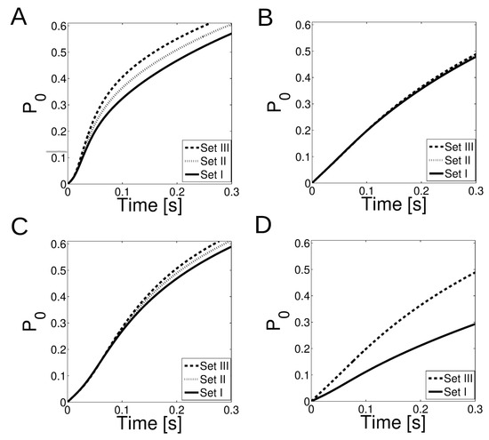
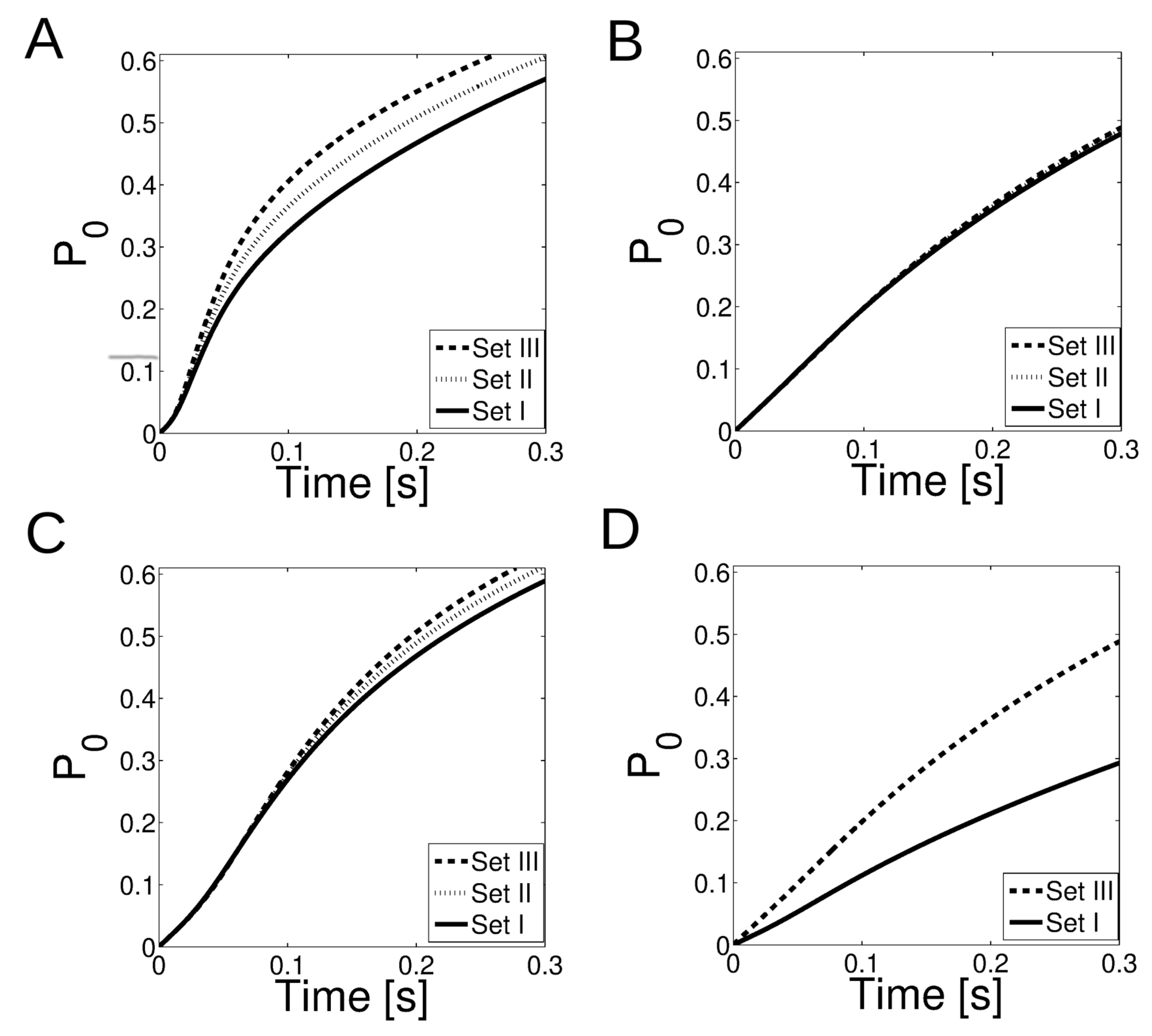
We compute the probability, $P_0(t,d,n_c,n_s,{\left[R\right]}_T),$ that $n_s$ IP${}_3$R located at a distance, d, from a (primary) cluster with $n_c$ IP${}_3$Rs that are simultaneously open at $t=0$, becomes open by a time, t. We want to compare how $P_0$ varies as ${\left[R\right]}_T$ is changed. We thus write explicitly its dependence on this variable. To compute $P_0(t,d,n_c,n_s,{\left[R\right]}_T)$, we proceed as explained in Materials and Methods (see also [10]) and the parameter values used are listed in Table 2. We show in Figure 2 the results obtained with $n_s=1$. We show in Figs. Figure 2a–c the results obtained using the basal Ca${}^{2+}$ concentration, [Ca]${}_b$ = $0.1\mathsf{\mu }\mathrm{M}$, for the conditions of Sets I, II and III. We show the results obtained at $d=0.6\mathsf{\mu }\mathrm{m}$ in Figure 2a and at $d=1.4\mathsf{\mu }\mathrm{m}$ (a typical inter-cluster distance) in Figure 2b,c. The number of simultaneously open channels is $n_c=10$ in Figure 2a,b and $n_c=50$ in Figure 2c. The change of $P_0$ with varying ${\left[R\right]}_T$ is unobservable for $n_c=10$ at $d=1.4\mathsf{\mu }\mathrm{m}$ (the difference is $\le 0.004$ for the times displayed in the figure) while it can be $\sim 0.085$ at $d=0.6\mathsf{\mu }\mathrm{m}$. Furthermore, it is $∆P_0\left(t\right)=P_0(t,d=0.6\mathsf{\mu }\mathrm{m},n_c=10,{\left[R\right]}_T=90\mathsf{\mu }\mathrm{M})-P_0(t,d=0.6\mathsf{\mu }\mathrm{m},n_c=10,{\left[R\right]}_T=0\mathsf{\mu }\mathrm{M})\approx 0.065$ at $t=d/V$ with $V\sim 10\mathsf{\mu }{\mathrm{ms}}^{-1}$, a typical wave velocity. The maximum difference ${max}_t∆P_0\left(t\right)$ increases with $n_c$. This is shown in Figure 2c where $n_c=50$, $d=1.4\mathsf{\mu }\mathrm{m}$ and ${max}_t∆P_0\left(t\right)\sim 0.026$. In Figure 2d, we show what happens when [Ca]${}_b$ decreases. In this case, we compare $P_0$ at a distance $d=1.4\mathsf{\mu }\mathrm{m}$ from the source obtained for simulations performed with the concentrations of Set III (dashed line) and Set I (solid line) but with a different value of [Ca]${}_b$ in each one (100 nM and 50 nM, respectively). A similar behaviour is obtained with $n_s=5$ (data not shown).

Table 2. Value of the parameters varied to compute $P_0$.

Parameter	Abbreviature	Values
Number of IP${}_3$Rs in the source	$n_c$	1, 10, 50
Distance to the Ca${}^{2+}$ source	d	(0.4–1.5) $\mathsf{\mu }$m
Number of sensing IP${}_3$Rs	$n_s$	1, 5
Rhod-2 concentration	${\left[R\right]}_T$	0, 90 $\mathsf{\mu }$M
Velocity of propagation	V	10, 20 $\mathsf{\mu }$m/s

Figure 2. $P_0$ dependence with distance d from the source and [Ca]${}_b$. (a) performed at $d=0.6\mathsf{\mu }\mathrm{m}$ with $n_c=10$; (b) at $d=1.4\mathsf{\mu }\mathrm{m}$ with $n_c=10$; (c) at $d=1.4\mathsf{\mu }\mathrm{m}$ and $n_c=50$ and (d) $d=1.4\mathsf{\mu }\mathrm{m}$ with $n_c=10$ while varying [Ca]${}_b$ from 100 nM (Set III) to 50 nM (Set I). The dashed line corresponds to Set III, the dotted line corresponds to Set II, and the solid line corresponds to Set I.

We interpret the ${\left[R\right]}_T$-dependent changes of $P_0$ that are illustrated in Figure 2 as a sign of the change in the level of inter-cluster coupling (or, equivalently, disruption) that can be reached as the slow dye concentration is varied.

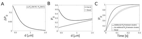
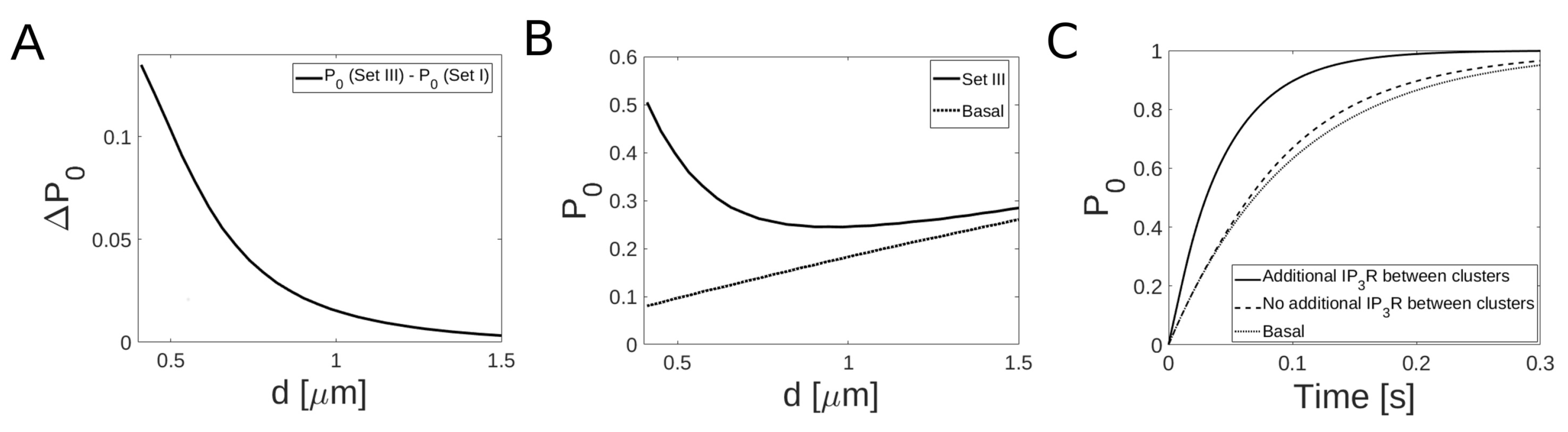
We further studied how sensitive is $P_0$ to changes in the distance to the source d. The results of Figure 3 are obtained using the basal Ca${}^{2+}$ concentration, [Ca]${}_b$ = $0.1\mathsf{\mu }\mathrm{M}$. To illustrate the disruption when ${\left[R\right]}_T$ is increased, we show in Figure 3a $∆P_0=P_0({\left[R\right]}_T=0)-P_0({\left[R\right]}_T=90\mathsf{\mu }\mathrm{M})$ computed with $n_c=10$ and $n_s=1$ as a function of the distance d for each time $t=d/V$ (with $V=10\mathsf{\mu }\mathrm{m}/\mathrm{s}$) and it can be observed that the probability of opening one IP${}_3$R in-between clusters decreases (from 0.4 $\mathsf{\mu }\mathrm{m}$ to 1.5 $\mathsf{\mu }\mathrm{m}$). When observing the probability of opening one IP${}_3$R as a function of d without adding the slow buffer ($R_T=0$, Set III) (solid line in Figure 3b), as d increases, this probability approximates to the basal probability (dotted line, $P_0$ computed as in Equation (14) but with no calcium dyes), almost no coupling can occur at the typical inter-cluster distance ($d=1.4\mathsf{\mu }\mathrm{m}$). Thus, to explain the inter-cluster coupling, it is necessary to add a non-cluster IP${}_3$R in-between them. The optimal value of the parameter d should be on the order of 0.4–0.8 $\mathsf{\mu }\mathrm{m}$ (approximately the half distance between clusters). Not even adding $n_s=5$ sensing channels at the second cluster, the probability differs from the basal (dashed and dotted lines in Figure 3c, respectively). We choose $d=0.6\mathsf{\mu }\mathrm{m}$ to add an isolated IP${}_3$R in-between clusters (solid line in Figure 3c) and now the signal can propagate.

Figure 3. Existence of IP${}_3$Rs in-between clusters is necessary to explain the observations. (a) $∆P_0=P_0({\left[R\right]}_T=0)-P_0({\left[R\right]}_T=90\mathsf{\mu }\mathrm{M})$ with $n_c=10$ and $n_s=1$ as a function of the distance d for each time $t=d/V$ (with $V=10\mathsf{\mu }\mathrm{m}/\mathrm{s}$); (b) $P_0$ computed as in (a) for the Set III (solid line) and basal (dotted line) conditions; (c) $P_0$ computed in the condition of Set III with $n_c=10$ and $n_s=5$ at a distance $d=1.4\mathsf{\mu }\mathrm{m}$ from the Ca${}^{2+}$ point source as a function of time when an IP${}_3$R is added in-between cluster (solid line), with no additional IP${}_3$R (dashed line) and at the basal condition (dotted lined).

We now study whether the variations of Figure 2 can explain the changes in the distributions of Ca${}^{2+}$ release during localized events observed in the experiments that are apparent in Figure 1.

2.4. Combining the Estimates Derived from the Experiments and from the Numerical Simulations to Interpret the Changes Observed Experimentally

We first estimate the r.h.s. of Equation (8) assuming that $F(n,|\ell ,{\left[R\right]}_T)$ is given by the experimental CDF of $A_{lib-F}$ for the same ${\left[R\right]}_T$ and some unknown factor between n and $A_{lib-F}$. We recall here that the experimental CDF corresponds only to localized events (i.e., events at a primary cluster that do not induce the opening of IP${}_3$Rs at another secondary IP${}_3$R cluster). In order to estimate this unknown factor, we associate, $n_M$, (the value after which the differences in the CDFs become more noticeable) to a value, $A_{lib-F}$, for which $F\left(n_M\right|\ell ,0)$ is sufficiently close to 1. The basic assumption here is that, for ${\left[R\right]}_T=0$, almost all primary events with $n\le n_M$ simultaneously open IP${}_3$Rs initiate waves in which case they do not remain localized and are, therefore, not included in the computation of the CDF. We choose $A_{lib-F}=4.8$ for which, according to the experimental data, it is $F\left(n_M\right|\ell ,0)\approx 0.98$ (see Figure 1). For this value, it is $F\left(n_M|\ell ,90)\right)\approx 0.90$. Thus, we estimate $F\left(n_M\right|\ell ,0)-F\left(n_M\right|\ell ,90)\approx 0.08$. We do not have a direct estimation of $P\left(w\right|{\left[\mathrm{R}\right]}_T)$. Assuming that $n_c=10$ is the most probable value for the number of simultaneously open IP${}_3$Rs in a cluster, we approximate $P\left(w\right|{\left[R\right]}_T)={\sum }_{n_c\ge 1}P\left(w\right|n_c,{\left[\mathrm{R}\right]}_T)P\left(n_c\right)\approx P\left(w\right|n_c=10,{\left[\mathrm{R}\right]}_T)\approx P_0(t=d/V,d,n_c=10,{\left[R\right]}_T)$ with $P_0$ the open probability computed numerically that we introduced in the previous section and V a typical Ca${}^{2+}$ wave velocity. For V, we try two values, $V=20\mathsf{\mu }\mathrm{m}/\mathrm{s}$ and $V=10\mathsf{\mu }\mathrm{m}/\mathrm{s}$. For d, we try the typical inter-cluster distance, $d=1.4\mathsf{\mu }\mathrm{m}$ and the closer distance, $d=0.6\mathsf{\mu }\mathrm{m}$ that was probed in the previous section. Using $d=1.4\mathsf{\mu }\mathrm{m}$ and $V=20\mathsf{\mu }\mathrm{m}/\mathrm{s}$, the simulations give $P\left(w\right|90)\approx 0.14$ and $∆P_w\approx 0$. The estimate of the r.h.s. of Equation (8) then results equal to $0.07$. This value changes to $0.06$ if we use $V=10\mathsf{\mu }\mathrm{m}/\mathrm{s}$. Using $d=0.6\mathsf{\mu }\mathrm{m}$ and $V=20\mathsf{\mu }\mathrm{m}/\mathrm{s}$ the simulations give $P\left(w\right|90)\approx 0.12$ and $∆P_w=0.028$. The estimate of the r.h.s. of Equation (8) then results as $0.07$. This value changes to $0.06$ if we use $V=10\mathsf{\mu }\mathrm{m}/\mathrm{s}$.

We now use the simulations of the previous section to put an upper bound, $∆P_{w,max}$, on $∆P_w\left(n_c\right)$ in the l.h.s of Equation (8). With such an upper bound, we can write ${\sum }_{n_c\ge n_M}∆P_w\left(n_c\right)P\left(n_c\right)\le ∆P_{w,max}{\sum }_{n_c\ge n_M}P\left(n_c\right)=∆P_{w,max}(1-F\left(n_M\right))$ where $F\left(n_M\right)={\sum }_{n_c\le n_M}P\left(n_c\right)$. Similarly to the way we have followed estimating $P\left(w\right|{\left[R\right]}_T)$, we compute $P\left(w\right|n_c,{\left[R\right]}_T)\approx P_0(t=d/V,d,n_c,{\left[R\right]}_T)$, with $P_0$ the open probability of the previous section illustrated in Figure 2. In particular, using the results of these simulations, we conclude that $∆P_w\left(n_c\right)\equiv P\left(w\right|n_c,0)-P\left(w\right|n_c,90\mathsf{\mu }\mathrm{M})$ is larger the larger the value of $n_c$. Thus, we obtain the upper bound, $∆P_{w,max}$, using similar simulations to those of Figure 2 but for $n_c=50$ (a very large number of simultaneously open IP${}_3$Rs). Namely, we estimate $∆P_{w,max}\approx P_0(t=d/V,d,n_c=50,0)-P_0(t=d/V,d,n_c=50,90)$. In order to put an upper bound on the l.h.s. of Equation (8), we need a bound for $F\left(n_M\right)$, the CDF of all the (primary) event sizes at $n=n_M$. As already explained, we assume that $F\left(n\right)={\sum }_{n_c\le n}P\left(n_c\right)$ does not depend on ${\left[R\right]}_T$. Given our interpretation of the results, we assume that the difference between the CDF of all the (primary) event sizes, $F\left(n\right)$, and the CDF of the primary event sizes that remain localized for a given value of ${\left[R\right]}_T$, $F\left({n|\ell ,\left[R\right]}_T\right)$, is due to the existence of primary events (of large enough size) that initiate waves for that value of ${\left[R\right]}_T$. Assuming that the fraction of primary events that initiate waves for ${\left[R\right]}_T=90\mathsf{\mu }M$ is negligible, we can approximate $F\left(n_M\right)\approx F\left(n_M|\ell ,90\right)\approx 0.90$. If we do not want to use this approximation, then we can use the bound $F\left(n_M\right)<0.90$. In what follows, we mostly use $F\left(n_M\right)=0.90$, but we repeat some computations changing it to 0.80 to see how much the estimates could change. Proceeding as just explained, for $d=1.4\mathsf{\mu }\mathrm{m}$, we obtain $∆P_w\left(n_c\right)\le ∆P_{w,max}\approx 0.003$ for $V=20\mathsf{\mu }\mathrm{m}/\mathrm{s}$ and $∆P_{w,max}\approx 0.026$ for $V=10\mathsf{\mu }\mathrm{m}/\mathrm{s}$. Using $F\left(n_M\right)=0.9$, we then obtain $\sim 0.0003$ and $0.0026$ as upper bounds of the l.h.s. of Equation (8) for $V=20\mathsf{\mu }\mathrm{m}/\mathrm{s}$ and $V=10\mathsf{\mu }\mathrm{m}/\mathrm{s}$, respectively. These two upper bounds are at least one order of magnitude smaller than the values obtained for the r.h.s. of Equation (8). If we use $F\left(n_M\right)=0.8$ to compute the l.h.s. of this equation, the latter estimate doubles with respect to the previous one. Thus, the order of magnitude difference between the left and right estimates for $d=1.4\mathsf{\mu }\mathrm{m}$ remains the same. Repeating the computations for $d=0.6\mathsf{\mu }\mathrm{m}$, we obtain $∆P_w\left(n_c\right)\le ∆P_{w,max}\approx 0.19$ for $V=20\mathsf{\mu }\mathrm{m}/\mathrm{s}$ and $∆P_{w,max}\approx 0.15$ for $V=10\mathsf{\mu }\mathrm{m}/\mathrm{s}$. Using $F\left(n_M\right)=0.9$, we then get $\sim 0.019$ and $0.015$ as upper bounds of the l.h.s. of Equation (8) for $V=20\mathsf{\mu }\mathrm{m}/\mathrm{s}$ and $V=10\mathsf{\mu }\mathrm{m}/\mathrm{s}$, respectively. In this case, the values of the left- and right-hand sides are of the same order of magnitude. These estimates come closer together if we use $F\left(n_M\right)=0.8$ in the l.h.s. of the equation. In such a case, we obtain $\sim 0.04$ and $\sim 0.03$ for the l.h.s. estimate using $V=20\mathsf{\mu }\mathrm{m}/\mathrm{s}$ and $V=10\mathsf{\mu }\mathrm{m}/\mathrm{s}$, respectively, two values that are pretty similar to the r.h.s. estimates, 0.07 and 0.06.

2.5. Changes in Basal Calcium Concentration, [Ca]${}_b$

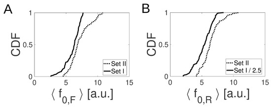
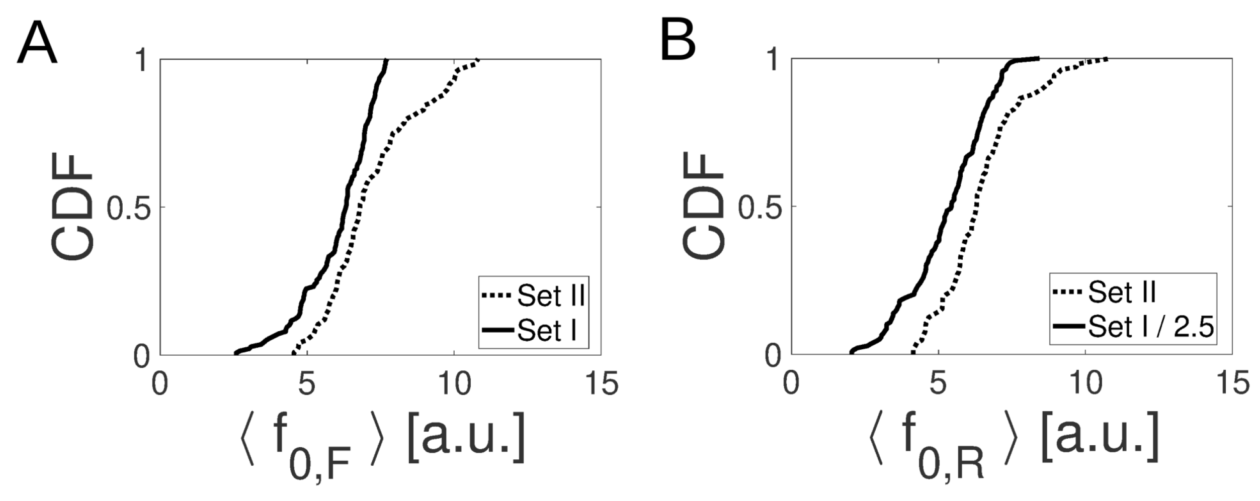
As illustrated in Figure 2d, decreasing basal [Ca] with increasing ${\left[R\right]}_T$ changes the open probability at the distance, $d=1.4\mathsf{\mu }\mathrm{m}$, in the direction that is needed to explain the observed changes in the event size distributions. We analyze here whether there is any evidence of a decreasing basal Ca${}^{2+}$ with increasing ${\left[R\right]}_T$ in the experimental data. We show in Figure 4 the cumulative density functions of the mean basal fluorescence emitted by the Ca${}^{2+}$-bound Fluo-4 molecules, $⟨f_{0,F}⟩$, in (a) and of the mean basal fluorescence emitted by the Ca${}^{2+}$-bound Rhod-2 molecules, $⟨f_{0,R}⟩$ in (b) for the experiments with ${\left[R\right]}_T=36\mathsf{\mu }\mathrm{M}$ (dotted line) and with ${\left[R\right]}_T=90\mathsf{\mu }\mathrm{M}$ (solid line). In Figure 4b, we rescaled $⟨f_{0_R}⟩$ by $90/36=2.5$ in the case of Set I to make the distributions of experiments of Set I (which has ${\left[R\right]}_T=90\mathsf{\mu }\mathrm{M}$) and II (which has ${\left[R\right]}_T=36\mathsf{\mu }\mathrm{M}$) readily comparable. The values of $⟨f_{0,F}⟩$ and $⟨f_{0,R}⟩$ were derived from the fluorescence observations as explained in Materials and Methods. We observe that the CDFs move to smaller values of their arguments with increasing ${\left[R\right]}_T$. As the mean basal fluorescence is an increasing function of [Ca]${}_b$ (see Equation (12)), this observation supports the idea that, on average, [Ca]${}_b$ decreases with increasing Rhod-2.

Figure 4. CDF of basal fluorescence. $⟨f_{0,D}⟩$ for experiments with $\left[EGTA\right]=90\mathsf{\mu }\mathrm{M}$ are shown in the Fluo-4 ($D=F$, (a)) and Rhod-2 ($D=R$, (b)) channels. In both cases, Set II is depicted with dotted lines and Set I with solid lines. In (b), the values, $⟨f_{0,R}⟩$, of Set I are divided by $90/36=2.5$ to make both distributions comparable.

In order to estimate the variation in [Ca]${}_b$ with increasing ${\left[R\right]}_T$, we compare $\overline{⟨f_{0,D}⟩}$ for sets I and II. In particular, we obtain $\overline{⟨f_{0,F}⟩}$ = 6.1 a.u., $\overline{⟨f_{0,R}⟩}$ = 13.2 a.u. and $\overline{⟨f_{0,F}⟩}$ = 7.2 a.u., $\overline{⟨f_{0,R}⟩}$ = 6.4 a.u. for sets I and II, respectively. Inserting these values into Equation (13), using that $⟨N_R⟩=32$ for set II and $⟨N_R⟩=80$ for set I, and assuming that [Ca]${}_b$ = 100 nM for set II, we obtain [Ca]${}_b$ = 60–80 nM for set I, depending on whether we use the mean Rhod-2 or mean Fluo-4 basal fluorescence values.

We now repeat the calculations of the previous section but using the values of $P_0$ prescribed by the simulations with [Ca]${}_b$ = 100 nM for set II and [Ca]${}_b$ = 50 nM for set I (Figure 2d). In this case, the r.h.s. estimates do not change much from the previous calculations. The l.h.s. estimates, on the other hand, change slightly coming closer together with the r.h.s. estimates. For example, using $V=20\mathsf{\mu }\mathrm{m}/\mathrm{s}$, we obtain l.h.s. $\approx 0.023$ for $d=0.6\mathsf{\mu }\mathrm{m}$ and l.h.s. $\approx 0.007$ for $d=1.4\mathsf{\mu }\mathrm{m}$. If we use $V=10\mathsf{\mu }\mathrm{m}/\mathrm{s}$, we obtain l.h.s. $\approx 0.019$ for $d=0.6\mathsf{\mu }\mathrm{m}$ and l.h.s. $\approx 0.013$ for $d=1.4\mathsf{\mu }\mathrm{m}$.

3. Discussion

Intracellular Ca${}^{2+}$ signals are ubiquitous across cell types. The spatial range over which they spread is key to determining the eventual end responses. This points to the importance of understanding how intracellular Ca${}^{2+}$ signals propagate inside the cells. To this end, Ca${}^{2+}$ release from the endoplasmic reticulum into the cytosol through IP${}_3$Rs plays a major role. IP${}_3$Rs are Ca${}^{2+}$ channels whose open probability depends on the cytosolic Ca${}^{2+}$ concentration. Therefore, the Ca${}^{2+}$ released through an open IP${}_3$R can induce the opening of nearby IP${}_3$Rs. High Ca${}^{2+}$ concentrations, on the other hand, lead to the inhibition of the channels. This dynamic is clearly excitable. In this regard, however, the excitability of the cytosol is “patchy”: IP${}_3$Rs tend to be organized in clusters separated by $\sim 1.4\mathsf{\mu }\mathrm{m}$. This may lead to propagation failure when the Ca${}^{2+}$ released from one IP${}_3$R reaches the vicinity of another one at a concentration that is not enough to induce its opening. The inter-cluster Ca${}^{2+}$-mediated coupling can be interfered by means of Ca${}^{2+}$ buffers. This is used as an experimental tool, but the cells can do it as well.

In [10], we presented experimental results in which we studied how the presence of competing Ca${}^{2+}$ trapping mechanisms of different kinetics altered the resulting intracellular signals. Differently from previous studies [12], in [10], we made visible the invisible by using two dyes of different kinetics as the Ca${}^{2+}$ trapping mechanisms. The work of [10] not only allowed us to draw conclusions on how the signals were reshaped by the presence of the different buffers but also gave some indications on the spatial distribution of the IP${}_3$Rs involved in the signals. In particular, based on a qualitative comparison between experiments and numerical simulations, we concluded in [10] that Ca${}^{2+}$ release seemed to occur not only from the clearly identifiable release sites (IP${}_3$R clusters), but also from some functional, probably isolated, IP${}_3$Rs in between them. In this paper, we have presented a quantitative analysis of the experiments of [10] that corroborated this conclusion.

For the quantitative comparison between experiments and models, in this paper, we have focused on the size distribution of the localized Ca${}^{2+}$ release events (puffs) that were obtained with the experiments of [10] for $\left[EGTA\right]=90\mathsf{\mu }\mathrm{M}$, ${\left[F\right]}_T=36\mathsf{\mu }\mathrm{M}$ and two concentrations of the slow dye Rhod-2, ${\left[R\right]}_T=36\mathsf{\mu }\mathrm{M}$ and $90\mathsf{\mu }\mathrm{M}$. Given that the fluorescence amplitude observed for a given release event could change with varying ${\left[R\right]}_T$ even if the underlying Ca${}^{2+}$ current remained the same, we characterized the observed puffs by the quantity, $A_{lib-F}$ (Equation (11)) that we introduced in [10] to overcome this problem. The $A_{lib-F}$ distributions obtained for the analyzed experiments showed a shift towards larger values of $A_{lib-F}$ as ${\left[R\right]}_T$ was increased (see Figure 1). This shift agrees with previous observations and analyses according to which the increase of a slow Ca${}^{2+}$ buffer concentration (in this case, Rhod-2) disrupts the Ca${}^{2+}$-mediated coupling between clusters (Figure 3a) [10,12,14,16]. Namely, we interpret this shift as reflecting the fact that events that are characterized by a certain number of simultaneously open IP${}_3$Rs at a primary cluster and remain localized for a given value of ${\left[R\right]}_T$ can induce the opening of IP${}_3$Rs at other (secondary) clusters for smaller values of ${\left[R\right]}_T$. While the former events are puffs and would then be considered for the computation of the localized event size distribution, the latter would not because they correspond to waves.

We observed that clusters can become coupled when adding an IP${}_3$R in-between them (Figure 3c). We introduced a probabilistic model in order to analyze quantitatively whether the differences observed for the experiments performed for ${\left[R\right]}_T=0$ and ${\left[R\right]}_T=90\mathsf{\mu }\mathrm{M}$ could be explained if Ca${}^{2+}$ release only occurred through IP${}_3$R-clusters separated by 1.4 $\mathsf{\mu }\mathrm{m}$ or not. Within the framework of the probabilistic model, we then combined the analysis of the experimental data with some probability estimates derived from numerical simulations similar to those presented in [10]. We determined in this way that the numerically estimated values were not compatible with the differences observed experimentally if the only Ca${}^{2+}$ release sites involved were $\sim 1.4\mathsf{\mu }\mathrm{m}$ apart from one another. The experimental and numerical results were more compatible if we assumed that there was Ca${}^{2+}$ release from at least one IP${}_3$R at a distance $\sim 0.6\mathsf{\mu }\mathrm{m}$ from the primary Ca${}^{2+}$ release cluster. The presence of the slow dye, on the other hand, could reduce the basal Ca${}^{2+}$ concentration. We analyzed that possibility in the experimental data (Figure 4) and estimated that [Ca]${}_b$ could have been reduced by half when ${\left[R\right]}_T$ was changed from 0 to 90 $\mathsf{\mu }\mathrm{M}$. The numerical simulations, on the other hand, showed that a decreasing value of [Ca]${}_b$ with increasing ${\left[R\right]}_T$ gave better results for $d=1.4\mathsf{\mu }\mathrm{m}$ (Figure 2d) in terms of their compatibility with their experiments. We then re-analyzed the experimental data but using numerical simulations that included this change in [Ca]${}_b$ with varying ${\left[R\right]}_T$. The best situation to explain Figure 1 was obtained with simulations that combined a change in [Ca]${}_b$ with ${\left[R\right]}_T$ and the presence of a functional IP${}_3$R at a shorter distance ($d\sim 0.6\mathsf{\mu }\mathrm{m}$) than the typical inter-cluster one.

Our quantitative analysis of the experiments of [10] presented in this paper confirms that the spatial landscape over which intracellular Ca${}^{2+}$ signals propagate do not consist solely of patches of excitability that are 1.4–2 $\mathsf{\mu }\mathrm{m}$ apart from one another but that there are also “relay stations” (isolated functional IP${}_3$Rs) in between. Probably, the existence of these in-between IP${}_3$Rs is necessary for the propagation of Ca${}^{2+}$ waves.

4. Materials and Methods

4.1. Oocyte Preparation

Experiments were performed on Xenopus laevis immature oocytes previously treated with collagenase. Oocytes were loaded by intracellular microinjection with different compounds. Two calcium dyes Fluo-4 dextran high affinity ($K_d=0.8\mathsf{\mu }\mathrm{M}$) and Rhod-2 ($K_d=2\mathsf{\mu }\mathrm{M}$) were used to probe cytosolic [Ca]. Caged InsP${}_3$ (D-Myo-Inositol 1,4,5-Triphosphate,P4(5)-(1-(2-Nitrophenyl)ethyl) Ester) was used to induce IP${}_3$R opening. The exogenous Ca${}^{2+}$ buffer EGTA was also used. Final intracellular concentrations of the different compounds were calculated assuming a 1 $\mathsf{\mu }$L cytosolic volume. Final intracellular concentration of InsP${}_3$ was 9 $\mathsf{\mu }$M in all of the experiments. The different concentrations used in each experiment are detailed in Table 1 where we classify the experiments in three sets. Fluo-4, Rhod-2 and InsP${}_3$ were from Molecular Probes Inc.; EGTA was from Sigma Aldrich. Recordings were made at room temperature.

4.2. Confocal Microscopy

Confocal imaging was performed using a spectral confocal scanning microscope Olympus FluoView1000 that has a spectral scan unit connected to an inverted microscope IX81. The caged compound was photolyzed with the UV part of the spectrum of a mercury lamp that comes with the microscope using the modification introduced in [17]. Fluo-4 was excited with the 488 nm line of a multiline Argon laser, Rhod-2 was excited using the 543 nm line of a He–Ne laser. Both lasers were focused on the oocyte with a $60\times$ oil immersion objective (NA 1.35). The Fluo-4 and Rhod-2 emitted fluorescences were simultaneously detected in the 500–600 nm and the 600–630 ranges, respectively, with PMT detectors. All the experiments were performed in the linescan imaging mode to improve the temporal resolution. Linescan images were obtained by scanning along a fixed line (250 px) within the oocyte. The acquisition rate was fixed at 10 $\mathsf{\mu }$s per pixel resulting in a scan rate of 3.26 ms per line. The caged compound was photo-released approximately 3 s after the linescan acquisition started.

4.3. Image Analysis

All images were analyzed using routines written in MATLAB. In the experiments where we simultaneously acquired the fluorescence coming from two channels (around 510 nm for Fluo-4 and 570 nm for Rhod-2), we used a linear unmmixing method to minimize the effect of the spectral bleed-through ($R=0.1626$ was the linear unmixing coefficient used). The images were also smoothed by averaging over the eight nearest pixels.

The events were identified and the images were processed as explained in [10]. From the fluorescence distribution, $f_D(x_i,t_j)$, collected in each of the channels ($D=R$ for Rhod-2 and $D=F$ for Fluo-4) at each pixel, $(x_i,t_j)$, and the relative increase in fluorescence at the peak of the signal, $∆f_{r,D}={max}_{x_i,tj}((f_{r,D}(x_i,t_j)-f_{0,D}\left(x_i\right))/f_{0,D}\left(x_i\right))$, with $f_{0,D}\left(x_i\right)$ the mean basal fluorescence at $x_i$ observed with D before the UV flash, we computed the corresponding Ca${}^{2+}$-bound dye and (maximum) relative Ca${}^{2+}$ bound dye concentrations ($\left[CaD\right]$ and $∆{\left[CaD\right]}_r\equiv max(\left[CaD\right]-{\left[CaD\right]}_b)/{\left[CaD\right]}_b$, respectively, with ${\left[CaD\right]}_b$ the basal Ca${}^{2+}$-bound dye concentration). To estimate the Ca${}^{2+}$-bound dye concentration, we followed [18] neglecting fluctuations in the number of dye molecules that contribute to the fluorescence at each pixel, $N_D$, (for more details, see [10]):

$$\left[CaD\right]=\frac{{\left[D\right]}_T}{q_{1,D}-q_{2,D}}\left(\frac{f_D}{\gamma ⟨N_D⟩}-q_{2,D}\right),D=R,F,$$

(9)

$$∆{\left[CaD\right]}_r=∆f_{r,D}\left(1+\frac{q_{2,D}/q_{1,D}}{(1-\frac{q_{2,D}}{q_{1,D}})\frac{{\left[Ca\right]}_b}{{\left[Ca\right]}_b+K_{d,D}}}\right),D=R,F.$$

(10)

To compute these quantities we followed [18] and used $⟨N_F⟩=32$, $⟨N_R⟩=32$ for ${\left[R\right]}_T=36\mathsf{\mu }\mathrm{M}$, $⟨N_R⟩=80$ for ${\left[R\right]}_T=90\mathsf{\mu }\mathrm{M}$, [Ca]${}_b$ $=100\mathrm{nM}$, $q_{1,F}=0.45$, $q_{2,F}=0.01$, $K_{d,F}=0.8\mathsf{\mu }\mathrm{M}$, $q_{1,R}=0.36$, $q_{2,R}=0.02$ and $K_{d,R}=2\mathsf{\mu }\mathrm{M}$.

In this paper, we only analyzed the events observed in the Fluo-4 channel, i.e., for $D=F$. The event size of each analyzed puff was then characterized by the maximum value of the relative increase in the Ca${}^{2+}$-bound Fluo-4 concentration, $∆{\left[CaF\right]}_r$ that we derived from the observed fluorescence. As done in [10], we then used the total Rhod-2 concentration, ${\left[R\right]}_T$, of the experiment to obtain estimates of the maximum values, $∆{\left[CaF\right]}_r(\left[R\right]=0)$, that would have been attained for the same release event if only the dye, Fluo-4, had been present. As discussed in [10], this estimate that we call $A_{lib-F}$ is an increasing function of the Ca${}^{2+}$ current that underlies the release event regardless of the value of ${\left[R\right]}_T$ used if the Ca${}^{2+}$ current arises from a very localized spatial region (the cluster). As done in [10], we computed it as:

$$\begin{array}{ccc}\hfill A_{lib-F}& \approx & ∆{\left[CaF\right]}_r+{\alpha }_{F,R}{\left[R\right]}_T,\hfill \\ \hfill \end{array}$$

(11)

with ${\alpha }_{F,R}=4.58\times {10}^{-3}$.

4.4. Basal Calcium Estimation

In order to study the behavior of the mean basal Ca${}^{2+}$ concentration, ${\left[Ca\right]}_b$, for each experiment type probed in the paper, we follow some of the steps of the method introduced in [18]. We work with linescan images obtained before any UV flash has been applied, i.e., we analyze basal fluorescence. On these images, we get rid of the horizontal lines that are persistently dark, which correspond to the cortical granules. We then compute the mean basal fluorescence for each linescan image as:

$$⟨f_{0,D}⟩=\frac{1}{N}\sum _{i\in bf}\sum _{j=1}^{j_{UV}}{f}_D(x_i,t_j),D=R,F,$$

(12)

where the sum over i runs over the horizontal lines that are not persistently dark and the subscript, D, denotes whether the fluorescence comes from the Fluo-4 ($D=F$) or Rhod-2 ($D=R$) molecules. Using the values, $⟨f_{0,D}⟩$, obtained for each experiment type, we compute the corresponding cumulative distribution functions of the mean basal fluorescence. To transform from basal fluorescence to basal Ca${}^{2+}$, we use the following expression derived from [18]:

$$\overline{⟨f_{0,D}⟩}={\gamma }_D\left[(q_{1,D}-q_{2,D})\frac{{\left[Ca\right]}_b}{{\left[Ca\right]}_b+K_{d,D}}+q_{2,D}\right]\overline{⟨N_D⟩},$$

(13)

which takes into account the contributions to the fluorescence from the free and the Ca${}^{2+}$-bound dye molecules with brightness $q_{2,D}$ and $q_{1,D}$, respectively. In Equation (13) $K_{d,D}$ is the dissociation constant of the Ca${}^{2+}$-dye reaction, $\overline{⟨N_D⟩}$ is the mean number of dye molecules that contribute to the fluorescence collected at a pixel and ${\gamma }_D$ is a multiplying factor introduced by the detector (${\gamma }_R=6$ and ${\gamma }_F=5$ [18]).

4.5. Numerical Simulations

To assess the rate of CICR-mediated coupling between neighboring clusters, we compute the probability that an IP${}_3$R that $n_s$ IP${}_3$R located at a distance, d, from a Ca${}^{2+}$ point source becomes open during a time interval, $∆t$, since the start of the release by means of:

$$P_0(∆t,d,n_c,{\left[R\right]}_T)=1-exp\left(-{\int }_0^{∆t}{k}_{on}{n}_s\left[C{a}^{2+}\right](d,t)dt\right)$$

(14)

with $k_{on}=20\mathsf{\mu }{\mathrm{M}}^{-1}{\mathrm{s}}^{-1}$ the rate of Ca${}^{2+}$ binding to the activating site of an IP${}_3$R of the DeYoung–Keizer model [19]. We compute $\left[C{a}^{2+}\right](d,t)$ simulating a set of reaction-diffusion equations in a spherical volume (assuming spherical symmetry with r the radial coordinate) for: Ca${}^{2+}$, an immobile endogenous buffer (S), two cytosolic indicators (F and R) and an exogenous mobile buffer ($EGTA$). A point source located at the origin and pumps (P) that remove Ca${}^{2+}$ uniformly in space are also included. For the source, we assume that it consists of $n_c$ channels that open simultaneously at $t=0$, each of which becomes close after a time that is drawn from an exponential distribution of mean $t_{open}=20\mathrm{ms}$ [19]. For the Ca${}^{2+}$-buffer or dye reactions we consider that a single Ca${}^{2+}$ ion binds to a single buffer or dye molecule (X) according to:

$$C{a}^{2+}+X\stackrel{\stackrel{k_{off-X}}{⟵}}{\stackrel{⟶}{k_{on-X}}}\left[CaX\right],$$

(15)

where X represents F, R, $EGTA$, or S and $k_{on-X}$ and $k_{off-X}$ are the forward and backward binding rate constants of the corresponding reaction, respectively. We assume that the total concentrations of dyes and buffers (${\left[F\right]}_T$, ${\left[R\right]}_T$, ${\left[EGTA\right]}_T$, and ${\left[S\right]}_T$) are spatially uniform at $t=0$ so that they remain uniform and constant for all times. We also assume that [Ca${}^{2+}$] is initially uniform, equal to its basal value and in equilibrium with the buffers and dyes. The parameter values used are listed in Table 3.

Table 3. Parameter values used to solve the simulations.

Parameter	Value	Units
Free Calcium
$D_{Ca}$	220	$\mathsf{\mu }{\mathrm{m}}^2{\mathrm{s}}^{-1}$
${\left[Ca\right]}_b$	0.05–0.1	$\mathsf{\mu }\mathrm{M}$
Calcium dye Fluo-4-dextran
$D_F$	15	$\mathsf{\mu }{\mathrm{m}}^2{\mathrm{s}}^{-1}$
$k_{on-F}$	240	$\mathsf{\mu }{\mathrm{M}}^{-1}{\mathrm{s}}^{-1}$
$k_{off-F}$	180	${\mathrm{s}}^{-1}$
${\left[F\right]}_T$	36	$\mathsf{\mu }\mathrm{M}$
Calcium dye Rhod-2-dextran
$D_R$	15	$\mathsf{\mu }{\mathrm{m}}^2{\mathrm{s}}^{-1}$
$k_{on-R}$	70	$\mathsf{\mu }{\mathrm{M}}^{-1}{\mathrm{s}}^{-1}$
$k_{off-R}$	130	${\mathrm{s}}^{-1}$
${\left[R\right]}_T$	0, 36, 90	$\mathsf{\mu }\mathrm{M}$
Exogenous buffer EGTA
$D_{EGTA}$	80	$\mathsf{\mu }{\mathrm{m}}^2{\mathrm{s}}^{-1}$
$k_{on-EGTA}$	5	$\mathsf{\mu }{\mathrm{M}}^{-1}{\mathrm{s}}^{-1}$
$k_{off-EGTA}$	0,75	${\mathrm{s}}^{-1}$
${\left[D\right]}_T$	90	$\mathsf{\mu }\mathrm{M}$
Endogenous immobile buffer
$D_S$	0	$\mathsf{\mu }{\mathrm{m}}^2{\mathrm{s}}^{-1}$
$k_{on-S}$	400	$\mathsf{\mu }{\mathrm{M}}^{-1}{\mathrm{s}}^{-1}$
$k_{off-S}$	800	${\mathrm{s}}^{-1}$
${\left[S\right]}_T$	300	$\mathsf{\mu }\mathrm{M}$
Pump
$k_p$	0.1	${\mathrm{s}}^{-1}$
$v_p$	0.9	$\mathsf{\mu }{\mathrm{Ms}}^{-1}$
Source
$n_c$	1, 10, 50	-
$t_{open}$	20	ms
$I_{Ca}$	0.1	pA

References

- Berridge, M.J.; Bootman, M.D.; Lipp, P. Calcium—A life and death signal. Nature 1998, 395, 645–648. [Google Scholar] [CrossRef] [Scilit] [PubMed]
- Bootman, M.D.; Collins, T.J.; Peppiatt, C.M.; Prothero, L.S.; MacKenzie, L.; Smet, P.D.; Travers, M.; Tovey, S.C.; Seo, J.T.; Berridge, M.J.; et al. Calcium signalling—An overview. Semin. Cell Dev. Biol. 2001, 12, 3–10. [Google Scholar] [CrossRef] [Scilit] [PubMed]
- Choe, C.U.; Ehrlich, B.E. The Inositol 1,4,5-Trisphosphate Receptor (IP3R) and Its Regulators: Sometimes Good and Sometimes Bad Teamwork. Sci. Signal. 2006, 2006, re15. [Google Scholar] [CrossRef] [Scilit] [PubMed]
- Foskett, J.K.; White, C.; Cheung, K.H.; Mak, D.O.D. Inositol Trisphosphate Receptor Ca2+ Release Channels. Physiol. Rev. 2007, 87, 593–658. [Google Scholar] [CrossRef] [Scilit] [PubMed]
- Fabiato, A. Calcium-induced release of calcium from the cardiac sarcoplasmic reticulum. Am. J. Physiol. 1983, 245, 1–15. [Google Scholar] [CrossRef] [Scilit] [PubMed]
- Sun, X.P.; Callamara, N.; Marchant, J.S.; Parker, I. A continuum of InsP3-mediated elementary Ca2+ signalling events in Xenopus oocyte. J. Physiol. 1998, 509, 67–80. [Google Scholar] [CrossRef] [Scilit] [PubMed]
- Smith, I.F.; Parker, I. Imaging the quantal substructure of single IP3R channel activity during Ca2+ puffs in intact mammalian cells. Proc. Natl. Acad. Sci. USA 2009, 106, 6404–6409. [Google Scholar] [CrossRef] [Scilit] [PubMed]
- Solovey, G.; Dawson, S.P. Intra-cluster percolation of calcium signals. PLoS ONE 2010, 5, 1–8. [Google Scholar] [CrossRef] [Scilit] [PubMed]
- Keizer, J.; Smith, G.D.; Ponce-Dawson, S.; Pearson, J.E. Saltatory Propagation of Ca2+ Waves by Ca2+ Sparks. Biophys. J. 1998, 75, 595–600. [Google Scholar] [CrossRef] [Scilit]
- Piegari, E.; Lopez, L.F.; Dawson, S.P. Using two dyes to observe the competition of Ca2+ trapping mechanisms and their effect on intracellular Ca2+ signals. Phys. Biol. 2018, 15, 066006. [Google Scholar] [CrossRef] [Scilit] [PubMed]
- Paredes, R.M.; Etzler, J.C.; Watts, L.T.; Zheng, W.; Lechleiter, J.D. Chemical calcium indicators. Methods 2008, 46, 143–151. [Google Scholar] [CrossRef] [Scilit] [PubMed]
- Dargan, S.L.; Parker, I. Buffer kinetics shape the spatiotemporal patterns of IP3-evoked Ca2+ signals. J. Physiol. 2003, 553, 775–788. [Google Scholar] [CrossRef] [Scilit] [PubMed]
- Dargan, S.L.; Schwaller, B.; Parker, I. Spatiotemporal patterning of IP3-mediated Ca2+ signals in Xenopus oocytes by Ca2+-binding proteins. J. Physiol. 2004, 556, 447–461. [Google Scholar] [CrossRef] [Scilit] [PubMed]
- Piegari, E.; Sigaut, L.; Ponce Dawson, S. Ca2+ images obtained in different experimental conditions shed light on the spatial distribution of IP3 receptors that underlie Ca2+ puffs. Cell Calcium 2015, 57, 109–119. [Google Scholar] [CrossRef] [Scilit] [PubMed]
- Solovey, G.; Fraiman, D.; Dawson, S.P. Mean field strategies induce unrealistic nonlinearities in calcium puffs. Front. Physiol. 2011, 2, 1–11. [Google Scholar] [CrossRef] [Scilit]
- Callamaras, N.; Parker, I. Phasic characteristic of elementary Ca2+ release sites underlies quantal responses to IP3. EMBO J. 2000, 19, 3608–3617. [Google Scholar] [CrossRef] [Scilit] [PubMed]
- Sigaut, L.; Barella, M.; Espada, R.; Ponce, M.L.; Dawson, S.P. Custom-made modification of a commercial confocal microscope to photolyze caged compounds using the conventional illumination module and its application to the observation of Inositol 1,4,5-trisphosphate-mediated calcium signals. J. Biomed. Opt. 2011, 16, 066013. [Google Scholar] [CrossRef] [Scilit] [PubMed]
- Piegari, E.; Lopez, L.; Perez Ipiña, E.; Ponce Dawson, S. Fluorescence fluctuations and equivalence classes of Ca2+ imaging experiments. PLoS ONE 2014, 9, e95860. [Google Scholar] [CrossRef] [Scilit] [PubMed]
- Youngt, G.W.D.E.; Keizer, J. A single pool. Nature 1992, 89, 9895–9899. [Google Scholar]
© 2019 by the authors. Licensee MDPI, Basel, Switzerland. This article is an open access article distributed under the terms and conditions of the Creative Commons Attribution (CC BY) license (http://creativecommons.org/licenses/by/4.0/).