Optimal Control and Computational Method for the Resolution of Isoperimetric Problem in a Discrete-Time SIRS System

Abstract

We consider a discrete-time susceptible-infected-removed-susceptible “again” (SIRS) epidemic model, and we introduce an optimal control function to seek the best control policy for preventing the spread of an infection to the susceptible population. In addition, we define a new compartment, which models the dynamics of the number of controlled individuals and who are supposed not to be able to reach a long-term immunity due to the limited effect of control. Furthermore, we treat the resolution of this optimal control problem when there is a restriction on the number of susceptible people who have been controlled along the time of the control strategy. Further, we provide sufficient and necessary conditions for the existence of the sought optimal control, whose characterization is also given in accordance with an isoperimetric constraint. Finally, we present the numerical results obtained, using a computational method, which combines the secant method with discrete progressive-regressive schemes for the resolution of the discrete two-point boundary value problem.

1. Introduction

Many mathematical models in epidemiology are used to assist in finding the most appropriate control strategies for a given group of individuals who belong to different classes. These classes are often represented in epidemic systems, using compartments that are usually named susceptible (S), exposed (E), infectious or infected (I) and removed or recovered (R) [1]. In this paper, we are interested in the study of a population infected by an epidemic and whose dynamics are described using a discrete-time SIRS system. The SIRS models in the continuous-time case have been widely studied by many researchers as in [2], where Acedo et al. proposed an analytical approach to find the exact global solution of the classical SIRS epidemic system. Furthermore, there are Alexander and Moghadas in [3] and Hu et al. in [4], who all provided bifurcation analysis of the SIRS model with different incidence rates. The authors who contributed with Teng in [5] and in [6] found significant results from the study of the persistence and extinction of disease using SIRS models. As for Jin et al. in [7], Liu and Zhou in [8] and Chen in [9], they obtained stability conditions for other SIRS systems. A stability analysis of the SIRS model in the discrete-time case is not often available, but there exist interesting analyses done for some classes of this type of model; see for example, the work of Hu et al. in [10]. As an application of such models in a particular case of disease, Mukhopadhyay and Tapaswi published their paper about Japanese encephalitis in [11]. Other authors studied SIRS dynamics when the model framework was in the form of a discrete metapopulation-like system [12].

In parallel, there are many researchers who have benefited from modeling approaches in epidemics, in order to determine the best prevention strategies against the spread of infection to susceptibles, using different optimization techniques such as optimal control methods; see examples in [13,14,15,16,17,18,19,20]. On the other hand, some models as in [21,22,23] discussed the impact of limited public health resources in the propagation of infectious diseases, but there are very few optimization problems that have been adapted to such subjects. Here, we try to resolve this issue by exploiting studies published in [24,25,26], where medical constraints have been modeled differently with a constraint called “isoperimetric”. More precisely, we propose an anti-epidemic control strategy that targets susceptible people, under the isoperimetric condition that we could not control all individuals of this category due to restricted health resources.

We consider a simple discrete-time epidemic compartmental model devised in the form of difference equations, which describe the dynamics of a discrete-time SIRS model with a temporary controlled class, meaning that the controlled people cannot acquire long-lived immunity to move towards the removed compartment due to the temporary effect of the control parameter. Thereafter, we characterize the sought optimal control, and we show the effectiveness of this limited control policy. This optimal control problem leads to the execution of two numerical methods all combined together at the same time, namely the forward-backward sweep method to generate the optimal state and control functions and the secant method adapted to the isoperimetric restriction.

2. Materials

Let us define a discrete-time model with the four following main compartments:

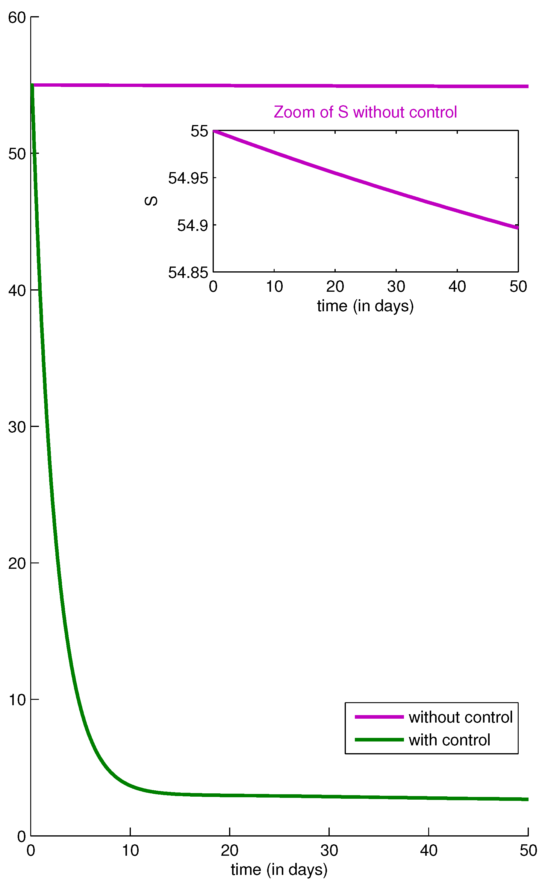
• S: the number of susceptible people to infection or who are not yet infected,
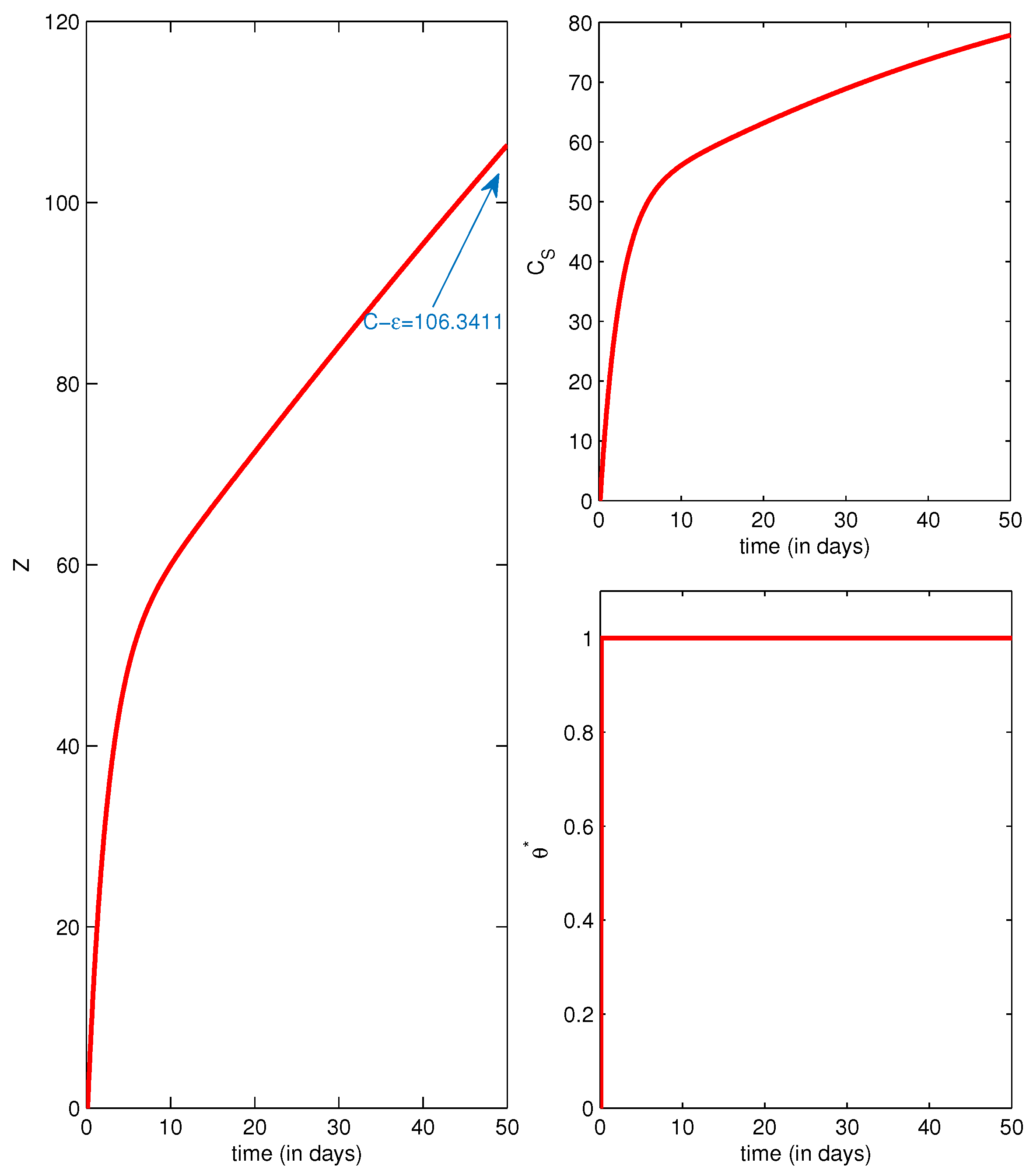
• $C_S$: the number of susceptible people who are temporarily controlled, so they cannot move to the removed class due to the limited effect of control. It can represent the compartment of vaccinated people in case a vaccination is not $100\%$ effective due to the difficulty of producing a perfect vaccine, the heterogeneity of the population or a vaccine not conferring a lifelong immunity [17,27],
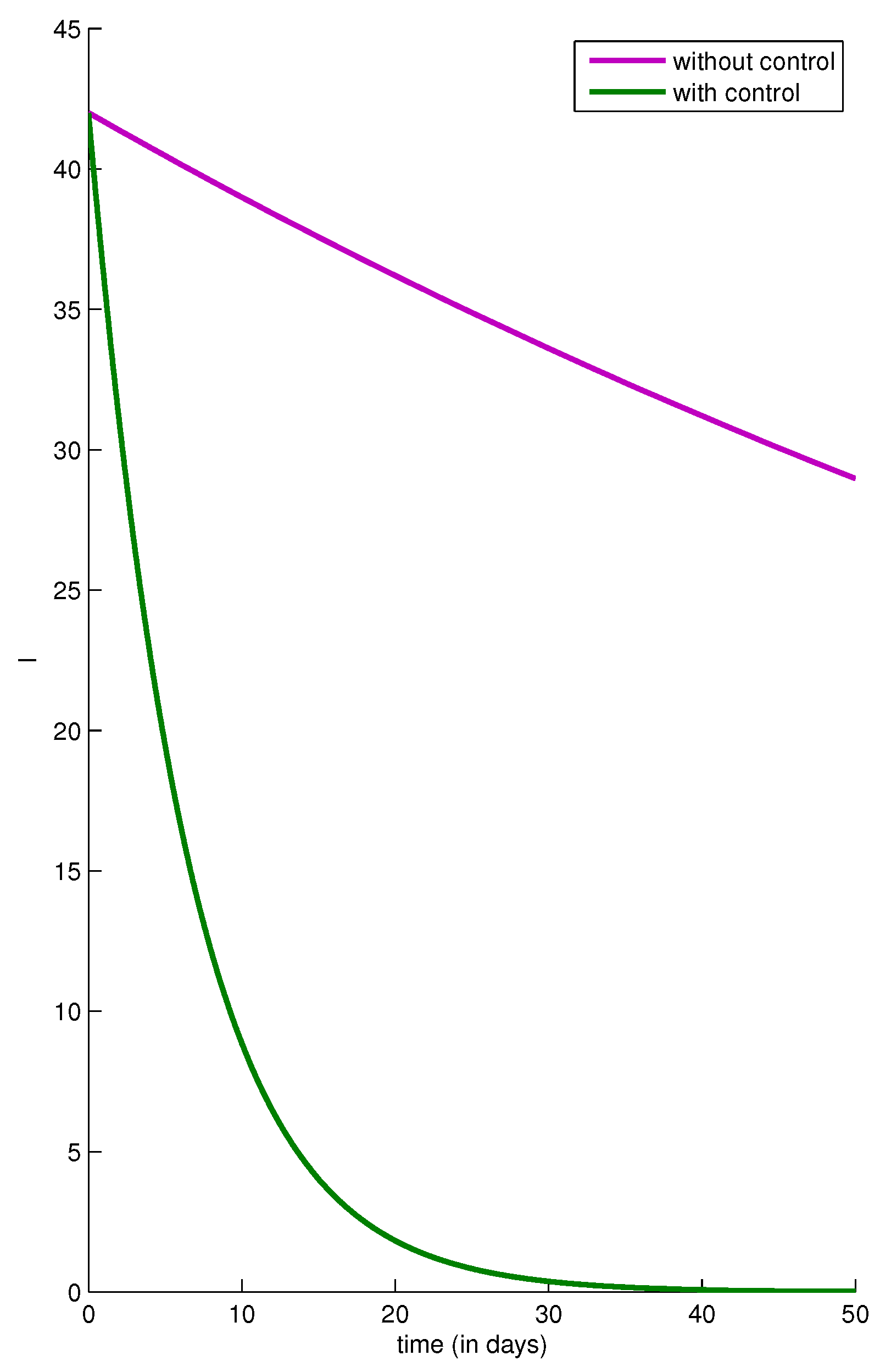
• I: the number of infected people who are capable of spreading the epidemic to those in the susceptible and temporarily controlled categories,
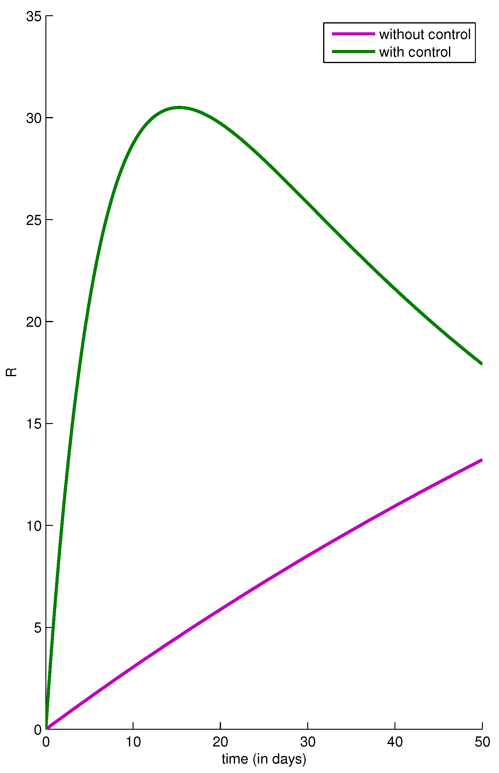
• R: the number of removed people from the epidemic, but can return to the susceptible class because of the short-term removal individuals’ immunity.

In our modeling approach, we aim to describe the dynamics of variables S, $C_S$, I and R at time i based on the following difference equations:

$$\left\{\begin{array}{ccc}{S}_{i+1}\hfill & =\hfill & S_i-\beta S_i{I}_i-a{\theta }_i{S}_i+{\Pi }_i-\mu S_i+\sigma R_i\hfill \\ C_{S_{i+1}}\hfill & =\hfill & C_{S_i}+a{\theta }_i{S}_i-b\beta C_{S_i}{I}_i-\mu C_{S_i}\hfill \\ I_{i+1}\hfill & =\hfill & I_i+\beta (S_i+b{C}_{S_i})I_i-\gamma I_i-\mu I_i\hfill \\ R_{i+1}\hfill & =\hfill & R_i+\gamma I_i-\mu R_i-\sigma R_i\hfill \end{array}\right.$$

(1)

with initial conditions $S_0>0$, $C_{S_0}\ge 0$, $I_0\ge 0$ and $R_0\ge 0$ and where ${\Pi }_i=\mu N_i$ with $N_i=S_i+C_{S_i}+I_i+R_i$, gives the newborn people, $a\theta$$(0\le a\le 1)$ is the recruitment rate of susceptibles to the controlled class with $\theta$ defining the control parameter as a constant between 0 and 1 (see such consideration in the case of vaccination in [27]) and “a” modeling the reduced chances of a susceptible individual to be controlled, $\beta =\frac{\delta }{N_i}$ with $\delta$ the infection transmission rate, $\mu$ the natural death rate, $b\theta$$(0\le b\le 1)$ the recruitment rate of controlled people to the infected class even in the presence of $\theta$ with “b” modeling the reduced chances of a temporarily controlled individual to be infected, $\gamma$ the recovery rate and $\sigma$ the losing removal individuals’ immunity rate. We note that the population size $N_i$ is constant at any time i because $N_{i+1}=S_{i+1}+C_{S_{i+1}}+I_{i+1}+R_{i+1}=N_i$. Hence, ${\Pi }_i=\Pi =constant$.

3. Methods

Now, we consider the mathematical model (1) with $\theta$ as a discrete control function.

Motivated by the desire to reduce the number of infected people as much as possible while minimizing the value of the control $\theta$ over N times, our objective is to seek an optimal control ${\theta }^{*}$ such that:

$${\displaystyle J\left({\theta }^{*}\right)=\underset{\theta \in \mathsf{\Theta }}{min}J\left(\theta \right)}$$

(2)

where J is the functional defined by:

$${\displaystyle J\left(\theta \right)=\sum _{i=0}^{N-1}\left({\displaystyle A{I}_i+\frac{B}{2}{\theta }_i^2}\right)+A{I}_N}$$

(3)

and where the control space $\mathsf{\Theta }$ is defined by the set:

$$\mathsf{\Theta }=\{\theta \in {\mathbb{R}}^N|{\theta }_{min}\le {\theta }_i\le {\theta }_{max},{\theta }_{max}\le 1{\theta }_{min}\ge 0,i=0,\dots ,N-1\left\}\right\}$$

A and B represent constant severity weights associated with functions I and $\theta$, respectively.

Managers of the anti-epidemic resources cannot well predict whether their control strategy will reach all the susceptible population over N times. To model the situation in which a restricted resource of control is available, we consider that the number of susceptible people we can control is equal to a constant $C>0$ for N days. Hence, we try to find ${\theta }^{*}$ under the definition of the following isoperimetric restriction:

$${\displaystyle C=\sum _{i=0}^{N-1}a{\theta }_i{S}_i}$$

(4)

In [25,26], the authors defined an isoperimetric constraint on the control variable only, to model the total tolerable dosage amount of a therapy along the treatment period. In their conferences talks [28,29], Kornienko et al. and de Pinho et al. introduced state constraints in an optimal control problem that is subject to an S-exposed-I-Rdifferential system to model the situation of the limited supply of vaccine based on the work in [24] and where the isoperimetric constraint is defined on the product of the control and state variables. Our study aims to highlight more the importance of such optimal control approaches by considering a discrete model rather than a continuous one. This would be interesting since data are often collected at discrete times, as noted in [30].

In our case, to take into account the constraint (4) for the resolution of the optimal control problem (2), we consider a new variable Z defined as:

$$Z_{i+1}=Z_i+a{\theta }_i{S}_i$$

(5)

with $Z_0=0$ and $Z_N=C$.

The discrete-time system of (1) becomes:

$$\begin{array}{c}\hfill \left\{\begin{array}{ccc}\hfill S_{i+1}& =& S_i+\Pi -\beta S_i{I}_i-a{\theta }_i{S}_i-\mu S_i+\sigma R_i\hfill \\ \hfill C_{S_{i+1}}& =& C_{S_i}+a{\theta }_i{S}_i-b\beta C_{S_i}{I}_i-\mu C_{S_i}\hfill \\ \hfill I_{i+1}& =& I_i+\beta (S_i+b{C}_{S_i})I_i-\gamma I_i-\mu I_i\hfill \\ \hfill R_{i+1}& =& R_i+\gamma I_i-\mu R_i-\sigma R_i\hfill \\ \hfill Z_{i+1}& =& Z_i+a{\theta }_i{S}_i\hfill \end{array}\right.\end{array}$$

(6)

In the following, we announce two theorems for proving the existence and the characterization of the sought optimal control ${\theta }^{*}$.

Theorem 1.

(Sufficient conditions) For the isoperimetric optimal control problem given by (2) along with the discrete state equations in (6), there exists a control ${\theta }^{*}\in \mathsf{\Theta }$ such that ${\displaystyle J\left({\theta }^{*}\right)=mi{n}_{\theta \in \mathsf{\Theta }}J\left(\theta \right)}$.

Proof. 

In order to prove the existence of a solution ${\theta }^{*}$ in $\mathsf{\Theta }$, we try to prove that ${min}_{\theta \in \mathsf{\Theta }}J\left(\theta \right)$ exists.

We have a finite number of time steps N and discrete state equations in System (6) with bounded coefficients $\gamma ,\mu ,b,\sigma ,\Pi ,a$ and $\beta$, then for all $\theta$ in the control set $\mathsf{\Theta }$, the N-component state variables:

$$\begin{array}{cc}\hfill S& =(S_0,S_1,\dots ,S_i,\dots ,S_{N-1}),\hfill \\ \hfill C_S& =(C_{S_0},C_{S_1},\dots ,C_{S_i},\dots ,C_{S_{N-1}}),\hfill \\ \hfill I& =(I_0,I_1,\dots ,I_i,\dots ,I_{N-1})\hfill \\ \hfill \mathrm{and}R& =(R_0,R_1,\dots ,R_i,\dots ,R_{N-1})\forall i=0,\dots ,N-1\hfill \end{array}$$

are uniformly bounded, which implies that $\forall \theta \in \mathsf{\Theta }$, $J\left(\theta \right)$ is uniformly bounded.

We can deduce then that $in{f}_{\theta \in \mathsf{\Theta }}J\left(\theta \right)$ is finite since $J\left(\theta \right)$ is bounded, and there exists a finite number j of uniformly bounded sequences ${\theta }^j\in \mathsf{\Theta }$ such that $li{m}_{j\to \infty }J\left({\theta }^j\right)=in{f}_{\theta \in \mathsf{\Theta }}J\left(\theta \right)$ and corresponding sequences of states $S^j,C_S^j,I^j$ and $R^j$.

Thus, there exists ${\theta }^{*}\in \mathsf{\Theta }$ and $S^{*},C_S^{*},I^{*},R^{*}\in {\mathbb{R}}^N$ such that on a subsequence,

$$\begin{array}{cc}\hfill {\theta }^j& \to {\theta }^{*},\hfill \\ \hfill S^j& \to S^{*},\hfill \\ \hfill C_S^j& \to C_S^{*},\hfill \\ \hfill I^j& \to I^{*}\hfill \\ \hfill \mathrm{and}{R}^j& \to R^{*}.\hfill \end{array}$$

Finally, due to the finite dimensional structure of the system (6) and the objective function $J\left(\theta \right)$, ${\theta }^{*}$ is an optimal control with corresponding states $S^{*},C_S^{*},I^{*}$ and $R^{*}$ [26]. Therefore, taking into account the structure of J being a convex function, $in{f}_{\theta \in \mathsf{\Theta }}J\left(\theta \right)$ is achieved. ☐

In order to derive the necessary conditions of optimality, we employ the discrete version of Pontryagin’s maximum principle stated in Theorem A1 in Appendix A.

Theorem 2.

(Necessary conditions) Given the optimal control${\theta }^{*}$and solutions $S^{*},C_S^{*},I^{*}$ and $R^{*}$, there exist ${\lambda }_{l,i},l=1,\dots ,5,i=0,\dots ,N$, the adjoint variables satisfying the following equations:

$$\begin{array}{ccc}\hfill \Delta {\lambda }_{1,i}& =& {\lambda }_{1,i+1}(-1+\beta I_i^{*}+\mu +a{\theta }_i^{*})-a{\lambda }_{2,i+1}{\theta }_i^{*}-\beta {\lambda }_{3,i+1}{I}_i^{*}-a{\theta }_i^{*}{\lambda }_{5,i+1}\hfill \end{array}$$

(7)

$$\begin{array}{ccc}\hfill \Delta {\lambda }_{2,i}& =& {\lambda }_{2,i+1}(-1+b\beta I_i^{*}+\mu )-b{\lambda }_{3,i+1}\beta I_i^{*}\hfill \end{array}$$

(8)

$$\begin{array}{ccc}\hfill \Delta {\lambda }_{3,i}& =& -A+{\lambda }_{1,i+1}\beta S_i^{*}+b{\lambda }_{2,i+1}\beta C_{S_i}^{*}-{\lambda }_{3,i+1}(-1+\beta (S_i^{*}+b{C}_{S_i}^{*})-\mu -\gamma )\hfill \\ & & -{\lambda }_{4,i+1}\gamma \hfill \end{array}$$

(9)

$$\begin{array}{ccc}\hfill \Delta {\lambda }_{4,i}& =& {\lambda }_{4,i+1}(\mu +\sigma -1)-\sigma {\lambda }_{1,i+1}\hfill \end{array}$$

(10)

$$\begin{array}{ccc}\hfill \Delta {\lambda }_{5,i}& =& -{\lambda }_{5,i+1}\hfill \end{array}$$

(11)

with $\Delta {\lambda }_{l,i}={\lambda }_{l,i+1}-{\lambda }_{l,i},l=1,\dots ,5,i=0,\dots ,N-1$ the difference operator and ${\lambda }_{1,N}={\lambda }_{2,N}={\lambda }_{4,N}=0$, ${\lambda }_{3,N}=A$ and ${\lambda }_{5,N}=constanttobedetermined$, as the transversality conditions associated with adjoint Equations (7)–(11).

In addition, the optimal control ${\theta }^{*}$ is characterized at each iteration i by:

$${\theta }_i^{*}=min\left(max\left({\displaystyle {\theta }_{min},\frac{a{S}_i^{*}\left({\lambda }_{1,i+1}-{\lambda }_{2,i+1}-{\lambda }_{5,i+1}\right)}{B}}\right),{\theta }_{max}\right)\forall i=0,\dots ,N-1$$

(12)

Proof. 

With the application of a discrete version of Pontryagin’s maximum principle in Appendix A and as done in [26,31,32], we can determine the discrete optimal control ${\theta }^{*}$ for the problem (6) and its associated trajectories $S^{*},C_S^{*},I^{*}$ and $R^{*}$.

We define a discrete Hamiltonian $H_i$ as a brief notation of the function H defined for $i=0,\dots ,N-1.$ as follows:

$$\begin{array}{c}{\displaystyle H(i,S_i,C_{S_i},I_i,R_i,{\lambda }_{1,i+1},{\lambda }_{2,i+1},{\lambda }_{3,i+1},{\lambda }_{4,i+1},{\lambda }_{5,i+1},{\theta }_i)}\hfill \\ {\displaystyle =A{I}_i+\frac{B}{2}{\theta }_i^2+{\lambda }_{1,i+1}{S}_{i+1}+{\lambda }_{2,i+1}{C}_{S_{i+1}}+{\lambda }_{3,i+1}{I}_{i+1}+{\lambda }_{4,i+1}{R}_{i+1}+{\lambda }_{5,i+1}{Z}_{i+1}}\hfill \end{array}$$

The discrete-time adjoint system is resolved using the following formulations:

$$\begin{array}{c}{\displaystyle \Delta {\lambda }_{1,i}=-\frac{\partial H_i}{\partial S_i},\Delta {\lambda }_{2,i}=-\frac{\partial H_i}{\partial C_{S_i}},\Delta {\lambda }_{3,i}=-\frac{\partial H_i}{\partial I_i},\Delta {\lambda }_{4,i}=-\frac{\partial H_i}{\partial R_i}}\hfill \\ {\displaystyle \mathrm{and}\Delta {\lambda }_{5,i}=-\frac{\partial H_i}{\partial Z_i}}\hfill \end{array}$$

that we associate with the following transversality conditions:

$$\begin{array}{c}\hfill {\displaystyle {\lambda }_{1,N}=\frac{\partial {\varphi }_N}{\partial S_N},{\lambda }_{2,N}=\frac{\partial {\varphi }_N}{\partial C_{S_N}},{\lambda }_{3,N}=\frac{\partial {\varphi }_N}{\partial I_N},{\lambda }_{4,N}=\frac{\partial {\varphi }_N}{\partial R_N}}\end{array}$$

with ${\varphi }_N$ representing the payoff term function in (3), namely $A{I}_N$.

Then, we obtain the following discrete-time adjoint system:

$$\left\{\begin{array}{ccc}\hfill \Delta {\lambda }_{1,i}& =& {\lambda }_{1,i+1}(-1+\beta I_i+\mu +a{\theta }_i)-a{\lambda }_{2,i+1}{\theta }_i-\beta {\lambda }_{3,i+1}{I}_i-a{\theta }_i{\lambda }_{5,i+1}\hfill \\ \hfill \Delta {\lambda }_{2,i}& =& {\lambda }_{2,i+1}(-1+b\beta I_i+\mu )-b{\lambda }_{3,i+1}\beta I_i\hfill \\ \hfill \Delta {\lambda }_{3,i}& =& -A+{\lambda }_{1,i+1}\beta S_i+b{\lambda }_{2,i+1}\beta C_{S_i}-{\lambda }_{3,i+1}(-1+\beta (S_i+b{C}_{S_i})-\mu -\gamma )-{\lambda }_{4,i+1}\gamma \hfill \\ \hfill \Delta {\lambda }_{4,i}& =& {\lambda }_{4,i+1}(\mu +\sigma -1)-\sigma {\lambda }_{1,i+1}\hfill \\ \hfill \Delta {\lambda }_{5,i}& =& -{\lambda }_{5,i+1}\hfill \end{array}\right.$$

with the transversality conditions ${\lambda }_{1,N}=0,{\lambda }_{2,N}=0,{\lambda }_{4,N}=0,{\lambda }_{3,N}=A$ and ${\lambda }_{5,N}$ is unknown.

In order to find the transversality condition ${\lambda }_{5,N}=constant$, we use the secant-method as the appropriate numerical technique for finding the zero of the function ${\lambda }_{5,N}\to V\left({\lambda }_{5,N}\right)={\tilde{Z}}_N-Z_N$ where ${\tilde{Z}}_N$ is the value of Z at final iteration N for various values of ${\lambda }_{5,N}$ and $Z_N$ is the value fixed by C [25,33].

Since ${\theta }_i$ is a bounded control, we can then define a Lagrangian L as follows:

$$\begin{array}{c}L((i,S_i,C_{S_i},I_i,R_i,{\lambda }_{1,i+1},{\lambda }_{2,i+1},{\lambda }_{3,i+1},{\lambda }_{4,i+1},{\lambda }_{5,i+1},{\theta }_i,{\omega }_{1,i},{\omega }_{2,i})\hfill \\ =H_i+{\omega }_{1,i}({\theta }_{max}-{\theta }_i)+{\omega }_{2,i}({\theta }_i-{\theta }_{min})\hfill \end{array}$$

where ${\omega }_{1,i},{\omega }_{2,i}\ge 0\forall i$ verifying at ${\theta }_i={\theta }_i^{*}$, the two conditions ${\omega }_{1,i}({\theta }_{max}-{\theta }_i^{*})=0$ and ${\omega }_{2,i}({\theta }_i^{*}-{\theta }_{min})=0$.

Let $L_i$ be the brief notation of L and $L_i^{*}$ be the brief notation of L at $S^{*},C_S^{*},I^{*},R^{*}$ and ${\theta }^{*}$. The condition of minimization is defined as:

$$\begin{array}{c}\hfill {\displaystyle L_i^{*}=\underset{{\theta }_i\in \mathsf{\Theta }}{min}{L}_i{(}^{**}).}\end{array}$$

In order to find the solution ${\theta }_i^{*}$ of ${(}^{**})$, we differentiate the Lagrangian $L_i$ with respect to ${\theta }_i$ on the set $\mathsf{\Theta }$ to obtain the optimality equation:

$$\begin{array}{c}\hfill {\displaystyle \frac{\partial L_i}{\partial {\theta }_i}=B{\theta }_i+a{S}_i({\lambda }_{2,i+1}-{\lambda }_{1,i+1})+a{S}_i{\lambda }_{5,i+1}-{\omega }_{1,i}+{\omega }_{2,i}=0\mathrm{at}{\theta }_i^{*}.}\end{array}$$

Furthermore, we find

$${\displaystyle {\theta }_i^{*}=\frac{a{S}_i^{*}\left({\lambda }_{1,i+1}-{\lambda }_{2,i+1}-{\lambda }_{5,i+1}\right)-{\omega }_{2,i}+{\omega }_{1,i}}{B}.}$$

If:

$$\begin{array}{c}\hfill {\theta }_{min}<{\theta }_i^{*}<{\theta }_{max},\end{array}$$

then:

$$\begin{array}{c}\hfill {\omega }_{1,i}={\omega }_{2,i}=0,\end{array}$$

therefore:

$$\begin{array}{c}\hfill {\displaystyle {\theta }_i^{*}=\frac{a{S}_i^{*}\left({\lambda }_{1,i+1}-{\lambda }_{2,i+1}-{\lambda }_{5,i+1}\right)}{B}.}\end{array}$$

If:

$$\begin{array}{c}\hfill {\theta }_i^{*}={\theta }_{min},\end{array}$$

then:

$$\begin{array}{c}\hfill {\omega }_{1,i}=0,\end{array}$$

therefore:

$$\begin{array}{c}\hfill {\displaystyle {\theta }_{min}=\frac{a{S}_i^{*}\left({\lambda }_{1,i+1}-{\lambda }_{2,i+1}-{\lambda }_{5,i+1}\right)-{\omega }_{2,i}}{B},}\end{array}$$

implying that:

$$\begin{array}{c}\hfill {\omega }_{2,i}=a\left(S_i^{*}({\lambda }_{1,i+1}-{\lambda }_{2,i+1})-S_i^{*}{\lambda }_{5,i+1}\right)-B{\theta }_{min}.\end{array}$$

Knowing that ${\omega }_{2,i}\ge 0$ and $B>0,$ we obtain ${\displaystyle {\theta }_i^{*}\le \frac{a{S}_i^{*}\left({\lambda }_{1,i+1}-{\lambda }_{2,i+1}-{\lambda }_{5,i+1}\right)}{B}}$.

If:

$$\begin{array}{c}\hfill {\theta }_i^{*}={\theta }_{max},\end{array}$$

then:

$$\begin{array}{c}\hfill {\omega }_{2,i}=0,\end{array}$$

thus:

$$\begin{array}{c}\hfill {\displaystyle {\theta }_{max}=\frac{a{S}_i^{*}\left({\lambda }_{1,i+1}-{\lambda }_{2,i+1}-{\lambda }_{5,i+1}\right)+{\omega }_{1,i}}{B},}\end{array}$$

implying that ${\omega }_{1,k}=B{\theta }_{max}-a\left(S_i^{*}({\lambda }_{1,i+1}-{\lambda }_{2,i+1})-S_i^{*}{\lambda }_{5,i+1}\right)$.

Knowing that ${\omega }_{1,i}\ge 0$ and $B>0,$ we obtain ${\displaystyle {\theta }_i^{*}\ge \frac{a{S}_i^{*}\left({\lambda }_{1,i+1}-{\lambda }_{2,i+1}-{\lambda }_{5,i+1}\right)}{B}}$.

Using these standard optimality arguments, we characterize the control $u_k^{*}$ by:

$$\begin{array}{c}\hfill {\theta }_i^{*}=\left\{\begin{array}{c}\frac{a{S}_i^{*}\left({\lambda }_{1,i+1}-{\lambda }_{2,i+1}-{\lambda }_{5,i+1}\right)}{B}\mathrm{if}{\theta }_{min}<\frac{a{S}_i^{*}\left({\lambda }_{1,i+1}-{\lambda }_{2,i+1}-{\lambda }_{5,i+1}\right)}{B}<{\theta }_{max}\\ {\theta }_{min}\mathrm{if}\frac{a{S}_i^{*}\left({\lambda }_{1,i+1}-{\lambda }_{2,i+1}-{\lambda }_{5,i+1}\right)}{B}\le {\theta }_{min}\\ {\theta }_{max}\mathrm{if}\frac{a{S}_i^{*}\left({\lambda }_{1,i+1}-{\lambda }_{2,i+1}-{\lambda }_{5,i+1}\right)}{B}\ge {\theta }_{max}\end{array}\right.\end{array}$$

or by a more reduced form, we can write

$${\theta }_i^{*}=min\left(max\left({\displaystyle {\theta }_{min},\frac{a{S}_i^{*}\left({\lambda }_{1,i+1}-{\lambda }_{2,i+1}-{\lambda }_{5,i+1}\right)}{B}}\right),{\theta }_{max}\right)$$

 ☐

4. Numerical Results and Discussion

In this section, we resolve the discrete two-point value problem defined by System (6) with initial conditions along with Equations (7)–(11) with final conditions, using a discrete version of the forward-backward sweep method (FBSM) [26,33] with the incorporation of a discrete progressive iterative scheme to stock at each iteration i, the values of the state variables corresponding to the forward discrete-time system (6), to use them in a second discrete regressive iterative scheme incorporated for stocking at each time i, the values of the adjoint state variables corresponding to the backward discrete-time adjoint system (7)–(11). In fact, at each time i, the values stocked of both state and adjoint state variables were utilized in the characterization of the optimal control ${\theta }^{*}$. In brief, our algorithm is defined by the following four steps of numerical calculus (Algorithm 1).

Algorithm 1: Resolution steps of the discrete two-point boundary value optimal control problem (6)–(11).

Step 0:  Guess an initial estimation of θ. Step 1:  Use the initial condition $S\left(0\right)$, $C_S\left(0\right)$, $I\left(0\right)$, $R\left(0\right)$ and $Z\left(0\right)$ and the stocked values by θ.  Find the optimal states $S^{*}$, $C_S^{*}$, $I^{*}$, $R^{*}$ and $Z^{*}$, which iterate forward in the discrete two-point boundary value problem (6). Step 2:  Use the stocked values by θ and the transversality conditions ${\lambda }_{l,N+1}$ for $l=1,2,3,4$ while searching the constant ${\lambda }_{5,N+1}$ using the secant-method. More precisely, the secant method is used to obtain the zero of the function ${\lambda }_{5,N}\to V\left({\lambda }_{5,N}\right)={\tilde{Z}}_N-Z_N$ where ${\tilde{Z}}_N$ is the value of Z at final iteration N for various values of ${\lambda }_{5,N}$, and $Z_N$ is the value fixed by C. In addition, due its structure in (4), we choose the constant C in a way that it cannot exceed an upper bound $N_0\times N$ where $N_0$ is the initial population size and N is the number of iterations.  Find the adjoint variables ${\lambda }_l$ for $l=1,2,3,4,5$, which iterate backward in the discrete two-point boundary value problem (6). Step 3:  Update the control utilizing new S, $C_S$, I, R, Z and ${\lambda }_l$ for $l=1,2,3,4,5$ in the characterization of ${\theta }^{*}$ as presented in (12). Step 4:  Test the convergence. If the values of the sought variables in this iteration and the final iteration are sufficiently small, check out the recent values as solutions. If the values are not small, go back to Step 1.

Figure 1 depicts the behavior of the number of susceptible people in the absence and presence of the control, and we can see that the number of susceptible people had decreased from its initial condition once the control had been introduced, while there was no significant decrease of the S function compared to the case when there was yet no control. With these parameters used, it reached only three people because of the maximal value of one taken by the optimal control ${\theta }^{*}$ in almost alltimes of the control strategy, as seen in the last figure.

In Figure 2, we can well understand the increase of the number of the removed people because of a natural recovery, but it cannot represent a significant recovery because it has not reached even 14 people, and this means that only a very small number of people have been removed based on the initial condition $I\left(0\right)$ considered. In the presence of the control, the R function increased towards a much higher number of removed people and showed it can even reach more than 31 individuals recovered from the disease in the first 17 days; this number decreased thereafter because of the results in the next figure, which will show that infection will disappear as we move forward in time.

In Figure 3, the simulation shows that the number of infected people could decrease only because of a natural recovery or death, while the infection was still serious and remained present in more than 28 individuals. After the introduction of the control, the I function started to decrease once the anti-epidemic was followed, and it tended to zero values after 37 days; this means most people would recover from the disease at the end of the control strategy.

As regards Figure 4, we sought to verify the condition $C=110$, which meets the value $2\times S_0$, and we presented associated simulations of the number of controlled people, which increased to 53 individuals once the optimal control had been introduced and increased thereafter, again showing that it could even exceed that number, approximately towards 80 people when we go forward towards the end. In the same figure, we show the values of the optimal control ${\theta }^{*}$, which take the value of one as the maximal peak for almost alldays, and we can also see that the imposed isoperimetric constant has been verified in the final instant with some error $ϵ=3.6589$. In fact, it is not evident that it reached any imposed value while verifying convergence tests of both methods used. Sometimes, the program did not stop iterating or could not show the plot because of a NANvalue, and then, the only solution was to fix the number of iterations of the secant method in which the imposed initial guess of C was approximately reached.

In Figure 5, we exhibit the value of the sought constant missing transversality condition ${\lambda }_{5,N}$, which will be essential to verify the necessary conditions announced in Theorem 2. As we can observe from this figure, the value obtained equals $-1.3830\times {10}^8$.

Figure 6 presents a numerical simulation of the Z function when we did not seek the verification of the condition $Z_N=C$, and we let $Z_N$ free, so we could prove that our algorithm in the case of the isoperimetric constraint helped to approximate $Z_N$ to C or even verify the equality between them, far from the value that could reach $Z_N$ when it was free; as we can see from the mentioned figure, $Z_N=105.5729$, which led to an important error of about 4.4271 from C that was sought in Figure 4.

5. Conclusions

In this paper, an optimal control approach with an isoperimetric constraint has been applied to a discrete-time SIRS model, which was in the form of a four-compartmental epidemic model where it was supposed that the controlled population did not reach the removed class due to the temporary effect of the control. The isoperimetric restriction, which has been proposed to define the number of susceptible people who receive the control along the anti-epidemic measures period, allowed us to find the optimal control needed to fight against a disease when there were limited resources.

References

1. Kermack, W.O.; McKendrick, A.G. A Contribution to the Mathematical Theory of Epidemics. Proc. R. Soc. A 1927, 115, 700–721. [Google Scholar] [CrossRef] [Green Version]
2. Acedo, L.; González-Parra, G.; Arenas, A.J. An exact global solution for the classical SIRS epidemic model. Nonlinear Anal. Real World Appl. 2010, 11, 1819–1825. [Google Scholar] [CrossRef]
3. Alexander, M.E.; Moghadas, S.M. Bifurcation analysis of an SIRS epidemic model with generalized incidence. SIAM J. Appl. Math. 2005, 65, 1794–1816. [Google Scholar] [CrossRef]
4. Hu, Z.; Bi, P.; Ma, W.; Ruan, S. Bifurcations of an SIRS epidemic model with nonlinear incidence rate. Discret. Contin. Dyn. Syst. Ser. B 2011, 15, 93–112. [Google Scholar]
5. Teng, Z.; Liu, Y.; Zhang, L. Persistence and extinction of disease in non-autonomous SIRS epidemic models with disease-induced mortality. Nonlinear Anal. Theory Methods Appl. 2008, 69, 2599–2614. [Google Scholar] [CrossRef]
6. Xamxinur, A.; Teng, Z. On the persistence and extinction for a non–autonomous SIRS epidemic model. J. Biomath. 2006, 21, 167–176. [Google Scholar]
7. Jin, Y.; Wang, W.; Xiao, S. An SIRS model with a nonlinear incidence rate. Chaos Solitons Fractals 2007, 34, 1482–1497. [Google Scholar]
8. Liu, J.; Zhou, Y. Global stability of an SIRS epidemic model with transport-related infection. Chaos Solitons Fractals 2009, 40, 145–158. [Google Scholar]
9. Chen, J. An SIRS epidemic model. Appl. Math. J. Chin. Univ. 2004, 19, 101–108. [Google Scholar]
10. Hu, Z.; Teng, Z.; Jiang, H. Stability analysis in a class of discrete SIRS epidemic models. Nonlinear Anal. Real World Appl. 2012, 13, 2017–2033. [Google Scholar] [CrossRef]
11. Mukhopadhyay, B.B.; Tapaswi, P.K. An SIRS epidemic model of Japanese encephalitis. Int. J. Math. Math. Sci. 1994, 17, 347–355. [Google Scholar] [CrossRef]
12. Abouelkheir, I.; El Kihal, F.; Rachik, M.; Zakary, O.; Elmouki, I. A multi-regions SIRS discrete epidemic model with a travel-blocking vicinity optimal control approach on cells. Br. J. Math. Comput. Sci. 2017, 20, 1–16. [Google Scholar] [CrossRef] [PubMed]
13. Zakary, O.; Rachik, M.; Elmouki, I. On the impact of awareness programs in HIV/AIDS prevention: An SIR model with optimal control. Int. J. Comput. Appl. 2016, 133. [Google Scholar] [CrossRef]
14. Zakary, O.; Larrache, A.; Rachik, M.; Elmouki, I. Effect of awareness programs and travel-blocking operations in the control of HIV/AIDS outbreaks: A multi-domains SIR model. Adv. Differ. Equ. 2016, 2016, 169. [Google Scholar] [CrossRef]
15. Shim, E. A note on epidemic models with infective immigrants and vaccination. Math. Biosci. Eng. 2006, 3, 557. [Google Scholar] [CrossRef] [PubMed]
16. Roy, P.K.; Saha, S.; Al Basir, F. Effect of awareness programs in controlling the disease HIV/AIDS: An optimal control theoretic approach. Adv. Differ. Equ. 2015, 2015, 217. [Google Scholar] [CrossRef]
17. Rodrigues, H.S.; Monteiro, M.T.T.; Torres, D.F. Vaccination models and optimal control strategies to dengue. Math. Biosci. 2014, 247, 1–12. [Google Scholar] [CrossRef] [PubMed] [Green Version]
18. Kumar, A.; Srivastava, P.K. Vaccination and treatment as control interventions in an infectious disease model with their cost optimization. Commun. Nonlinear Sci. Numer. Simul. 2017, 44, 334–343. [Google Scholar] [CrossRef]
19. Liu, X.; Takeuchi, Y.; Iwami, S. SVIR epidemic models with vaccination strategies. J. Theor. Biol. 2008, 253, 1–11. [Google Scholar] [CrossRef] [PubMed]
20. Nainggolan, J.; Supian, S.; Supriatna, A.K.; Anggriani, N. Mathematical model of tuberculosis transmission with reccurent infection and vaccination. In Journal of Physics: Conference Series; IOP Publishing: Bristol, UK, 2013; Volume 423, No. 1; p. 012059. [Google Scholar]
21. Zhou, L.; Fan, M. Dynamics of an SIR epidemic model with limited medical resources revisited. Nonlinear Anal. Real World Appl. 2012, 13, 312–324. [Google Scholar] [CrossRef]
22. Abdelrazec, A.; Bélair, J.; Shan, C.; Zhu, H. Modeling the spread and control of dengue with limited public health resources. Math. Biosci. 2016, 271, 136–145. [Google Scholar] [CrossRef] [PubMed]
23. Yu, T.; Cao, D.; Liu, S. Epidemic model with group mixing: Stability and optimal control based on limited vaccination resources. Commun. Nonlinear Sci. Numer. Simul. 2018, 61, 54–70. [Google Scholar] [CrossRef]
24. Neilan, R.M.; Lenhart, S. An Introduction to Optimal Control with an Application in Disease Modeling. In Modeling Paradigms and Analysis of Disease Trasmission Models; American Mathematical Society: Providence, RI, USA, 2010; pp. 67–82. [Google Scholar]
25. Elmouki, I.; Saadi, S. BCG immunotherapy optimization on an isoperimetric optimal control problem for the treatment of superficial bladder cancer. Int. J. Dyn. Control 2016, 4, 339–345. [Google Scholar] [CrossRef]
26. Alkama, M.; Rachik, M.; Elmouki, I. A discrete isoperimetric optimal control approach for BCG immunotherapy in superficial bladder cancer: Discussions on results of different optimal doses. Int. J. Appl. Comput. Math. 2017, 3, 1–18. [Google Scholar] [CrossRef]
27. Sharomi, O.; Malik, T. Optimal control in epidemiology. Ann. Oper. Res. 2017, 251, 55–71. [Google Scholar] [CrossRef]
28. Kornienko, I.; Paiva, L.T.; De Pinho, M.D.R. Introducing state constraints in optimal control for health problems. Procedia Technol. 2014, 17, 415–422. [Google Scholar] [CrossRef]
29. De Pinho, M.D.R.; Kornienko, I.; Maurer, H. Optimal control of a SEIR model with mixed constraints and L 1 cost. In Proceedings of the 11th Portuguese Conference on Automatic Control, CONTROLO’2014, Porto, Portugal, 21–23 July 2014; Springer: Cham, Switzerland, 2015; pp. 135–145. [Google Scholar]
30. Zakary, O.; Rachik, M.; Elmouki, I. On the analysis of a multi-regions discrete SIR epidemic model: An optimal control approach. Int. J. Dyn. Control 2017, 5, 917–930. [Google Scholar] [CrossRef]
31. Zakary, O.; Rachik, M.; Elmouki, I.; Lazaiz, S. A multi-regions discrete-time epidemic model with a travel-blocking vicinity optimal control approach on patches. Adv. Differ. Equ. 2017, 2017, 120. [Google Scholar] [CrossRef]
32. Zakary, O.; Rachik, M.; Elmouki, I. A new epidemic modeling approach: Multi-regions discrete-time model with travel-blocking vicinity optimal control strategy. Infect. Dis. Model. 2017, 2, 304–322. [Google Scholar] [CrossRef] [PubMed]
33. Lenhart, S.; Workman, J.T. Optimal Control Applied to Biological Models; CRC Press: Boca Raton, FL, USA, 2007. [Google Scholar]
34. Sethi, S.P.; Thompson, G.L. What Is Optimal Control Theory? Springer: New York, NY, USA, 2000; pp. 1–22. [Google Scholar]
Figure 1. Number of susceptible people in the absence and presence of the control in the two cases θ = 0 and θ 0 . Parameter values: Π = μ N 0 , a = 0.5 , b = 0.1 , β = 10 5 , μ = 0.00045 , γ = 0.75 × 10 2 , σ = 5 × 10 4 . Initial conditions: S ( 0 ) = 55 , C S ( 0 ) = 0 , I ( 0 ) = 42 , R ( 0 ) = 0 . Severity weight constants: A = 1 and B = 4 × 10 5 .
Mca 23 00052 g001
Figure 2. Number of removed people in the absence and presence of the control in the two cases θ = 0 and θ 0 , with the same parameter values, initial conditions and severity weights as in Figure 1.
Mca 23 00052 g002
Figure 3. Number of infected people in the absence and presence of the control in the two cases θ = 0 and θ 0 , with the same parameter values, initial conditions and severity weights as in Figure 1.
Mca 23 00052 g003
Figure 4. Number of controlled people, the optimal control θ * and the variable Z with an imposed constant C = 110 , with the same parameter values, initial conditions and severity weights as in Figure 1.
Mca 23 00052 g004
Figure 5. Value of the sought transversality condition λ 5 , N .
Mca 23 00052 g005
Figure 6. Z function when Z N is free and not forced to equal C.
Mca 23 00052 g006