Heavy Ball Restarted CMRH Methods for Linear Systems

Abstract

The restarted CMRH method (changing minimal residual method based on the Hessenberg process) using fewer operations and storage is an alternative method to the restarted generalized minimal residual method (GMRES) method for linear systems. However, the traditional restarted CMRH method, which completely ignores the history information in the previous cycles, presents a slow speed of convergence. In this paper, we propose a heavy ball restarted CMRH method to remedy the slow convergence by bringing the previous approximation into the current search subspace. Numerical examples illustrate the effectiveness of the heavy ball restarted CMRH method.

1. Introduction

In this paper, we are concerned with the CMRH method (changing minimal residual method based on the Hessenberg process) introduced in [1,2] for the solution of $n\times n$ linear system $Ax=b$. Given an initial approximation $x_0$, and letting the initial residual $r_0=b-A{x}_0$, the CMRH method is a Krylov subspace method based on the m-dimensional Krylov subspace

$${\mathcal{K}}_m(A,r_0)=span\{r_0,A{r}_0,\dots ,A^{m-1}{r}_0\}.$$

(1)

It can also be considered as an alternative method of the generalized minimal residual method (GMRES) [3]. Nevertheless, they generate different basis vectors in different ways. The GMRES method uses the Arnoldi process to construct an orthonormal basis matrix of the m-dimensional Krylov subspace (1), while the CMRH method is based on the Hessenberg process [4], which requires half as much arithmetic work and less storage than the GMRES method. The corresponding convergence analysis of the CMRH method and its relation to the GMRES method can be found in [5,6]. There are a great deal of past and recent works and interests in developing the Hessenberg process and CMRH method for linear systems [7,8,9,10,11,12,13]. Specifically, in [7,8], Duminil presents an implementation for parallel architectures and an implementation of the left preconditioned CMRH method. A polynomial preconditioner and flexible right preconditioner for CMRH methods are considered in [9] and [10], respectively. In [12,13], the variants of the Hessenberg and CMRH methods are introduced for solving multi-shifted non-Hermitian linear systems.

Although the CMRH method is less expensive and needs less storage than the GMRES method per iteration, for large-scale linear systems, it is still very expensive for large m. In addition, the number of vectors requiring storage also increases as m increases. Hence, the method must be restarted. The restarted CMRH method denoted by CMRH(m) [1] is naturally developed to alleviate the possibly heavy memory burden and arithmetic operations cost. However, the price to pay for the restart is usually slower speed of the convergence. In the restarted GMRES methods, in order to overcome the slow convergence, there are many other effectiveness restarting technologies [14,15,16,17] which are designed to improve the simplest version of the restarted GMRES methods. Nevertheless, the research on the restarted CMRH method is rather scarce. One of the reasons is because the basis vectors generated by the Hessenberg process are not orthonormal. This leads to the CMRH residual vector being not orthogonal to the subspace ${\mathcal{K}}_m(A,r_0)$ or $A\times {\mathcal{K}}_m(A,r_0)$. Thus, the whole augmented subspace containing the smaller Krylov subspace with Ritz vectors or harmonic Ritz vectors is not still a Krylov subspace. (See the subspace (2.4) of [17] for more details on this augmented subspace.) This means that the restarting strategy by including eigenvectors associated with the few smallest eigenvalues into the Krylov subspace [15,16,17] is not available in the restarted CMRH methods. In this paper, inspired by the locally optimal conjugate gradient (LOCG) methods for the eigenvalue problem [18,19,20,21,22,23] and the locally optimal and heavy ball GMRES methods for linear systems [14], we propose a heavy ball restarted CMRH method to keep the benefit and remedy the lost convergence speed of the traditional restarted CMRH method. For traditional restarted CMRH method (i.e., CMRH(m)), each CMRH cycle builds a Krylov subspace for computing the approximate solution of the cycle, which is used as the initial guess for the next cycle. As soon as the approximation is computed, the built Krylov subspace is thrown away. Nevertheless, in the heavy ball restarted CMRH method proposed in this paper, for salvaging the loss of the previous search space, we take the previous approximation into the current search to bring sufficient history information of the previous Krylov subspace.

The rest of this paper is organized as follows. In Section 2, we briefly review the Hessenberg process and the restarted CMRH method, then introduce the algorithmic framework and implementation details of the heavy ball restarted CMRH method. Numerical examples are given in Section 3 to show the convergence behavior of the improved method. Finally, we give our concluding remarks in Section 4.

Notation. Throughout this paper, ${\mathbb{R}}^{n\times m}$ is the set of all $n\times m$ real matrices, ${\mathbb{R}}^n={\mathbb{R}}^{n\times 1}$ and $\mathbb{R}={\mathbb{R}}^1$. $I_n$ is the $n\times n$ identity matrix, and $e_j^{(n)}$ is its jth column. The superscript “.${}^T$” takes the transpose only of a matrix or vector. For a vector u and a matrix A, $u(j)$ is u’s jth entry, $u(i:j)$ is the vector of components $u(i),\dots ,u(j)$, and $A(i,j)$ is A’s $(i,j)$th entry. Notations ${\parallel ·\parallel }_1$, ${\parallel ·\parallel }_2$ and ${\parallel ·\parallel }_{\infty }$ are the 1-norm, 2-norm, and ∞-norm of a vector or matrix, respectively.

2. The Heavy Ball Restarted CMRH Method

2.1. The Hessenberg Process with Pivoting

The CMRH method [1] for the linear systems $Ax=b$ is based on the Hessenberg process with pivoting as given in Algorithm 1 to construct a basis of the Krylov subspace ${\mathcal{K}}_m(A,r_0)$. Given an initial guess $x_0\in {\mathbb{R}}^n$, the recursively computed basis matrix $L_m=[{\ell }_1,\dots ,{\ell }_m]\in {\mathbb{R}}^{n\times m}$ and the upper Hessenberg matrix $H_m\in {\mathbb{R}}^{m\times m}$ by Algorithm 1 satisfy

$$A{L}_m=L_{m+1}{\stackrel{̲}{H}}_m=L_m{H}_m+h_{m+1,m}{\ell }_{m+1}{(e_m^{(m)})}^T,$$

where ${\stackrel{̲}{H}}_m=\left[\begin{array}{c}{H}_m\\ h_{m+1,m}{(e_m^{(m)})}^T\end{array}\right]$ and $P{L}_m$ is a unit lower trapezoidal matrix with $P^T=[e_{p(1)}^{(n)},\dots ,e_{p(n)}^{(n)}]$. In particular, the initial residual vector $r_0={\beta }_0\times {\ell }_1={\beta }_0\times L_{m+1}{e}_1^{(m+1)}$, where ${\beta }_0=r_0(i_0)$ as defined in Line 2 of Algorithm 1.

Algorithm 1 Hessenberg process with pivoting

1: Choose an initial guess $x_0\in {\mathbb{R}}^n$ and an integer $m\ge 1$. 2: Let $r_0=b-A{x}_0$. Set $p=[1,\dots ,n]$ and determine $i_0$ such that $|r_0(i_0)|=\parallel r_0{\parallel }_{\infty }$, ${\beta }_0=r_0(i_0)$, ${\ell }_1=r_0/{\beta }_0$, and $p(1)\leftrightarrow p(i_0)$ where “↔” means swap contents. 3: for $j=1,2,\dots ,m$ do 4:  $u=A{\ell }_j$. 5:  for $i=1,2,\dots ,j$ do 6:   $h_{i,j}=u(p(i))$, $u=u-h_{i,j}{\ell }_i$. 7:  end for 8:  if ($j<n$ and $u\ne 0$) then 9:   Determine $j_0\in \{j+1,\dots ,n\}$ such that $|u(p(j_0))|=\parallel u\left(p(j+1:n)\right){\parallel }_{\infty }$. 10:   $h_{j+1,j}=u(p(j_0))$, ${\ell }_{j+1}=u/h_{j+1,j}$ and $p(j+1)\leftrightarrow p(j_0)$. 11:  else 12:   $h_{j+1,j}=0$. Stop. 13:  end if 14: end for

The CMRH approximate solution $x_m$ is obtained as $x_0+z_m$, where $z_m$ solves

$$\underset{z\in {\mathcal{K}}_m(A,r_0)}{min}{\parallel L_{m+1}^{†}\left(b-A(x_0+z)\right)\parallel }_2.$$

Here, $L_{m+1}^{†}$ is the pseudo-inverse of $L_{m+1}$. In fact, any left inverse of $L_{m+1}$ will work, but we use the pseudo-inverse here for simplicity. We can state equivalently that $x_m=x_0+L_m{y}_m$, where $y_m=arg\underset{y\in {\mathbb{R}}^m}{min}{\parallel {\beta }_0{e}_1^{(m+1)}-{\stackrel{̲}{H}}_{m}y\parallel }_2$. Like the quasi-minimal residual (QMR)  method [24], the CMRH method is a quasi-residual minimization method.

2.2. The Heavy Ball Restarted CMRH (HBCMRH) Method

To alleviate a heavy demand on memory, the restarted CMRH method (or CMRH(m) for short) is implemented by fixing m and repeating the m-step CMRH method with the current initial guess $x_0^{(k)}$ being the previous approximation solution $x_m^{(k-1)}$, where the kth and $(k-1)$th CMRH cycles are indexed by the superscript “(k)” and “($k-1$)”, respectively. By limiting the number m in the Hessenberg process, although CMRH(m) successfully remedies possibly heavy memory burden and computational cost, at the same time it sometimes converges slowly. One of the reasons is that all the Krylov subspaces built in the previous cycles are completely ignored. Motivated by the locally optimal and heavy ball CMRES method [14] which is proposed by including the approximation before the last to bring in more information in the previous cycles, we naturally develop a heavy ball restarted CMRH method denoted by HBCMRH(m) to make up the loss of previous search spaces. For each cycle, HBCMRH(m) starts an approximation $x_0^{(k)}$ being the previous cycle approximation solution $x_m^{(k-1)}$ and seeks the next approximation solution $x_m^{(k)}=x_0^{(k)}+z_m^{(k)}$, where $z_m^{(k)}\in {\mathcal{K}}_m(A,r_0^{(k)})+span\{x_0^{(k)}-x_0^{(k-1)}\}$. The actual implementation is as follows.

Let the vector $d=x_0^{(k)}-x_0^{(k-1)}$. Recall that we have $L_m$, ${\stackrel{̲}{H}}_m$, and p by the Hessenberg process satisfying $A{L}_m=L_{m+1}{\stackrel{̲}{H}}_m$, where $P{L}_m$ is unit lower trapezoidal with $P^T=[e_{p(1)}^{(n)},\dots ,e_{p(n)}^{(n)}]$. Now we let d subtract multiples ${\ell }_1,\dots ,{\ell }_m$ to annihilate the m components $p(1),\dots ,p(m)$ of the vector d to obtain a new vector $d_{\mathrm{new}}$ as in Lines 8–10 in Algorithm 2. Suppose $d_{\mathrm{new}}\ne 0$. We determine $j_0\in \{m+1,\dots ,n\}$ such that $|d_{\mathrm{new}}(p(j_0))|=\parallel d_{\mathrm{new}}(p(m+1:n)){\parallel }_{\infty }$. Let

$${\widehat{\ell }}_{m+1}=d_{\mathrm{new}}/d_{\mathrm{new}}(p(j_0)),{\widehat{L}}_{m+1}=[L_m,{\widehat{\ell }}_{m+1}],p(m+1)\leftrightarrow p(j_0).$$

It is clear that ${\widehat{L}}_{m+1}$ is a basis matrix of subspace ${\mathcal{K}}_m(A,r_0^{(k)})+span\{d\}$.

Next, we run the similar procedure to annihilate the $m+1$ components $p(1),\dots ,p(m+1)$ of the vector $A{\widehat{\ell }}_{m+1}$, and then obtain ${\tilde{\ell }}_{m+2}$ and ${\stackrel{̲}{H}}_{m+1}\in {\mathbb{R}}^{(m+2)\times (m+1)}$ as Lines 14–20 in Algorithm 2. Let ${\tilde{L}}_{m+2}=[L_{m+1},{\tilde{\ell }}_{m+2}]$. We have the relationship

$$A{\widehat{L}}_{m+1}={\tilde{L}}_{m+2}{\stackrel{̲}{H}}_{m+1}.$$

(2)

At the same time, $P{\tilde{L}}_{m+2}$ keeps the structure of unit lower trapezoid.

The new approximation solution of HBCMRH(m) is $x_m^{(k)}=x_0^{(k)}+z_m^{(k)}$, where $z_m^{(k)}$ is computed by solving

$$\underset{z\in {\mathcal{K}}_m(A,r_0^{(k)})+span\{d\}}{min}{∥{\tilde{L}}_{m+2}^{†}\left(b-A(x_0^{(k)}+z)\right)∥}_2.$$

Here, ${\tilde{L}}_{m+2}^{†}$ is the pseudo-inverse of ${\tilde{L}}_{m+2}$. For any $z\in {\mathcal{K}}_m(A,r_0^{(k)})+span\{d\}$ can be expressed by $z={\widehat{L}}_{m+1}y$ for some $y\in {\mathbb{R}}^{m+1}$. It is followed by (2) that

$$\begin{array}{cc}\hfill b-A{x}_m^{(k)}& =b-A{x}_0^{(k)}-A{\widehat{L}}_{m+1}y=r_0^{(k)}-{\tilde{L}}_{m+2}{\stackrel{̲}{H}}_{m+1}y\hfill \\ \hfill & ={\beta }_0{\tilde{L}}_{m+2}{e}_1^{(m+2)}-{\tilde{L}}_{m+2}{\stackrel{̲}{H}}_{m+1}y\hfill \\ \hfill & ={\tilde{L}}_{m+2}\left({\beta }_0{e}_1^{(m+2)}-{\stackrel{̲}{H}}_{m+1}y\right).\hfill \end{array}$$

Thus, the new HBCMRH(m) approximation solution $x_m^{(k)}$ is obtained as $x_0^{(k)}+{\widehat{L}}_{m+1}{y}_m^{(k)}$, where $y_m^{(k)}=arg\underset{y\in {\mathbb{R}}^{m+1}}{min}{\parallel {\beta }_0{e}_1^{(m+2)}-{\stackrel{̲}{H}}_{m+1}y\parallel }_2$. We summarize the HBCMRH(m) method mentioned in this subsection in Algorithm 2. A few remarks regarding Algorithm 2 are in order:

• In Algorithm 2, we only simply consider the case $d\ne 0$ and $u\ne 0$ in Line 11 and 18, respectively. In fact, in the case $d\ne 0$ and $u=0$, by a simple modification of the above process, the new approximation $x_m^{(k)}=x_0^{(k)}+{\widehat{L}}_{m+1}{y}_m^{(k)}$ with $y_m^{(k)}=arg\underset{y\in {\mathbb{R}}^{m+1}}{min}{\parallel {\beta }_0{e}_1^{(m+1)}-H_{m+1}y\parallel }_2$ where $H_{m+1}\in {\mathbb{R}}^{(m+1)\times (m+1)}$ is obtained by deleting the last row of ${\stackrel{̲}{H}}_{m+1}$. Similarly, if $d=0$, then $y_m^{(k)}$ is the optimal argument of $\underset{y\in {\mathbb{R}}^m}{min}{\parallel {\beta }_0{e}_1^{(m+1)}-{\stackrel{̲}{H}}_{m}y\parallel }_2$.
• In comparison with the CMRH(m) method, the HBCMRH(m) method only requires one extra matrix-vector multiplication with A, but it represents a significant improvement in the speed of convergence, as shown in our numerical examples.

Algorithm 2 Heavy ball restarted CMRH method (HBCMRH(m))

1: Choose an initial guess $x_0^{(1)}\in {\mathbb{R}}^n$ and an integer $m\ge 1$. 2: for $k=1,2,\dots$ until convergence do 3:  call Algorithm 1 to get p, $L_{m+1}$, and ${\stackrel{̲}{H}}_m$. 4:  if $k=1$ then 5:   Compute $x_m^{(k)}=x_0^{(k)}+L_m{y}_m^{(k)}$, where $y_m^{(k)}=arg\underset{y\in {\mathbb{R}}^m}{min}{\parallel {\beta }_0{e}_1^{(m+1)}-{\stackrel{̲}{H}}_{m}y\parallel }_2$, and $x_0^{(k+1)}=x_m^{(k)}$. 6:  else 7:   $d=x_0^{(k)}-x_0^{(k-1)}$. 8:   for $i=1,2,\dots ,m$ do 9:    $d=d-d(p(i)){\ell }_i$. 10:   end for 11:   if $d\ne 0$ then 12:    Determine $j_0\in \{m+1,\dots ,n\}$ such that $|d(p(j_0))|=\parallel d\left(p(m+1:n)\right){\parallel }_{\infty }$, ${\widehat{\ell }}_{m+1}=d/d(p(j_0))$ and $p(m+1)\leftrightarrow p(j_0)$. 13:   end if 14:   Compute $u=A{\widehat{\ell }}_{m+1}$. 15:   for $i=1,2,\dots ,(m+1)$ do 16:    $h_{i,m+1}=u(p(i))$, $u=u-h_{i,m+1}{\ell }_i$. 17:   end for 18:   if $u\ne 0$ then 19:    Determine $j_0\in \{m+2,\dots ,n\}$ such that $|u(p(j_0))|=\parallel u\left(p(m+2:n)\right){\parallel }_{\infty }$, $h_{m+2,m+1}=u(p(j_0))$, ${\tilde{\ell }}_{m+2}=u/h_{m+2,m+1}$ and $p(m+2)\leftrightarrow p(j_0)$. 20:   end if 21:   Let ${\widehat{L}}_{m+1}=[L_m,{\widehat{\ell }}_{m+1}]$. Compute $x_m^{(k)}=x_0^{(k)}+{\widehat{L}}_{m+1}{y}_m^{(k)}$ where $y_m^{(k)}=arg\underset{y\in {\mathbb{R}}^{m+1}}{min}{\parallel {\beta }_0{e}_1^{(m+2)}-{\stackrel{̲}{H}}_{m+1}y\parallel }_2$, and $x_0^{(k+1)}=x_m^{(k)}$. 22:  end if 23: end for

3. Numerical Examples

In this section, we present some numerical examples to illustrate the convergence behavior of the HBCMRH(m) method (i.e., Algorithm 2) with the initial vector $x_0={[0,\dots ,0]}^T$ and $m=30$. In demonstrating the quality of computed approximations, we monitor the normalized residual norms

$$\frac{{\parallel b-Ax\parallel }_2}{{\parallel A\parallel }_1{\parallel x\parallel }_2+{\parallel b\parallel }_2}$$

against the number of cycles. All our experiments were performed on a Windows 10 (64 bit) PC-Intel(R) Core(TM) i7-6700 CPU 3.40 GHz, 16 GB of RAM using MATLAB version 8.5 (R2015a) with machine epsilon ${10}^{-16}$ in double precision floating point arithmetic.

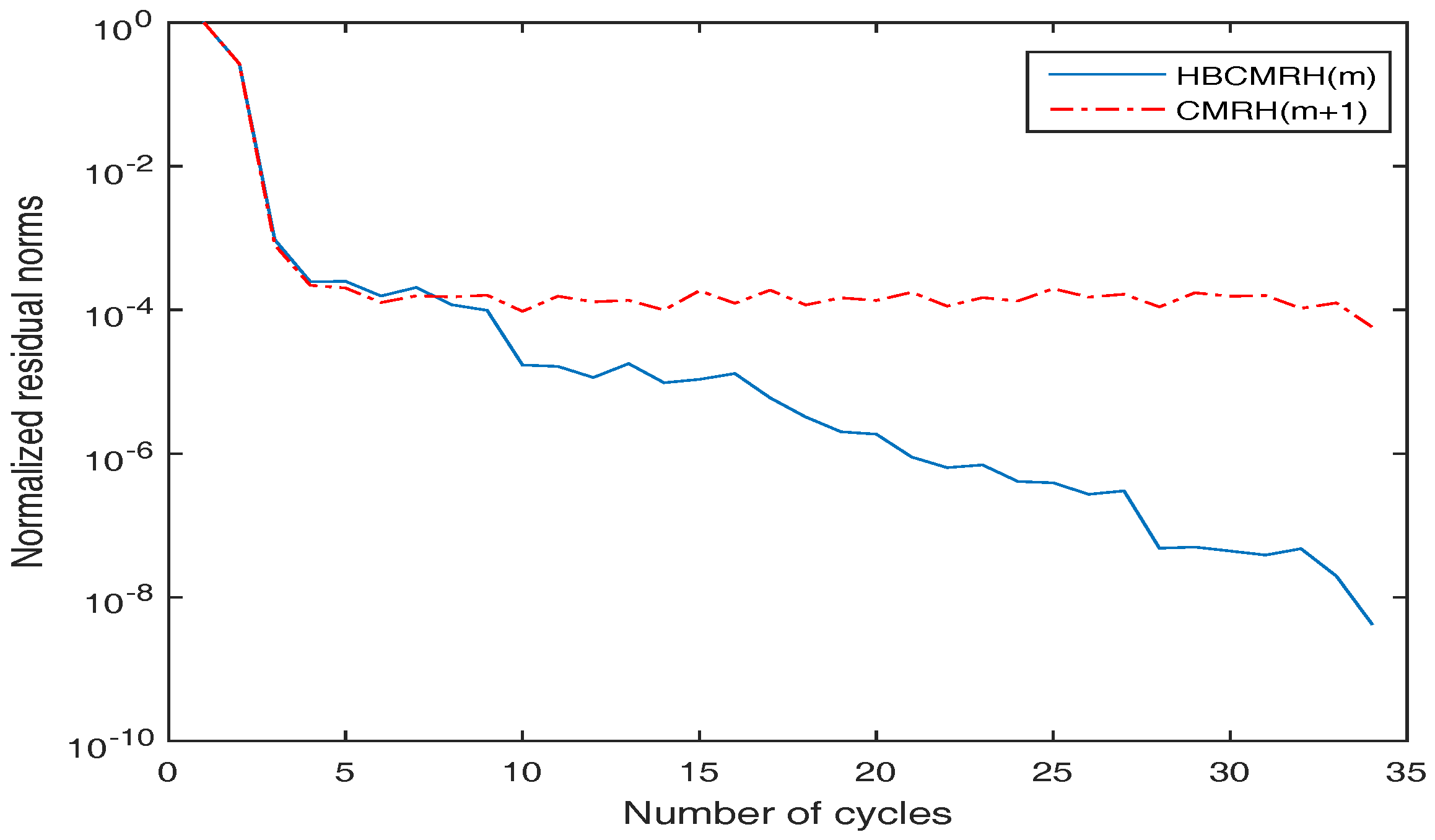
Example 1.

We first consider a $n\times n$ dense matrix

$$A=\left[\begin{array}{cccccc}1& 1& 1& \dots & 1& 1\\ {\alpha }_1& 1& 1& \dots & 1& 1\\ {\alpha }_1& {\alpha }_2& 1& \dots & 1& 1\\ ⋮& ⋮& ⋮& & ⋮& ⋮\\ {\alpha }_1& {\alpha }_2& {\alpha }_3& \cdots & {\alpha }_{n-1}& 1\end{array}\right]$$

appearing in [1] and [25] with $n=100$, $a_i=1+i\times \epsilon$, and $\epsilon ={10}^{-2}$. The right hand side $b=\mathsf{rand}(n,1)$ where $\mathsf{rand}$ is a MATLAB built-in function. In order to be fair in comparing algorithms, we tested the HBCMRH(m) method and the CMRH($m+1$) method. Recalling the remark of Algorithm 2, we know the CMRH($m+1$) method requires the same matrix-vector multiplications as HBCMRH(m), and it presents a better convergence behavior than CMRH(m). The normalized residual norms against the number of cycles of these two methods are collected in Figure 1, which clearly shows that the HBCMRH(m) method converges much faster than CMRH($m+1$). In fact, as shown in Figure 1, to reach about ${10}^{-8}$ in normalized residual norms on this example, the HBCMRH(m) method takes 34 cycles, while the CMRH($m+1$) method is seen to need much more cycles to get there.

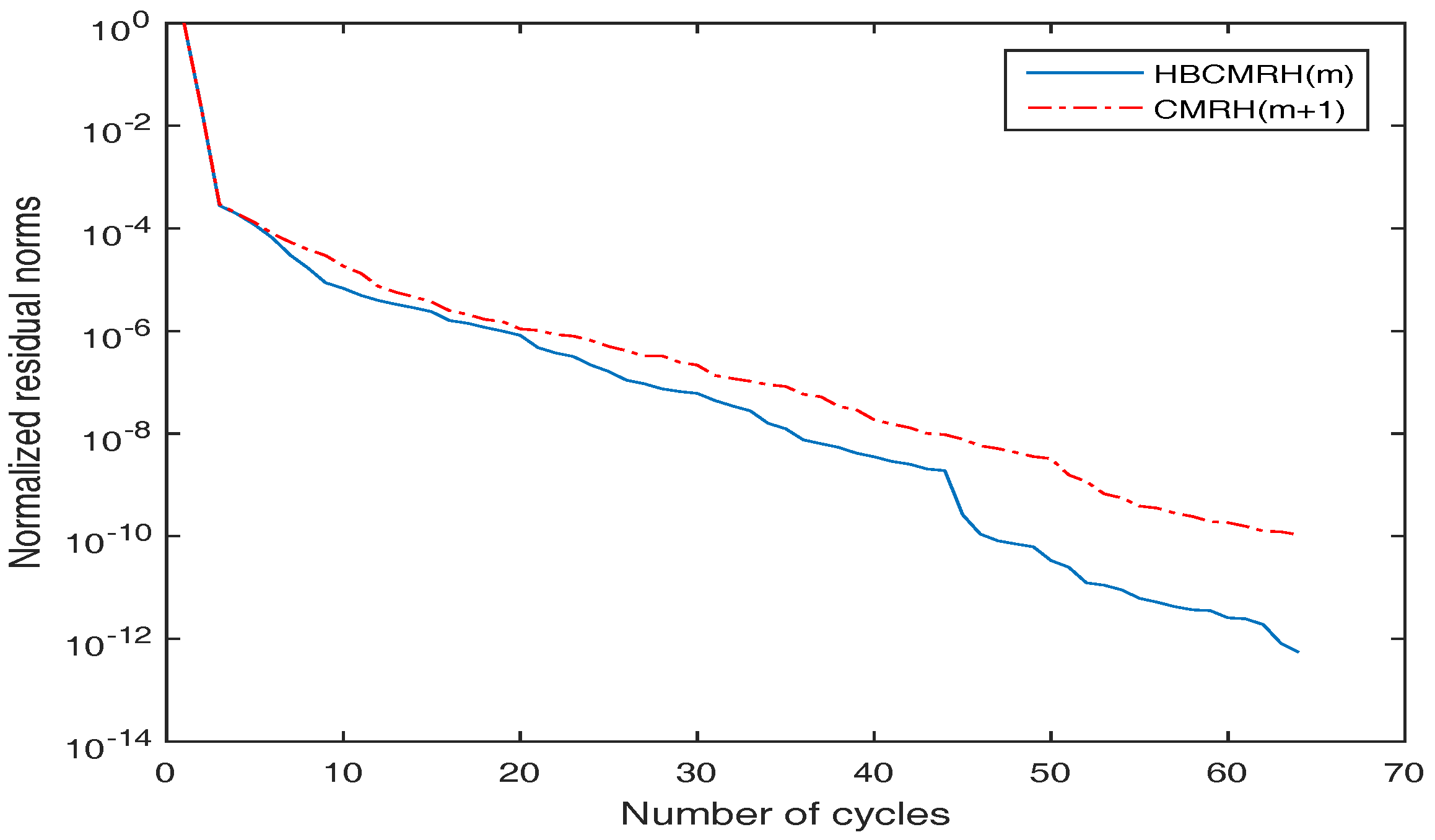
Example 2.

In this example, we consider a sparse matrix A and right hand side b which are extracted from raefsky1 taken from the University of Florida sparse matrix collection [26]. In such a problem, A is not symmetric with order $n=3242$ and contains 293,409 nonzero entries. Similarly, we compare the normalized residual norms of the HBCMRH(m) method with the CMRH($m+1$) method in Figure 2. Similar comments to the ones we made at the end of Example 1 are valid here as well.

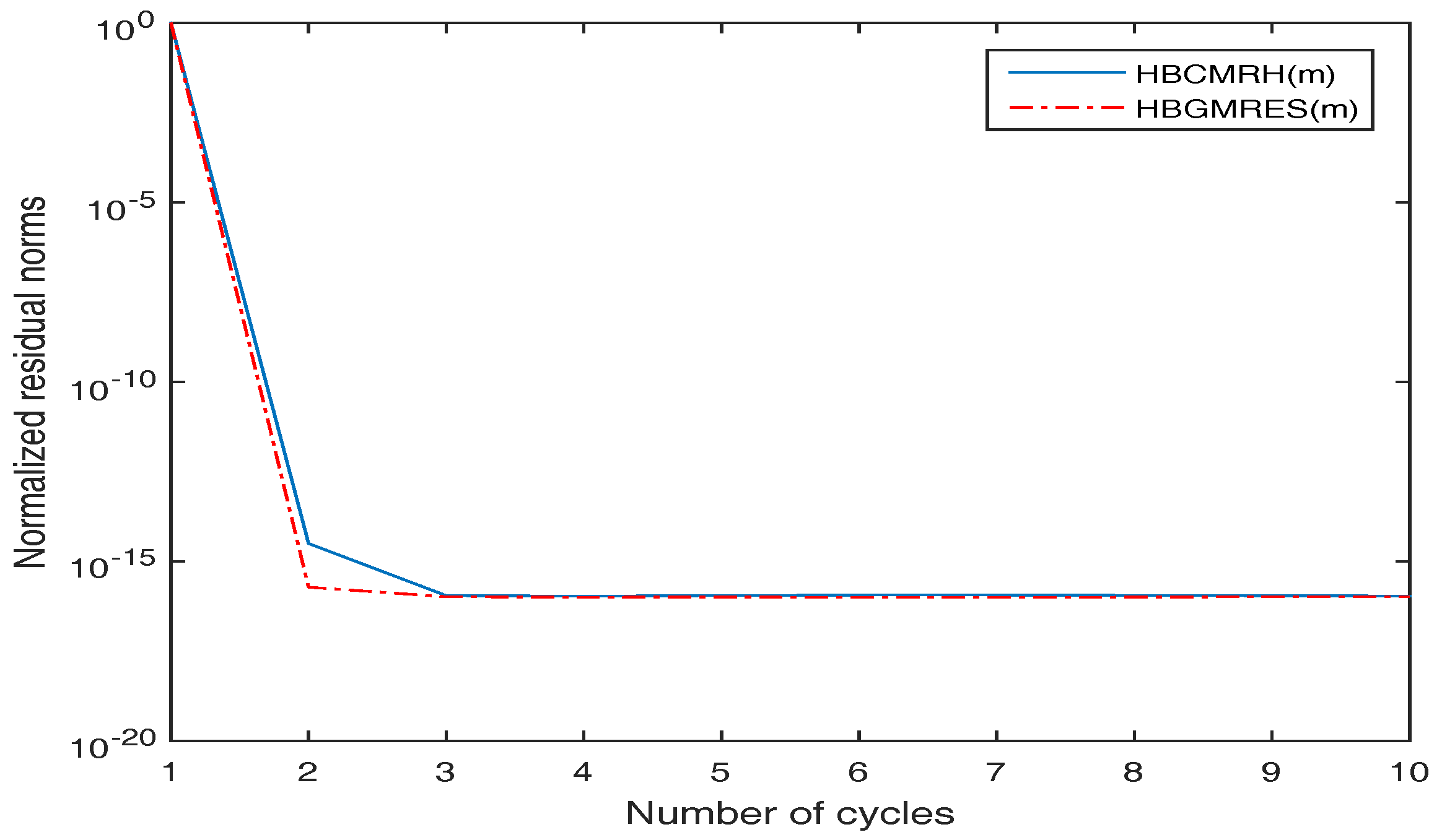
Example 3.

In this example, we use the symmetric Hankle matrix appearing in [8] with elements

$$A(i,j)=\frac{0.5}{n-i-j+1.5}$$

and $n=1000$. Let the right rand side $b=A\times \mathsf{ones}(n,1)$, where $\mathsf{ones}$ is a MATLAB built-in function. We compare the HBCMRH(m) method with the heavy ball restarted GMRES method denoted by HBGMRES(m) and compute the associated normalized residual norms in Figure 3. As shown in Figure 3, in such a case, the HBCMRH(m) and HBGMRES(m) method are competitive in the number of cycles, but less computation cost and storage requirement are needed in the HBCMRH(m) method.

4. Conclusions

In this paper, we proposed a heavy ball restarted CMRH method (HBCMRH(m) for short; i.e., Algorithm 2) for a linear system $Ax=b$. Compared to the traditional restarted CMRH method (i.e., CMRH(m)), $x_0^{(k-1)}$ is built in the search space of the HBCMRH(m) method to compute the next approximation $x_m^{(k)}$ for alleviating the loss of previous Krylov subspace. Therefore, one more matrix-vector multiplication of A is required in the HBCMRH(m) method. However, as shown in our numerical examples, HBCMRH(m) presents a better convergence behavior than CMRH($m+1$).

We have focused on the heavy ball restarted CMRH method. In fact, we can easily give the locally optimal restarted CMRH method as the locally optimal restarted GMRES method. We omit the details. In addition, while the HBCMRH(m) method has been developed for real linear systems, the algorithm can be rewritten to work for complex linear systems. This is done by simply replacing all $\mathbb{R}$ by $\mathbb{C}$ and each matrix/vector transpose by complex conjugate transpose.

References

- Sadok, H. CMRH: A new method for solving nonsymmetric linear systems based on the Hessenberg reduction algorithm. Numer. Algorithms 1999, 20, 303–321. [Google Scholar] [CrossRef]
- Heyouni, M.; Sadok, H. A new implementation of the CMRH method for solving dense linear systems. J. Comput. Appl. Math. 2008, 213, 387–399. [Google Scholar] [CrossRef]
- Saad, Y.; Schultz, M.H. GMRES: A generalized minimal residual algorithm for solving nonsymmetric linear systems. SIAM J. Sci. Comput. 1986, 7, 856–869. [Google Scholar] [CrossRef]
- Heyouni, M.; Sadok, H. On a variable smoothing procedure for Krylov subspace methods. Linear Algebra Appl. 1998, 268, 131–149. [Google Scholar] [CrossRef]
- Sadok, H.; Szyld, D.B. A new look at CMRH and its relation to GMRES. BIT Numer. Math. 2012, 52, 485–501. [Google Scholar] [CrossRef]
- Tebbens, J.D.; Meurant, G. On the convergence of Q-OR and Q-MR Krylov methods for solving nonsymmetric linear systems. Bit Numer. Math. 2016, 56, 77–97. [Google Scholar] [CrossRef]
- Duminil, S. A parallel implementation of the CMRH method for dense linear systems. Numer. Algorithms 2013, 63, 127–142. [Google Scholar] [CrossRef]
- Duminil, S.; Heyouni, M.; Marion, P.; Sadok, H. Algorithms for the CMRH method for dense linear systems. Numer. Algorithms 2016, 71, 383–394. [Google Scholar] [CrossRef]
- Lai, J.; Lu, L.; Xu, S. A polynomial preconditioner for the CMRH algorithm. Math. Probl. Eng. 2011, 2011. [Google Scholar] [CrossRef]
- Zhang, K.; Gu, C. A flexible CMRH algorithm for nonsymmetric linear systems. J. Appl. Math. Comput. 2014, 45, 43–61. [Google Scholar] [CrossRef]
- Alia, A.; Sadok, H.; Souli, M. CMRH method as iterative solver for boundary element acoustic systems. Eng. Anal. Bound. Elem. 2012, 36, 346–350. [Google Scholar] [CrossRef]
- Gu, X.M.; Huang, T.Z.; Carpentieri, B.; ImakuraWen, A.; Zhang, K.; Du, L. Variants of the CMRH method for solving multi-shifted non-Hermitian linear systems. Available online: https://arxiv.org/abs/1611.00288 (accessed on 24 February 2018).
- Gu, X.M.; Huang, T.Z.; Yin, G.; Carpentieri, B.; Wen, C.; Du, L. Restarted Hessenberg method for solving shifted nonsymmetric linear systems. J. Comput. Appl. Math. 2018, 331, 166–177. [Google Scholar] [CrossRef]
- Imakura, A.; Li, R.C.; Zhang, S.L. Locally optimal and heavy ball GMRES methods. Jap. J. Ind. Appl. Math. 2016, 33, 471–499. [Google Scholar] [CrossRef]
- Morgan, R.B. Implicitly restarted GMRES and Arnoldi methods for nonsymmetric systems of equations. SIAM J. Matrix Anal. Appl. 2000, 21, 1112–1135. [Google Scholar] [CrossRef]
- Morgan, R.B. A restarted GMRES method augmented with eigenvectors. SIAM J. Matrix Anal. Appl. 1995, 16, 1154–1171. [Google Scholar] [CrossRef]
- Morgan, R.B. GMRES with deflated restarting. SIAM J. Matrix Anal. Appl. 2002, 24, 20–37. [Google Scholar] [CrossRef]
- Bai, Z.; Li, R.C. Minimization Principle for Linear Response Eigenvalue Problem, I: Theory. SIAM J. Matrix Anal. Appl. 2012, 33, 1075–1100. [Google Scholar] [CrossRef]
- Bai, Z.; Li, R.C. Minimization Principle for Linear Response Eigenvalue Problem, II: Computation. SIAM J. Matrix Anal. Appl. 2013, 34, 392–416. [Google Scholar] [CrossRef]
- Bai, Z.; Li, R.C. Minimization principles and computation for the generalized linear response eigenvalue problem. BIT Numer. Math. 2014, 54, 31–54. [Google Scholar] [CrossRef]
- Bai, Z.; Li, R.C.; Lin, W.W. Linear response eigenvalue problem solved by extended locally optimal preconditioned conjugate gradient methods. Sci. China Math. 2016, 59, 1–18. [Google Scholar] [CrossRef]
- Knyazev, A.V. Toward the Optimal Preconditioned Eigensolver: Locally Optimal Block Preconditioned Conjugate Gradient Method. SIAM J. Sci. Comput. 2001, 23, 517–541. [Google Scholar] [CrossRef]
- Knyazev, A.V.; Argentati, M.E.; Lashuk, I.; Ovtchinnikov, E.E. Block locally optimal preconditioned eigenvalue xolvers (blopex) in hypre and petsc. SIAM J. Sci. Comput. 2007, 29, 2224–2239. [Google Scholar] [CrossRef]
- Freund, R.W.; Nachtigal, N.M. QMR: A quasi-minimal residual method for non-Hermitian linear systems. Numer. Math. 1991, 60, 315–339. [Google Scholar] [CrossRef]
- Gregory, R.T.; Karney, D.L. A Collection of Matrices for Testing Computational Algorithms; Wiley: New York, NY, USA, 1969. [Google Scholar]
- Davis, T.; Hu, Y. The University of Florida Sparse Matrix Collection. ACM Trans. Math. Softw. 2011, 38. [Google Scholar] [CrossRef]
Figure 1.
Convergence behavior of the heavy ball restarted changing minimal residual method (HBCMRH)(m) and CMRH() method.
Figure 2.
Convergence behavior of the HBCMRH(m) and CMRH() method.
Figure 3.
Convergence behavior of the HBCMRH(m) and heavy ball restarted generalized minimal residual (HBGMRES)(m) method.
© 2018 by the authors. Licensee MDPI, Basel, Switzerland. This article is an open access article distributed under the terms and conditions of the Creative Commons Attribution (CC BY) license (http://creativecommons.org/licenses/by/4.0/).
Share and Cite
MDPI and ACS Style
Teng, Z.; Wang, X. Heavy Ball Restarted CMRH Methods for Linear Systems. Math. Comput. Appl. 2018, 23, 10. https://doi.org/10.3390/mca23010010
AMA Style
Teng Z, Wang X. Heavy Ball Restarted CMRH Methods for Linear Systems. Mathematical and Computational Applications. 2018; 23(1):10. https://doi.org/10.3390/mca23010010
Chicago/Turabian StyleTeng, Zhongming, and Xuansheng Wang. 2018. "Heavy Ball Restarted CMRH Methods for Linear Systems" Mathematical and Computational Applications 23, no. 1: 10. https://doi.org/10.3390/mca23010010