1. Introduction
Tracking an object in video sequences is a key function of the intelligent surveillance system [
1,
2,
3,
4,
5,
6,
7], and it also plays important role in many other computer vision applications, including video compression, intelligent human computer interaction (HCI), and so on. During the last two decades, object tracking with visible camera has been well addressed [
8,
9,
10]. However, this is not available for the nighttime case, for that the visible camera relies heavily on the light conditions. Compared with visible cameras, the infrared imaging system is more robust to the illumination change and can work with almost no difference between daytime and nighttime. Recently, due to the quick development of computer and electronic techniques, infrared sensors have been widely utilized from military to civil fields, and object tracking in infrared sequences has become a hot research topic.
Despite that the infrared sensing system can work all the time, the main disadvantage lies in that the information it acquires is not as rich as the one from a visible camera. A visible camera can acquire visible images with ample color information, which can describe the object precisely. In contrast, the infrared camera can only record the intensity information for the working scene. Hence, in the infrared object tracking system, building an efficient model to represent the object is a critical task.
In the recent years, considerable efforts have been devoted to the infrared-based detection or tracking fields in computer vision. Similar to Comaniciu et al. [
11], Wang et al. [
12] presented a target-local background likelihood ratio based feature model to weight the histogram distribution of the target region, and this feature model was then inserted into the mean shift framework to complete the tracking process. The sparse representation technique was utilized to build the feature model of the target [
13]. In this work, they first obtained the compressed feature vector by the sparse representing method, then designed a naïve Bayes nearest neighbor classifier to track the target. Another sparse representation-based infrared target tracking algorithm was proposed in [
14], the original Haar-like features were first projected into low-dimensional features. In the next step, the L1 tracker was adopted to track the object based on compressed features. Different from the above-mentioned methods, both a saliency model and eigenspace model were employed in [
15] to serve as the observed models. This fused model was embedded in the particle filter framework to complete the infrared object tracking task. Besides single feature based infrared object tracking scheme, Wang et al. [
16] developed a multi-cue based infrared object tracking system, in this system, the intensity cue and edge cue were fused through estimating the discriminant ability for it. In [
17], an iterative particle filter was designed to implement the object tracking task, compared with the traditional particle filter, the iterative particle filter can converge much closer to the true target state with high computing efficiency.
When the tracking object is non-rigid, such as a walking person, the torso of the person is relatively stable, but the arms and legs are moving in cycles. In this case, treating the whole person as one target may lead to tracking diffusion. To enhance the performance of tracking a non-rigid object, a parts-based object representation model is employed. Adam et al. [
18] proposed a fragment-based object model by splitting the object window into multiple fragments, and each fragment was featured by a corresponding histogram. A voting scheme was then performed on each patch to determine the position and scales of the object. To reduce the computing complexity, the well-known integral histogram was utilized to extract histograms for object patches in this method. It was noticed that articulated objects, such as a human, could be approximated by several overlapped blocks, and Nejhum et al. [
19] presented an adaptive parts-based model to depict the articulated object. In this model, both the block configuration and their corresponding weights could be tuned adaptively. In the tracking process, each block associated with a histogram was extracted through the integral histogram data structure, and the object was located in a whole-image scanning manner.
In this paper, we extend the patch-based or fragment-based tracking strategy to the infrared object tracking system, and introduce an adaptively weighted patch-based infrared object tracking algorithm under the particle filtering framework. The proposed algorithm first divides the object windows into a series of non-overlapping sub-regions. After this, a particle filtering based object tracking system is realized. Meanwhile, the discriminative ability of every patch is evaluated based on the linear discriminative analysis (LDA) and particle sampling scheme.
The rest of the paper is organized as follows: in
Section 2 we make a brief introduction of the particle filter framework; then, in
Section 3, after the feature representation model is introduced, we present our new adaptive patch-based infrared object tracking scheme;
Section 4 gives the experimental results; and, finally, conclusions are made in
Section 5.
2. Particle Filter Review
In contrast to the Kalman filter, which restricts the filtering system with linear modeling and Gaussian assumptions, particle filters are often used to solve the non-linear and non-Gaussian problems. It has been proved to be an effective algorithm for object tracking [
20,
21,
22].
Particle filter is a model estimation technique based on the Monte Carlo methodologies within a Bayesian inference framework. Let Xt = {x0, x1, …, xt} and Yt = {y0, y1, …, yt} denote the state vector and the measurement up to time t, respectively. Based on the Bayesian estimation theory, the optimal estimate of xt can be deduced by the posterior mean E[xt|Yt]. Assuming that, at time t − 1, the posterior probability density function (pdf) p(xt−1|Yt−1) is known, then the posterior pdf at time t can be achieved by the following two stages:
During prediction stage, the prior
p(x
t−1|Y
t−1) is propagated to
p(x
t|Y
t−1) through a system dynamical model
p(x
t|x
t−1).
p(x
t|Y
t−1) is then be modified by the coming observation Y
t with the likelihood function L(Y
t|x
t) in the update stage. However, the integral in Equation (1) is difficult to obtain because the pdf of x is usually unknown. To avoid this problem, a particle filter employs a weighted sample set
to approximate the posterior pdf. In
S, each sample provides one candidate state of the object, with a corresponding weight
w, where
and
N is the number of particles, and the value of
w is proportional to the observation likelihood function. The expected state of the object can be estimated by:
In order to model the motion of object, a first order auto-regression (AR) dynamics model is adopted to depict the object’s translational motion. In addition to this, we also employ a random walk model to express the scale change. Let sct be the scale of the object window at time t. The random walk of sc is modeled as: , where C is a constant to control of the radius of the walk.
Suppose that a rectangular box is used to characterize the object, and then the state vector can be defined as:
where
x and
y denote the center coordinate of the rectangle,
and
give the velocities of the centric along
x and
y direction,
sx and
sy are the width and height of the rectangle. Based on the above analysis, the object state translation equation has the form of:
where
vt is stochastic noise which obey multivariate normal distribution. Matrices
A and
B are identity matrices. It is straightforward to extend this model to a higher order if a more complex dynamical model is needed.
3. The Proposed Algorithm
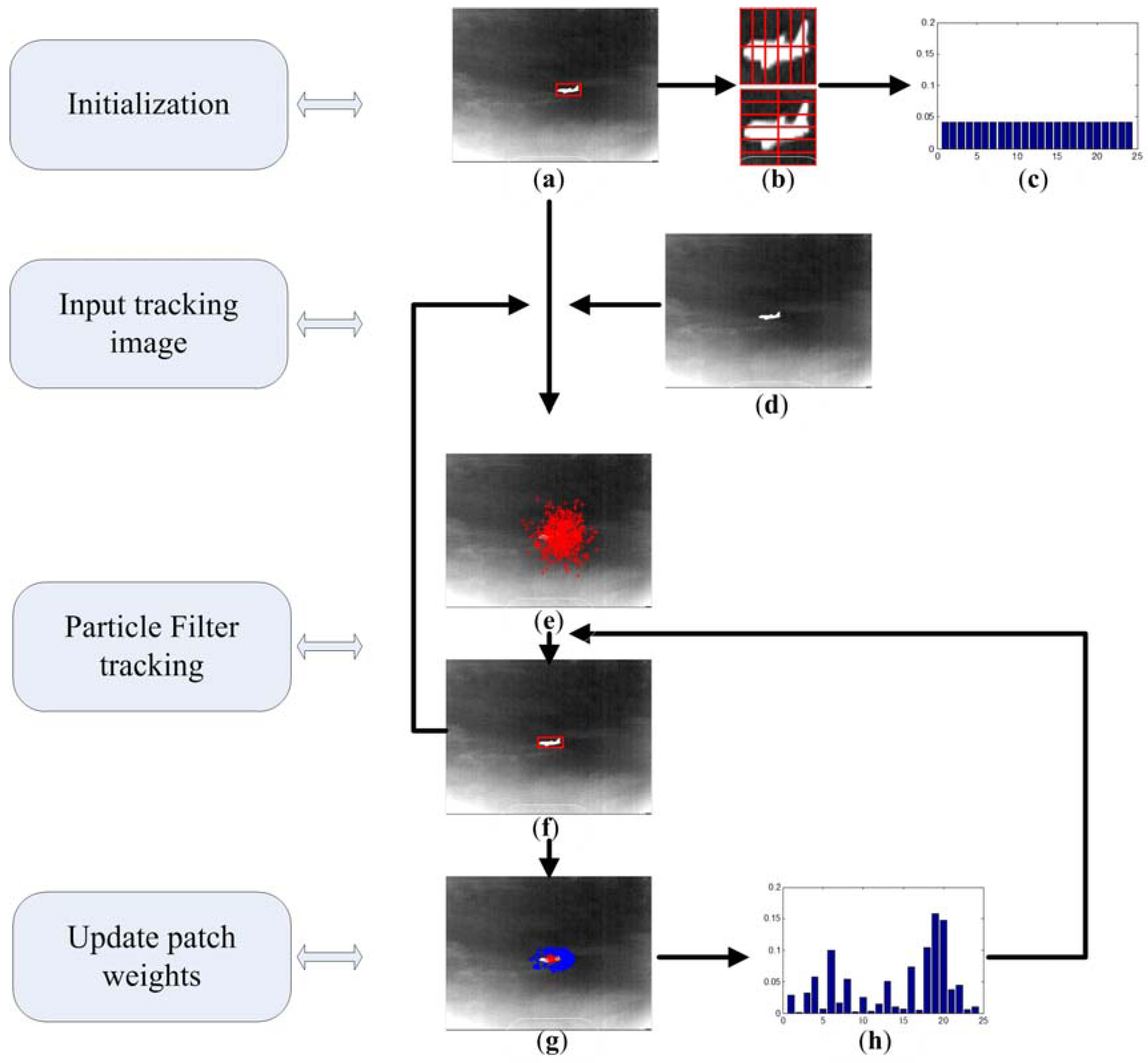
A novel patch-based infrared object tracking scheme is proposed in this section to realize the object tracking task. As can be seen in
Figure 1, in the initialization module, the target position is initialized manually on the first frame with a red bounding box (
Figure 1a). In the next step, the local region of target window is normalized to a predefined scale, and then be divided into a series of sub-regions which are shown in
Figure 1b. For each patch, a corresponding weight is assigned on it to depict its tracking ability. As described in
Figure 1c, all the weights are initialized as having equal value. When a new frame is coming, the particle filter tracking module is implemented to locate the object. This is illustrated in
Figure 1e,f. Firstly, particles are drawn according to the state transition equation. Then the current position of object is estimated by the states of particles. In the last module, the tracking performance of each sub regions is evaluated and updated. The whole tracking scheme comprises two modules: object tracking and updating weights of patches. In the object tracking module, the color particle filter framework is adopted to perform this task. When the current object state has been estimated by the particle filter, we execute the weight updating step. In this step, particles are selected to form the positive sample set and negative sample set, and these two sample sets are used to update weight of each sub-region.
3.1. Sub-Region Tracking Ability Evaluation
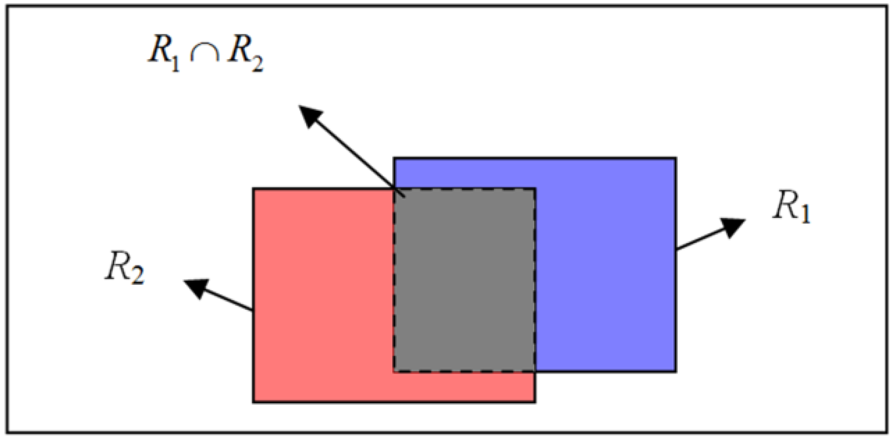
The key unit of our algorithm is the adaptive fusion of all the patches. Suppose that the current state of the object has been known, then we can measure the tracking performance of each patch based on the tracking results. In general, sub-regions which are enabled to clearly separate the object from the background have more reliable discriminative ability, thus, it should be assigned with larger weight values, and vice versa. Here, the linear discriminative analysis (LDA) technique is introduced to describe the discriminative ability of sub-regions. In the LDA, two categories of sample sets which indicate it is positive or negative should be established. In our case, we treat each particle as one sample, and the overlapping rate between particle and object is applied to decide which category the particle should belong to. As shown in
Figure 2, given two rectangle regions
R1 and
R2, the overlapping rate between them can be defined as the ratio of
and
. According to the object regions, since the positive samples describe characteristics of object, it should have large overlapping value, so as to approximate the object closely. As for the negative samples, they give characteristics of the background around the target; thus, it should have little overlapping value. However, this does not mean the negative sample should keep far away from the object, because the object only moves in a certain local region during a period of time. Based on the above analysis, the rule of selecting positive and negative samples is formulated as Equation (6), in which
is the region of particle
i.
is the region of object.
is the threshold to decide positive sample, and the negative samples are identified by two thresholds of
and
.
To measure the performance of each sub region, the LDA technique is introduced. Suppose we have built two classes of samples,
and
, based on the above presented sample selecting criterion. The means of these two sets is defined as:
The within-class scatter matrixes of them are given by:
The LDA evaluates the separability between these two classes through:
If the two groups of sample separate from each other more distinctively, then
J has a larger value. Therefore, the value of
J can be employed to indicate the discrimination between object and background. As above mentioned, the tracking window is split into several patches. Let the number of sub-regions be
M, and we choose
NP positive samples and
NN negative samples from all of the particles to build the two sample sets. For each patch P
i,
i = 1, 2, 3, …,
M, the corresponding
Ji is given by:
where:
and
Here,
is the matrix corresponding to the
ith patch in the
jth candidate region. We define the relative discriminative factors among all the patches as:
is employed to depict the discriminative property of the ith patch.
3.2. The Proposed Tracking Scheme
For the lack of visible information in infrared images, such as color, in this work the intensity feature is used to represent the tracking target. To measure the difference between candidate particles and the reference model, for each particle, the corresponding image region is normalized to have the same size as the reference region. Hence, the likelihood for patch
i can be defined as:
where
σi is the standard deviation which specifies the Gaussian noise in the measurements,
and
are the intensity matrix for
ith patch in the candidate image and reference image respectively, and the size of them have been normalized as the same. To enhance the adaptability of the tracking system, we incorporate above analyzed
into our proposed object tracking architecture. The corresponding particle weight is calculated as:
Obviously, particles with larger
w approach the target state more closely. Based on the particle filter tracking frame, the proposed tracking scheme can be summarized in Algorithm 1.
| Algorithm 1. The Proposed Tracking Algorithm |
Set the initial values: the initialization state of target x0, the number of patches M, the weight corresponding to the ith patch
for t = 1, 2, …- 1
for i = 1, 2, …, N, resample the particles: ; end for - 2
Predict the state of particle at time t: for i = 1, 2, …, N end for for i = 1, 2, …, N, normalize the weight: ; end for - 3
State estimation: - 4
Update for i = 1, 2, …, M, calculate the discriminant parameter for each patch:
end for for i = 1, 2, …, N, update : ; end for
end for |
4. Experiment Results and Analysis
In this section, we evaluate the performance of the presented algorithm through experiments on challenging infrared sequences. In the course of the experiment, four image sequences are used which are extracted from both the OTCBVS databases [
23] and datasets constructed by ourselves, a Raytheon L-3 Thermal-Eye 2000AS infrared sensors (Raytheon Company, Waltham, MA, United States) is utilized to grab 8-bit grayscale images with a resolution of 320 × 240 pixels. All of the tests are carried out on a desktop PC equipped with an Intel Core i7-4790 CPU and 8G RAM. At the first frame, the object window was drawn manually for each sequence. Both quality and quantity analysis was conducted during the experiments. We also compared the presented algorithm with three other state-of-art methods, Incremental learning for robust Visual Tracking (IVT) [
24], L1 [
25], and Compressive Tracking (CT) [
26] tracker, to depict the tracking performance more straightforwardly. Taking both the effectiveness and the computation efficiency into account, the particle number is fixed as 800 for all the tests. In our proposed tracking scheme, the value of
,
and
are experimentally set as 0.75, 0.4, and 0.1, respectively, and the target region is divided into 24 patches as illustrated in
Figure 1b. We should note that, as described in [
19], this choice of patches is arbitrary. Under this parameter setting our algorithm can run at speed of 2.5~10 fps. All of the four methods are running on MATLAB 2012a (MathWorks, Natick, MA, United States) platform.
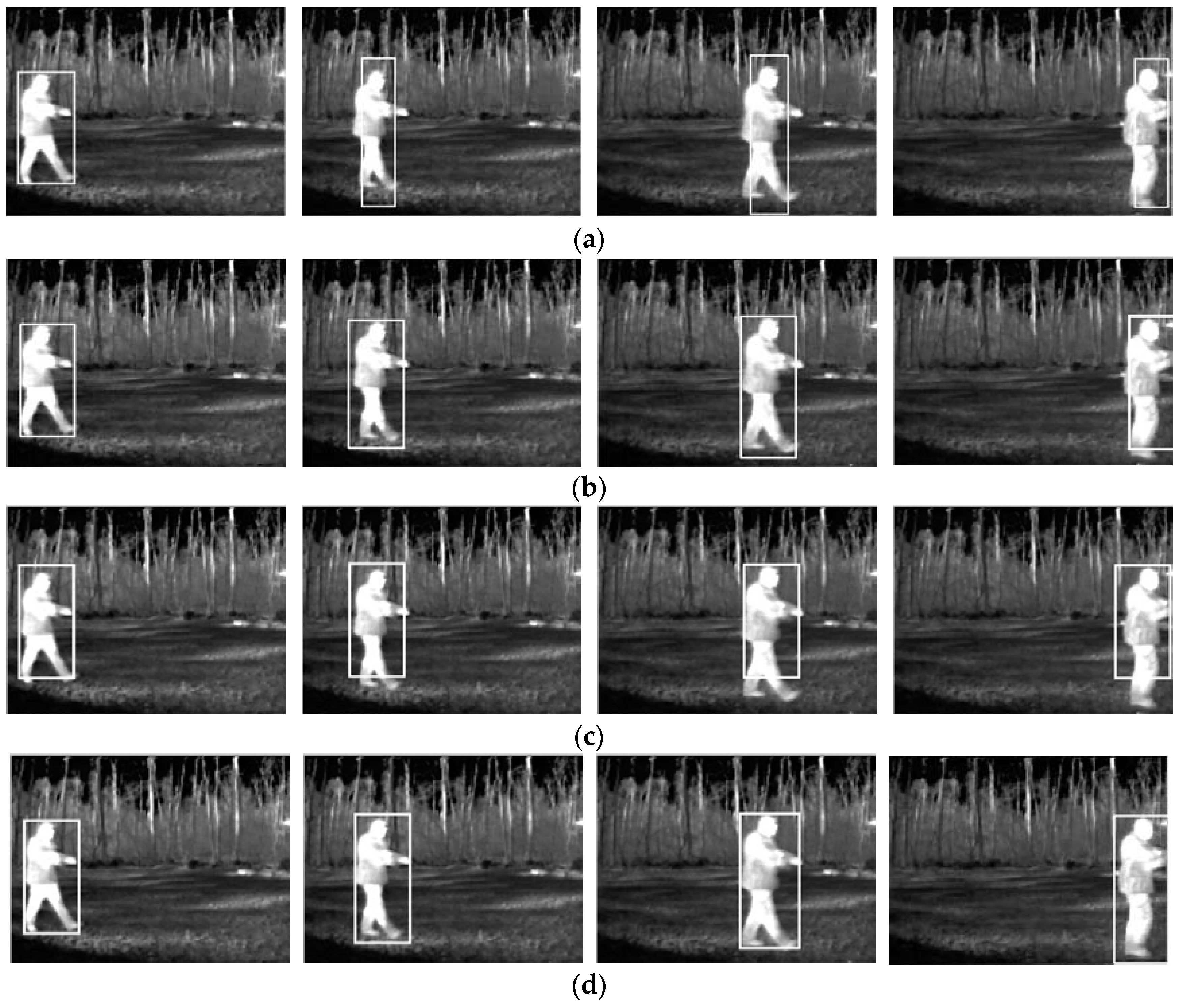
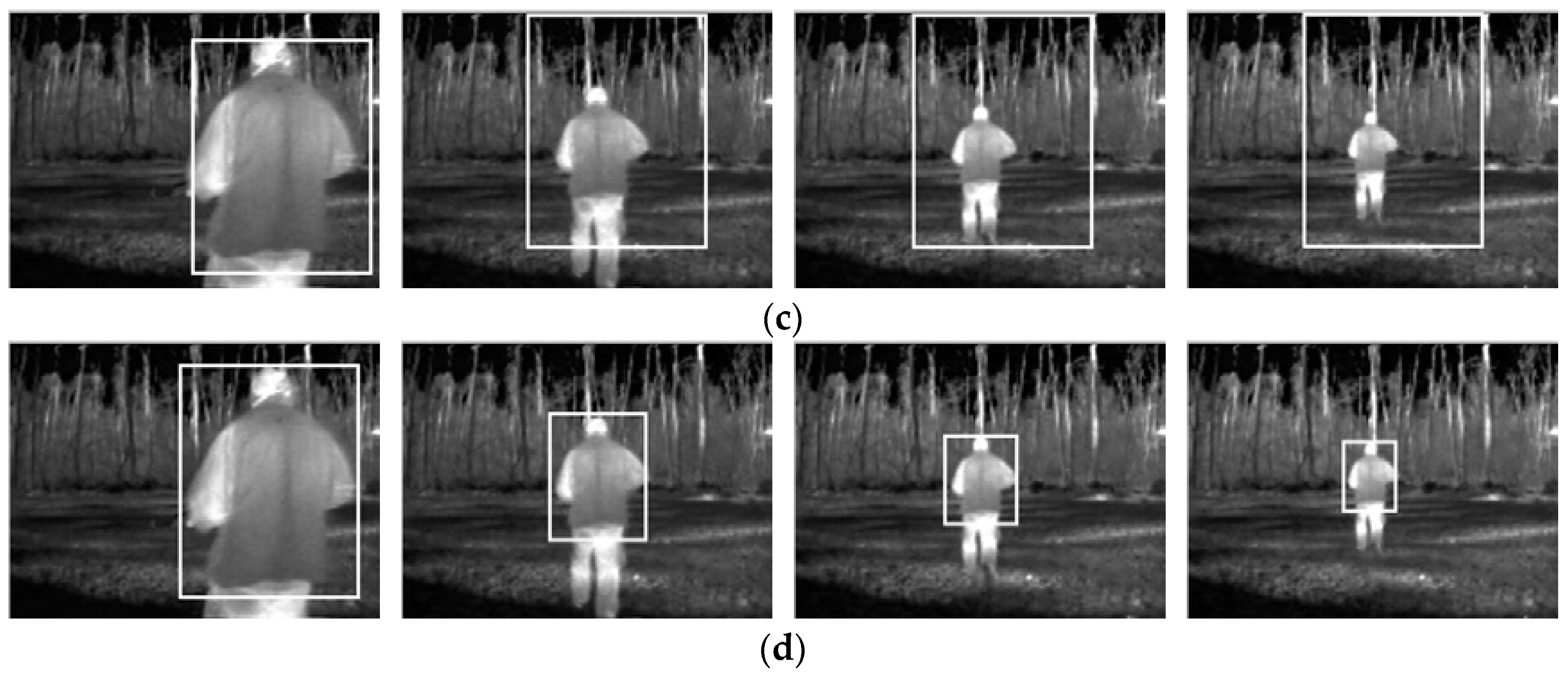
The first sequence is extracted from the familiar OTCBVS databases with a resolution of 320 × 240. In this sequence a man walks from the left side to the right side with deformation. Four sample images are given in
Figure 3, and their indices are 218, 238, 284, and 331. From top to bottom, each column in this figure is corresponding to the tracking result using IVT, L1, CT, and our algorithm, respectively. The difficulty of this sequence lies in that the shape of the target is changing with the non-rigid motion of limbs. As shown in
Figure 3, we can see that both the L1 and our proposed method enable coping with this difficulty and track the target precisely. However, the IVT and CT tracker yields considerable tracking error and that they lost some scale information during the tracking process.
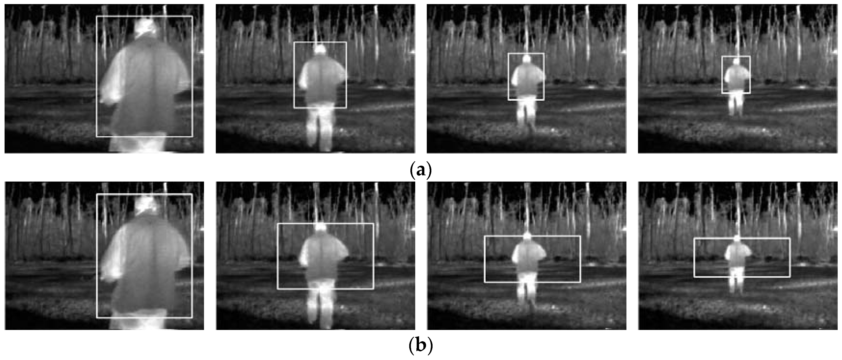
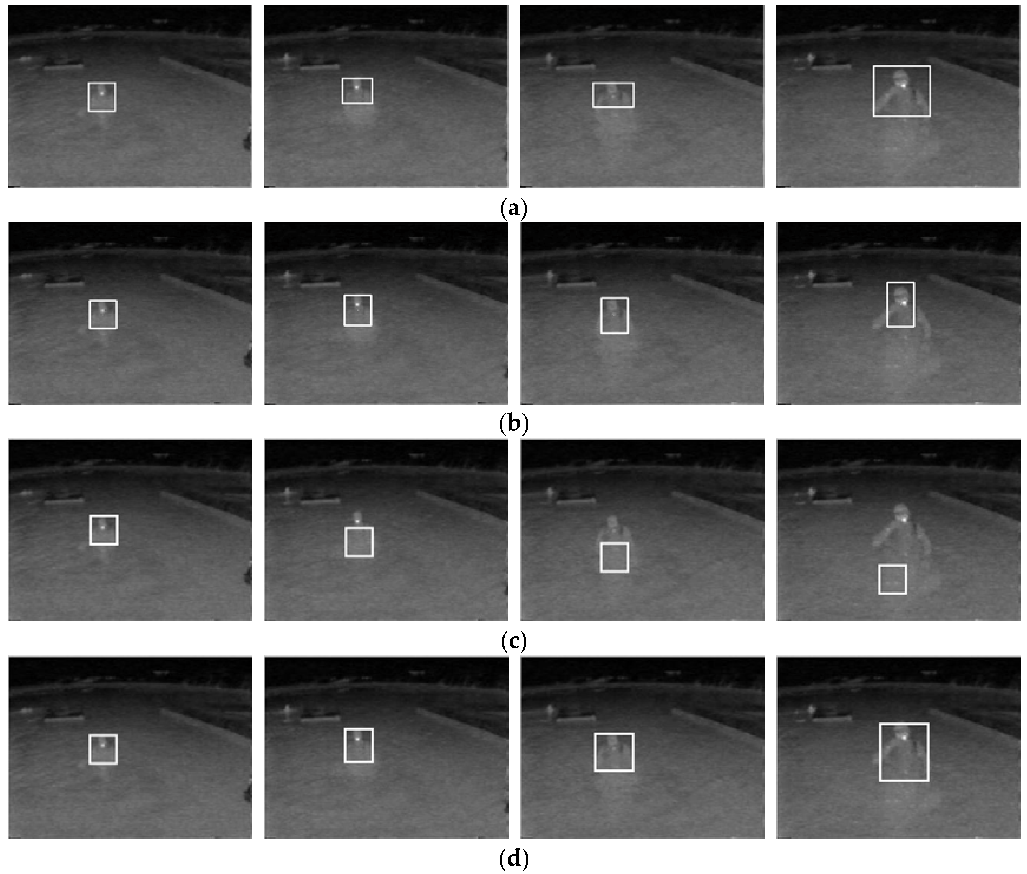
The second sequence is drawn from the Terravic Motion IR Database [
27] which is included in the OTCBVS databases with the same resolutions as sequence 1. The experimental goal of this test is to investigate the ability of handling large scale changing of the three trackers. For that, in this sequence a man walks from the near to the far with sharp variation of scale. In
Figure 4, some samples are provided; the frame indices of them from left to right are 129, 179, 222, and 261. In this test, the IVT tracker (see
Figure 4b) and our presented method (see
Figure 4d) can locate the target precisely in both position and scale. In contrast, the L1 tracker (see
Figure 4a) and the CT tracker (see
Figure 4c) failed to locate the target tightly.
An underwater sequence with low signal to noise ratio (SNR) is chosen as the third test sequence from the Terravic Motion IR Database [
27]. In this sequence, a man moves in water and the background is very cluttered, and this was monitored by an infrared sensor on the water. Four selected frames with indices of 1643, 1698, 1756, and 1853 are supplied in
Figure 5 to illustrate the tracking results. It can be observed from
Figure 5 that, besides our proposed method (see
Figure 5d), large error aroused in frame 1756 for L1 (see
Figure 5a) and frame 1853 for IVT (see
Figure 5b). As for the CT tracker, it lost the target form frame 1698. The proposed method achieved good tracking performance due to the ability of adaptive estimating the discrimination of various patches.
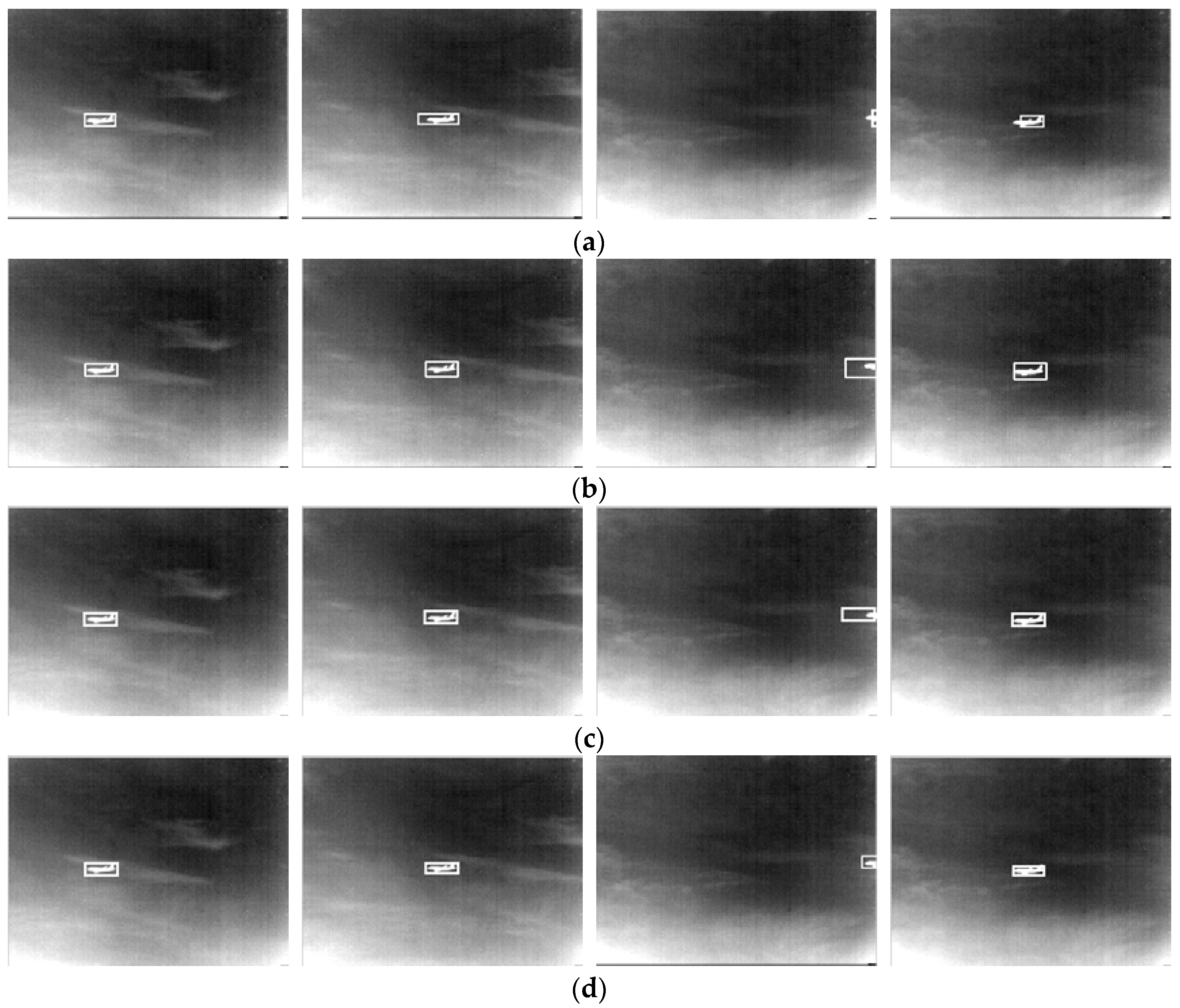
The last sequence is built by ourselves. The tracking challenge for this test lies in that the airplane had been partially flown out the camera field. In
Figure 6, four representative frames with indices of frame 1001, 1010, 1084, and 1121 are provided to display the tracking results. Each column of
Figure 6 is corresponding to one type of tracker; four columns are arranged in the same order as the past three tests. It can be observed that the L1 tracker enables coarse locating of the target, however the bounding box drifted from the target center with large errors. As for the IVT and CT tracker, despite that these could precisely locate the target in frame 1001, 1010, and 1121, but heavy bias occurred in frame 1084 due to the target partially flying out of the image. Comparing with above three trackers, our presented method was able to locate the target tightly throughout the whole sequence.
We also conduct quantitative comparison on performance of the tracking methods. In
Table 1, the average error between center of tracking results and the ground truth are given. As can be seen, our designed algorithm achieved more accurate tracking results than the L1, IVT, and CT tracker for all of the four test sequences.


