
New Scientific Contribution on the 2-D Subdomain Technique in Cartesian Coordinates: Taking into Account of Iron Parts


Abstract
:1. Introduction
1.1. Context of this Paper
- Graphical method of Lehmann (1909) [7];
1.2. State-of-the-Art: Saturation in Maxwell-Fourier Methods
- Multi-layers models (only the global saturation):
- –
- Carter’s coefficient: The slotted machine is transformed into a slotless equivalent structure by applying the usual Carter’s coefficient [28]. Generally, the armature slotting is taken into account through the SC mapping method. The analytical magnetic field distribution is determined in five or six homogeneous layers (i.e., exterior, slotless stator, winding/air-gap, magnets, and rotor) [29,30,31]. In [29], the magnetic permeabilities in stator/rotor iron cores have a constant value corresponding to linear zone of the curve. An iterative technique to include the nonlinear properties of core material has been developed in [30] (for a no-load operation) and [31] (for a load operation whose the source term in the slot caused by the armature currents is represented by a winding current region over the stator slot-isthmus). In this type of modeling, the local distribution of flux densities in the teeth and slots is neglected. However, by calculating the flux entering the stator surface from the air-gap magnetic field and thus assuming uniform distribution of flux, the flux density in middle of the stator teeth can be obtained.
- –
- Saturation coefficient: It represents the ratio between the total magnetomotive force (MMF) required for the entire magnetic circuit and the air-gap MMF [32]. The main magnetic saturation is included in the saturation factor, in an iterative way, by using the nonlinear curve. The saturation effect is accounted for by modifying the air-gap length [32,33,34] or by changing the physical properties of magnets (in this case, the saturated load operation is calculated by considering an equivalent no-load operation with a fictitious magnet having a remanent flux density that creates the same MMF as the one created by both real magnet and stator MMF) [35]. The analytical magnetic field distribution is mainly determined in one or two regions (viz., air-gap or air-gap/magnets) of slotless machines by applying the Carter’s coefficient [32]. The slotting effect can be neglected [32,35] or taken into account through the SC mapping method [33,34]. The magnetic fluxes in the stator/rotor iron cores are obtained from the air-gap magnetic field [32,33,35] or/and with a simple MEC [34]. This technique has been applied to surface-mounted/-inset magnets machines [32,33,34,35], surface-inset magnet machines [33], and others electrical machines.
- –
- Concept wave impedance: They are based on a direct solution of Maxwell’s field equations in homogeneous multi-layers of magnetic material properties, viz., the magnetic permeability and the electrical conductivity. This approach, developed by Mishkin (1953) [36], was first applied to squirrel-cage induction machine in Cartesian coordinates with three-layers (i.e., stator slotting, air-gap, and rotor slotting). It was used and enhanced by many authors, viz.,
- ∗
- simplification of the electromagnetic theory [37];
- ∗
- extended with an infinite number of layers [38];
- ∗
- converted into equivalent circuits and terminal impedance [39];
- ∗
- included the curvature effect with the magnetizing current [40];
- ∗
- ∗
- ∗
- taking account of the slot-opening effect [45], i.e., the multi-layers model is combined with the subdomain technique for slotted structures by assuming infinitely permeable tooth-tips;
- ∗
- –
- Convolution theorem: The electrical machine is divided into an infinite number of (in)homogeneous layers. The permeability in the stator and/or rotor slotting is represented by a complex Fourier series along the direction of permeability variation The permeability variation in the direction of the periodicity is directly included into the solution of the magnetic field equation. The resulting formulation, based on a direct solution of Maxwell’s field equations using the Cauchy’s product theorem (i.e., the discrete convolution of two infinite series), is completely defined in terms of complex Fourier series [47]. Recently, Djelloul et al. (2016) [48] extended this modeling taking into account the nonlinear curve in each soft-magnetic section by an iterative procedure. For the moment, this technique has been applied to a switched reluctance machine [48] and a synchronous reluctance machine [49].
- Eigenvalues model (only the global saturation): The electromagnetic field can be solved directly by applying the method of Truncation Region Eigenfunction Expansions (TREE) [50]. The iron cores have finite magnetic permeability and finite height/width. The studied domains can be (non)conductive. The boundary value problem is formulated in terms of the magnetic vector potential, which is expanded in a series of appropriate eigenfunctions. The unknown coefficients of the series are computed by solving a matrix system (by using a standard method such as the lower upper decomposition), which is formed by applying the usual interface conditions. The corresponding eigenvalues are the real roots of a function with the geometrical and the magnetic permeability of the core as parameters. Nevertheless, an iterative numerical method (e.g., the bisection [50] and Newton-Raphson [51] method) is always adopted to compute the discrete eigenvalues in both the odd and even parity solutions. For the moment, this technique has been widely applied to the non-destructive testing of conductive materials (e.g., for the I-cored [50] and E-cored [52,53] probes, for a long coil with a slot in a conductive plate [51], etc.).
- Hybrid models (the local/global saturation): The analytical solution can be combined with numerical methods [54,55,56,57] or (non)linear MEC [58,59,60,61,62,63,64,65,66,67]. Usually, the analytical solution is established in uniform regions of very low permeability (e.g., air-gap, and magnets) and other methods are sought in regions where magnetic saturation cannot be neglected (i.e., the stator and/or rotor iron cores).
1.3. Objectives of this Paper
2. A 2-D Subdomain Technique of Magnetic Field
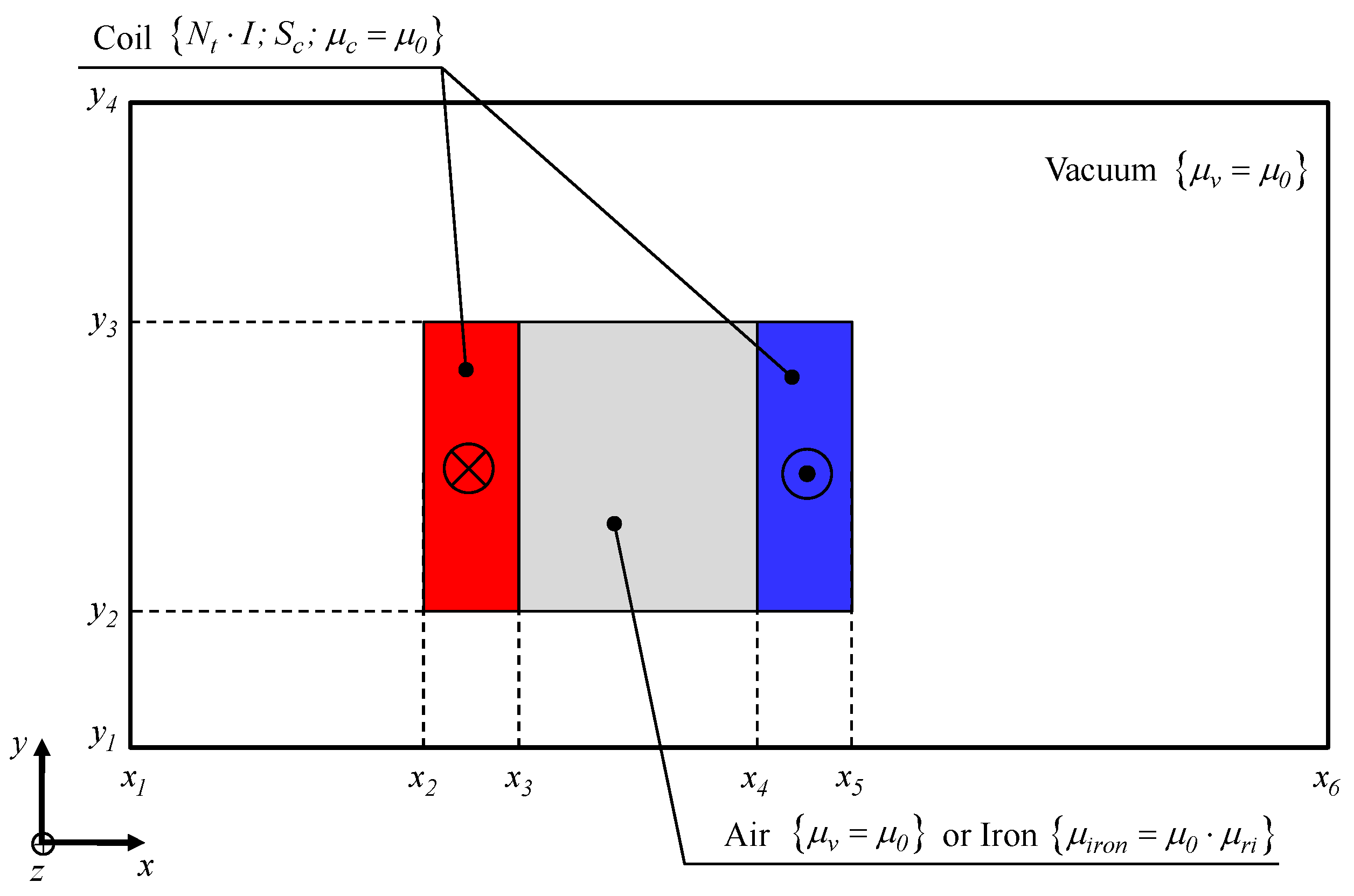
2.1. Problem Description and Assumptions
- The end-effects are neglected (i.e., that the magnetic variables are independent of z);
- The electrical conductivities of materials are assumed to be null (i.e., the eddy-currents induced in the copper/iron are neglected);
- The magnetic materials are considered as isotropic (i.e., the permeability can be assumed the same in the two directions);
- The effect of global saturation is taken into account with a constant magnetic permeability corresponding to linear zone of the curve (i.e., the initial magnetization curve).
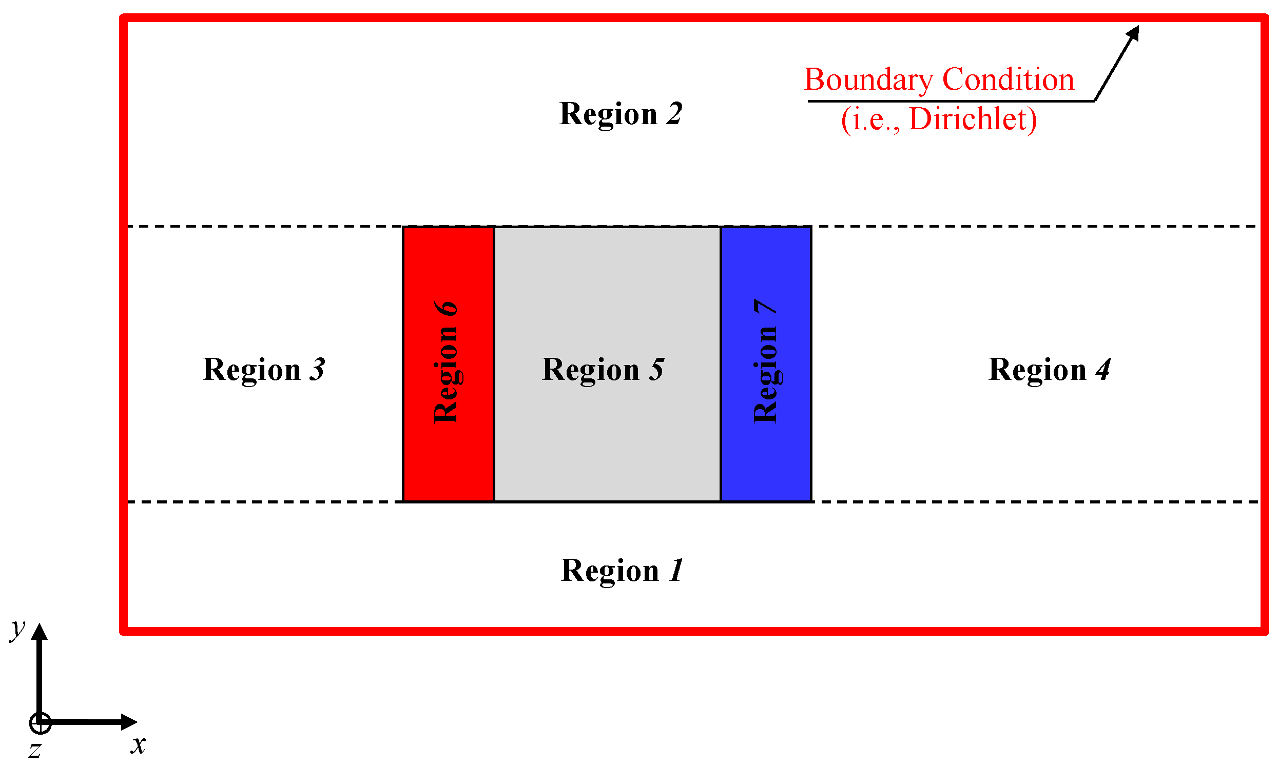
2.2. Problem Discretization in Subdomains
- Region 1 with ;
- Region 2 with ;
- Region 3 with ;
- Region 4 with .
- Region 6 with ;
- Region 7 with .
2.3. Governing Partial Differential Equations in Cartesian Coordinates
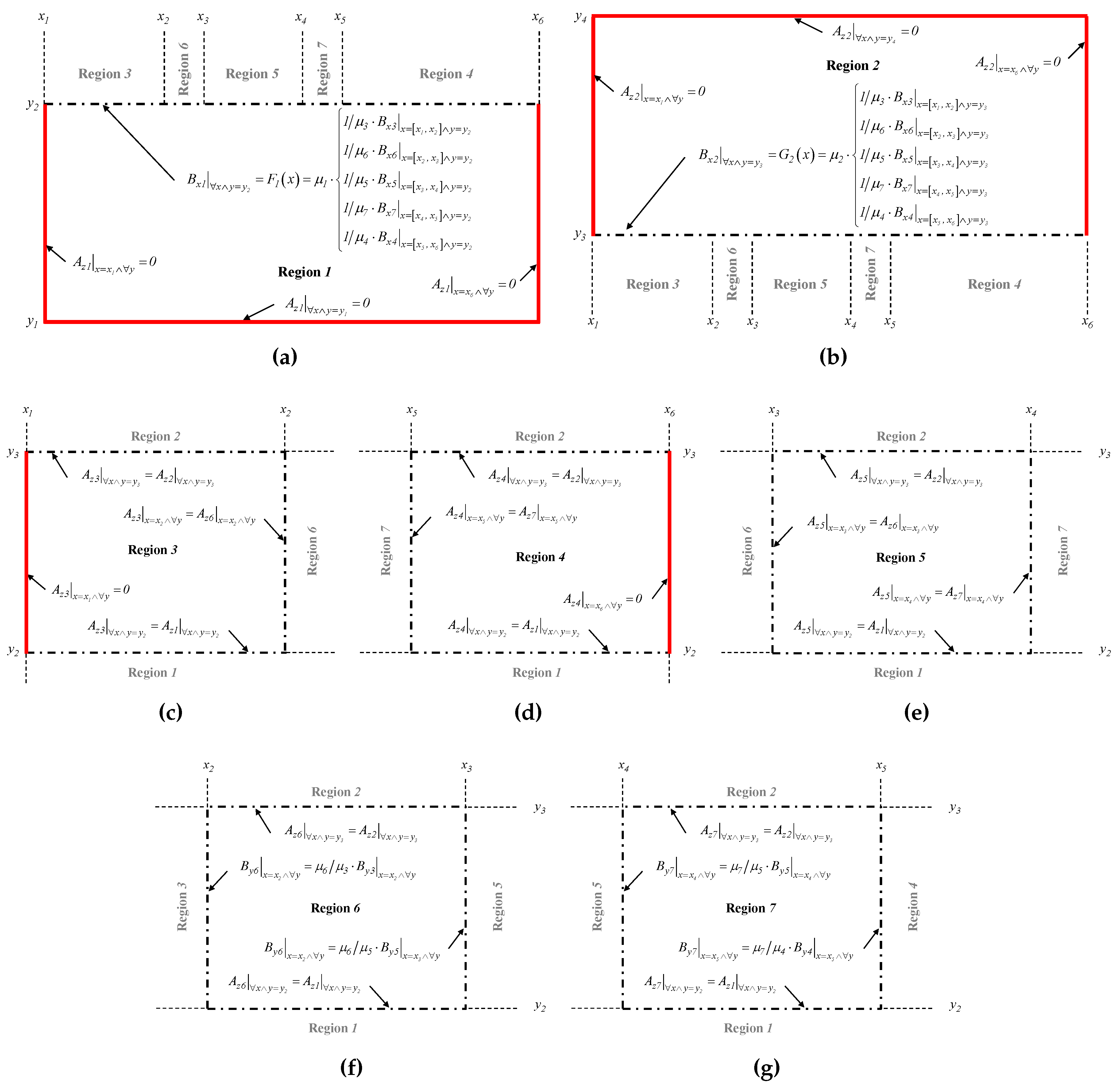
2.4. Boundary Conditions
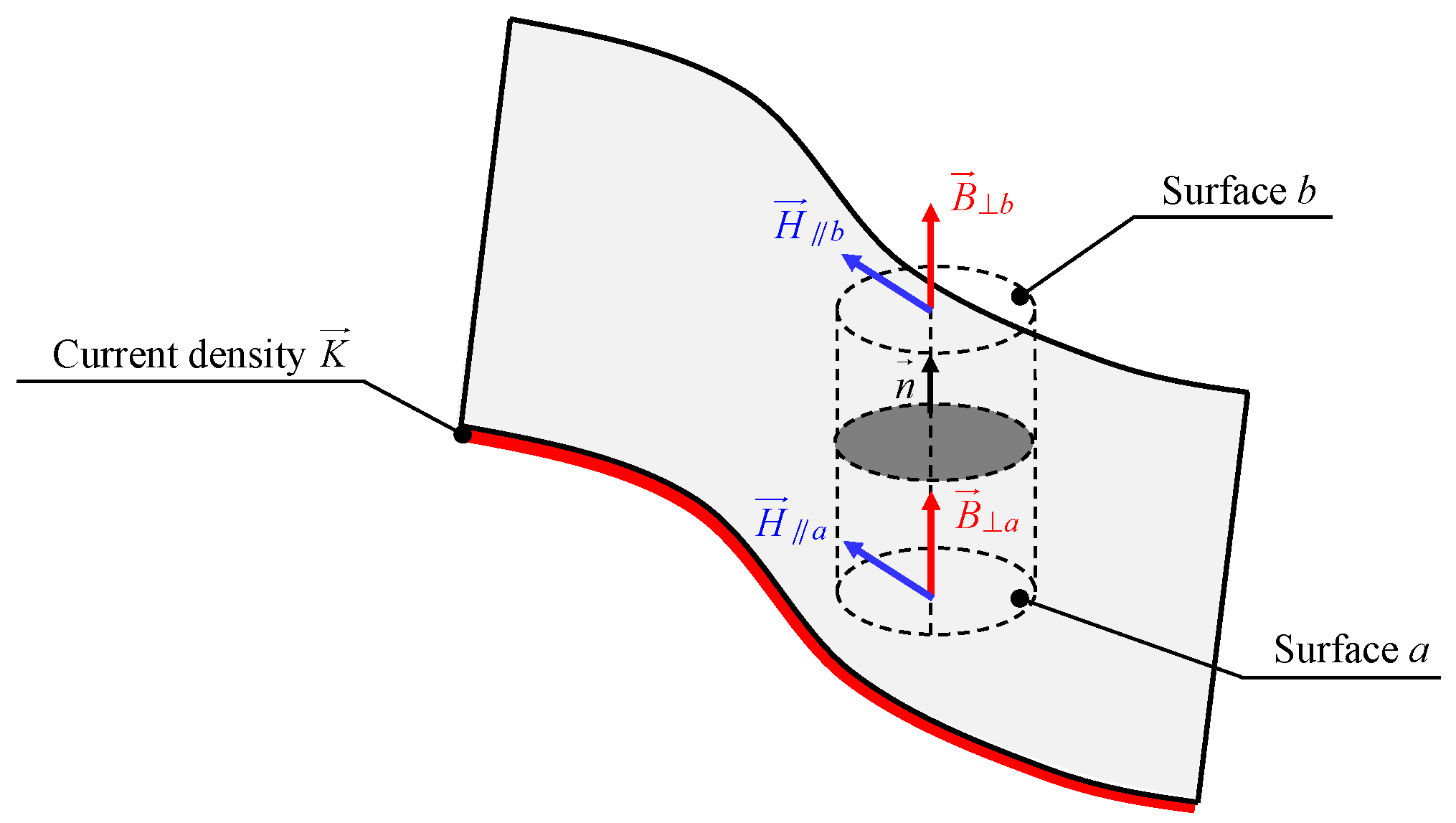
2.4.1. Reminder on the Boundary Conditions at the Interface of Two Surfaces
2.4.2. Application to the Air- or Iron-Cored Coil
2.5. General Solutions
2.5.1. Region 1
2.5.2. Region 2
2.5.3. Region 3
2.5.4. Region 4
2.5.5. Region 5
2.5.6. Region 6
2.5.7. Region 7
2.6. Solving of Linear System
2.7. Numerical Problems: Harmonics and Ill-Conditioned System
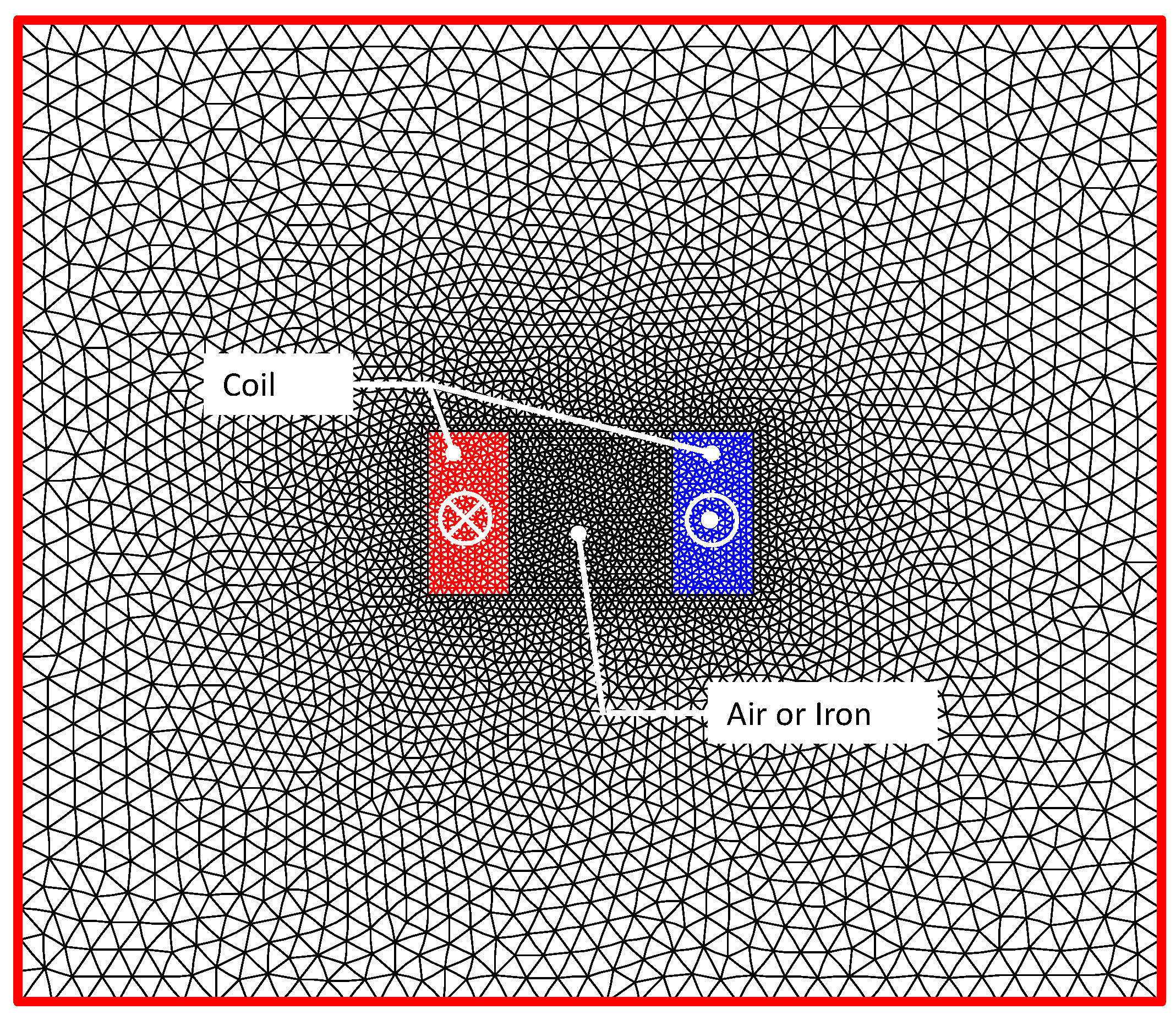
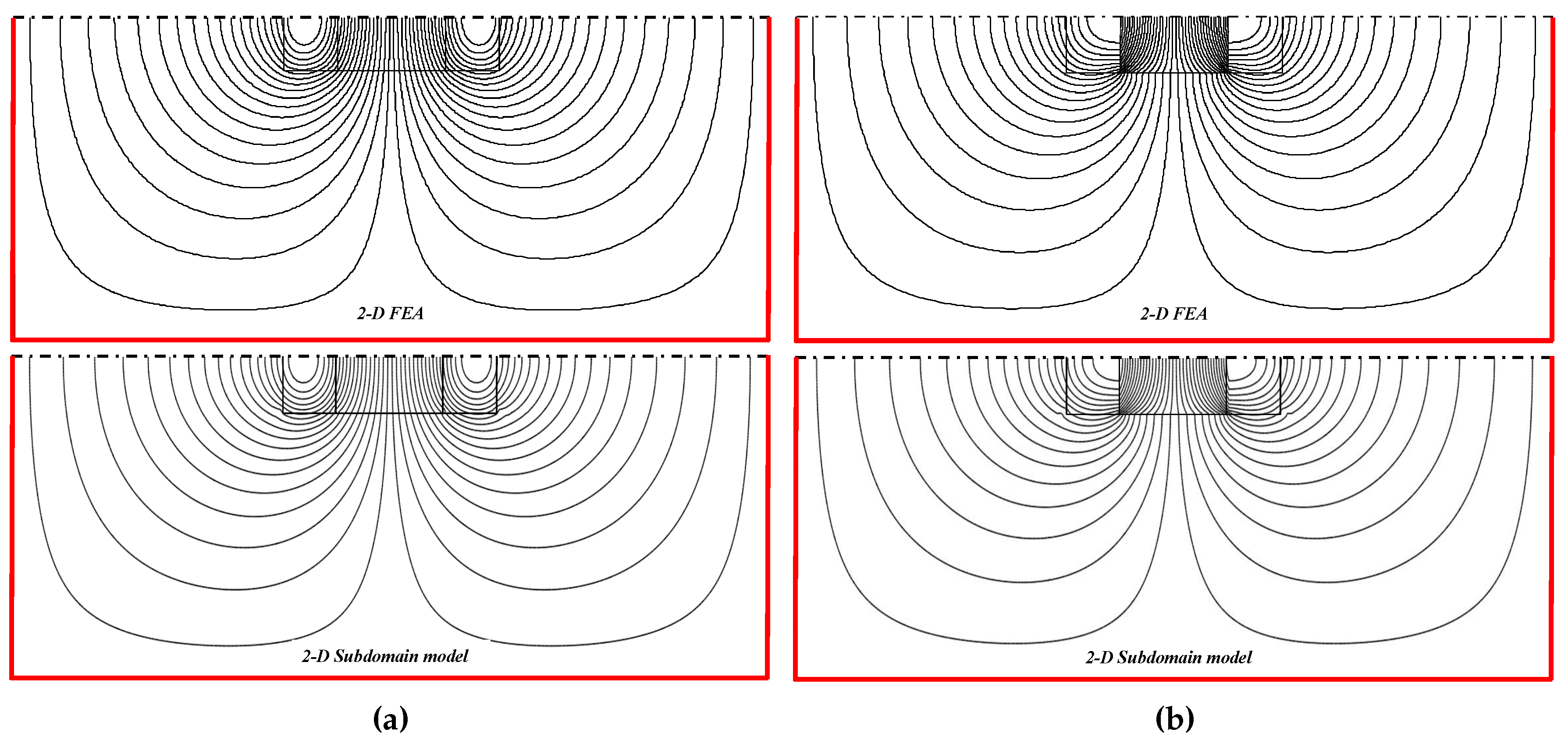
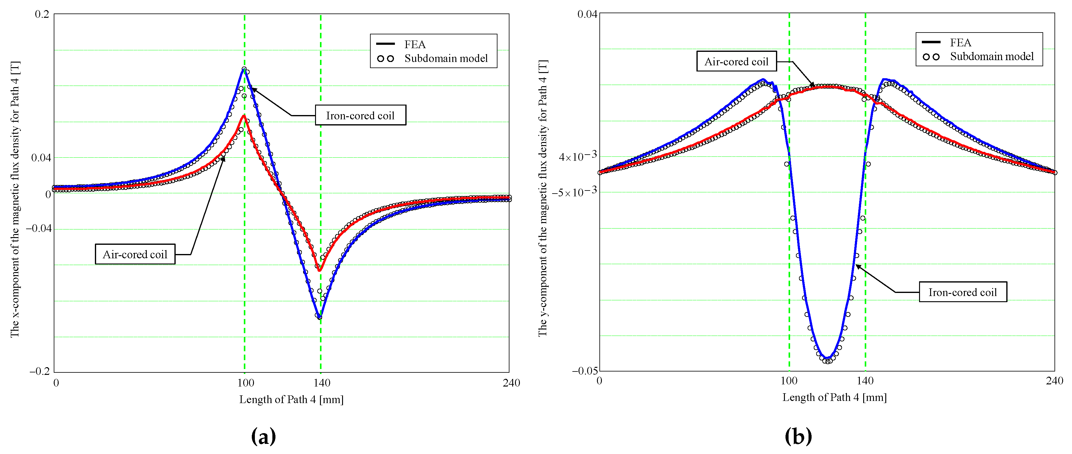
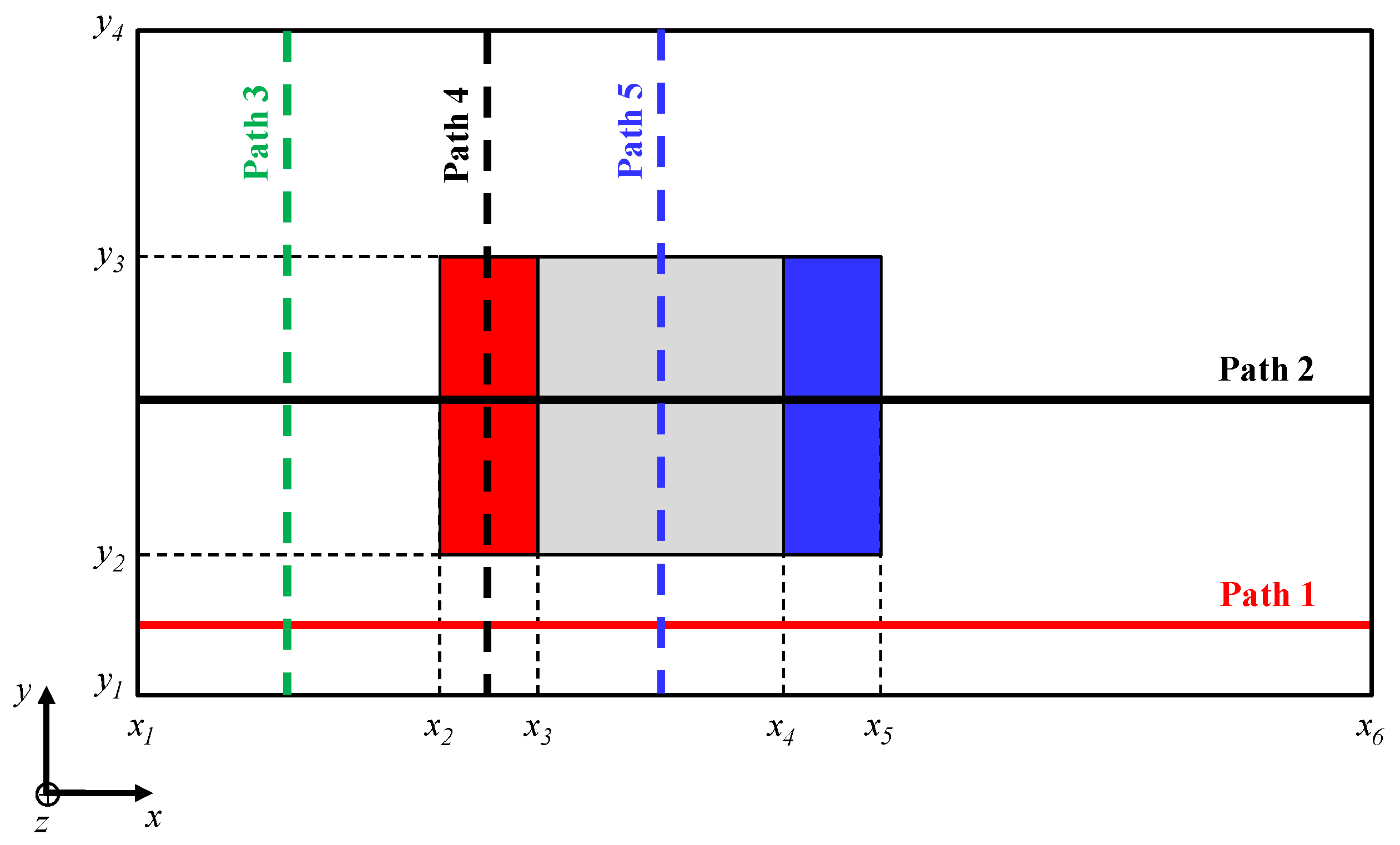
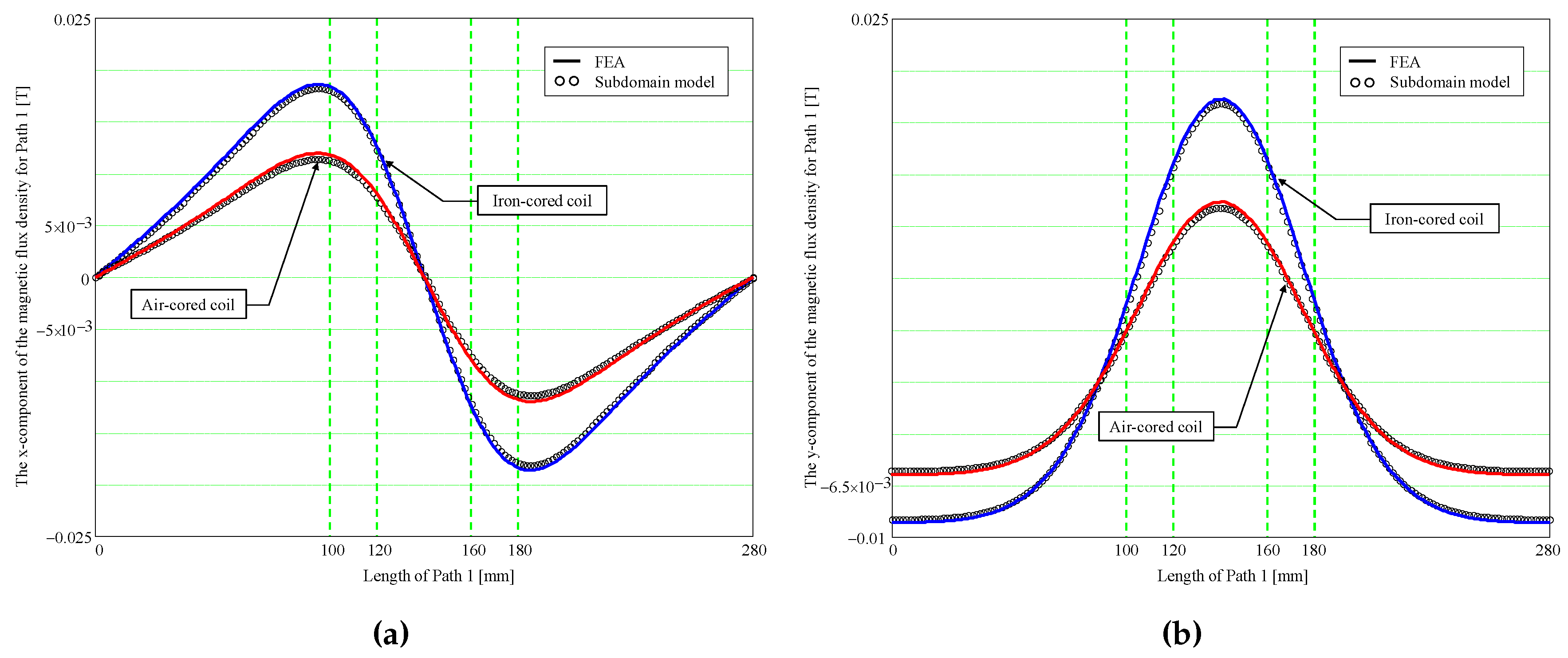
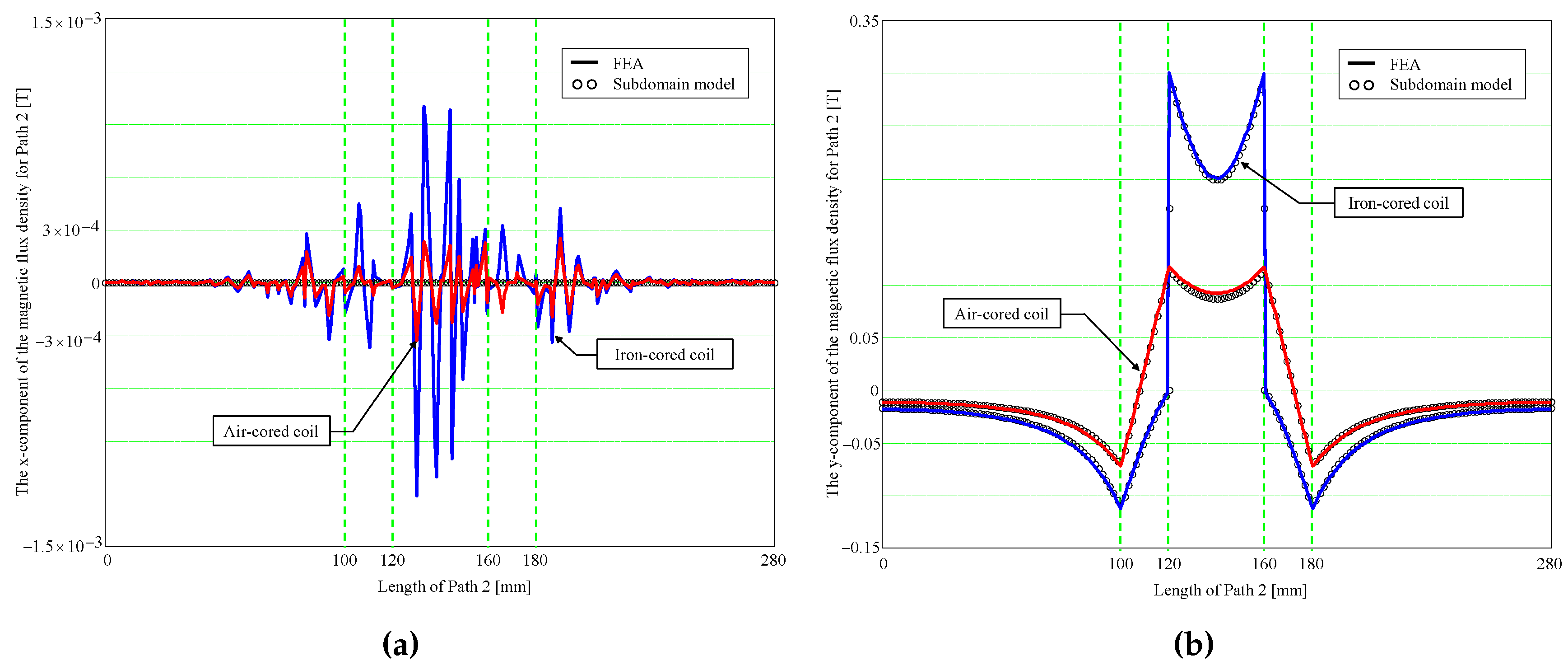
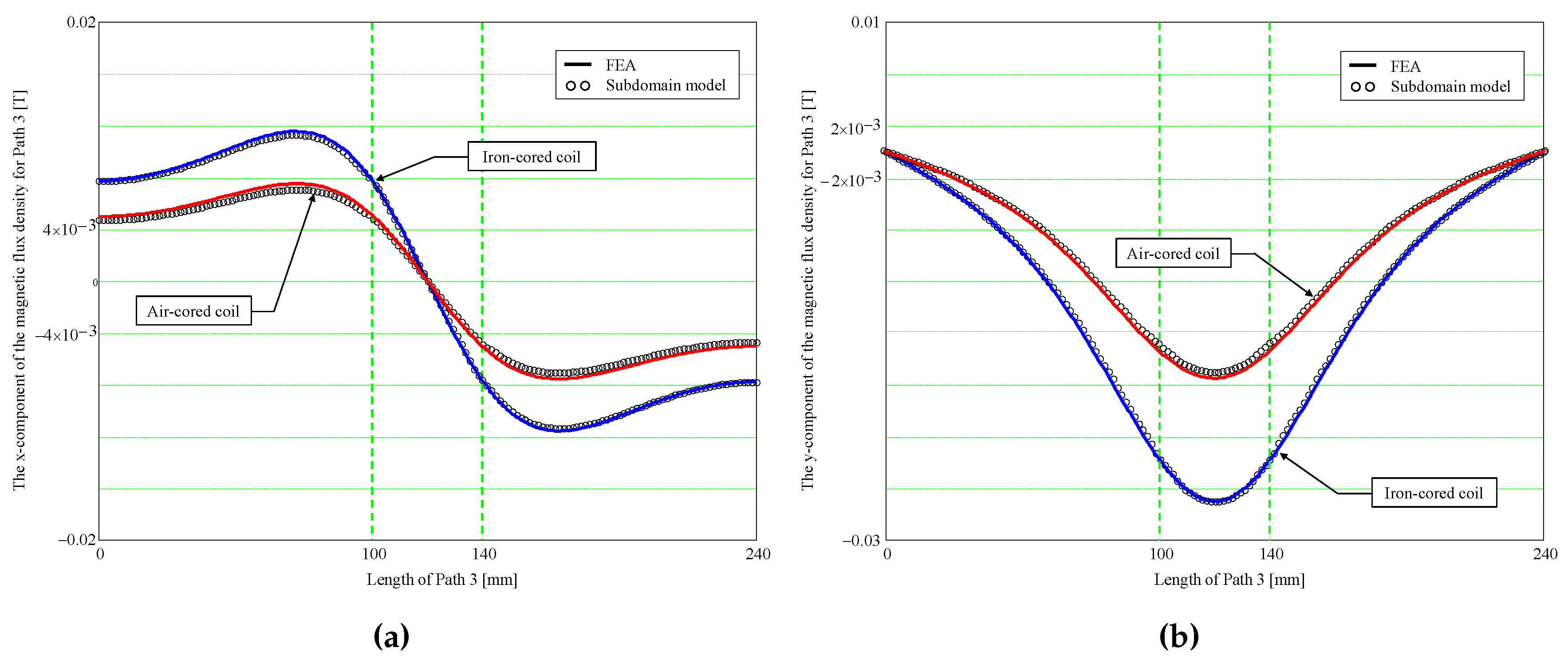
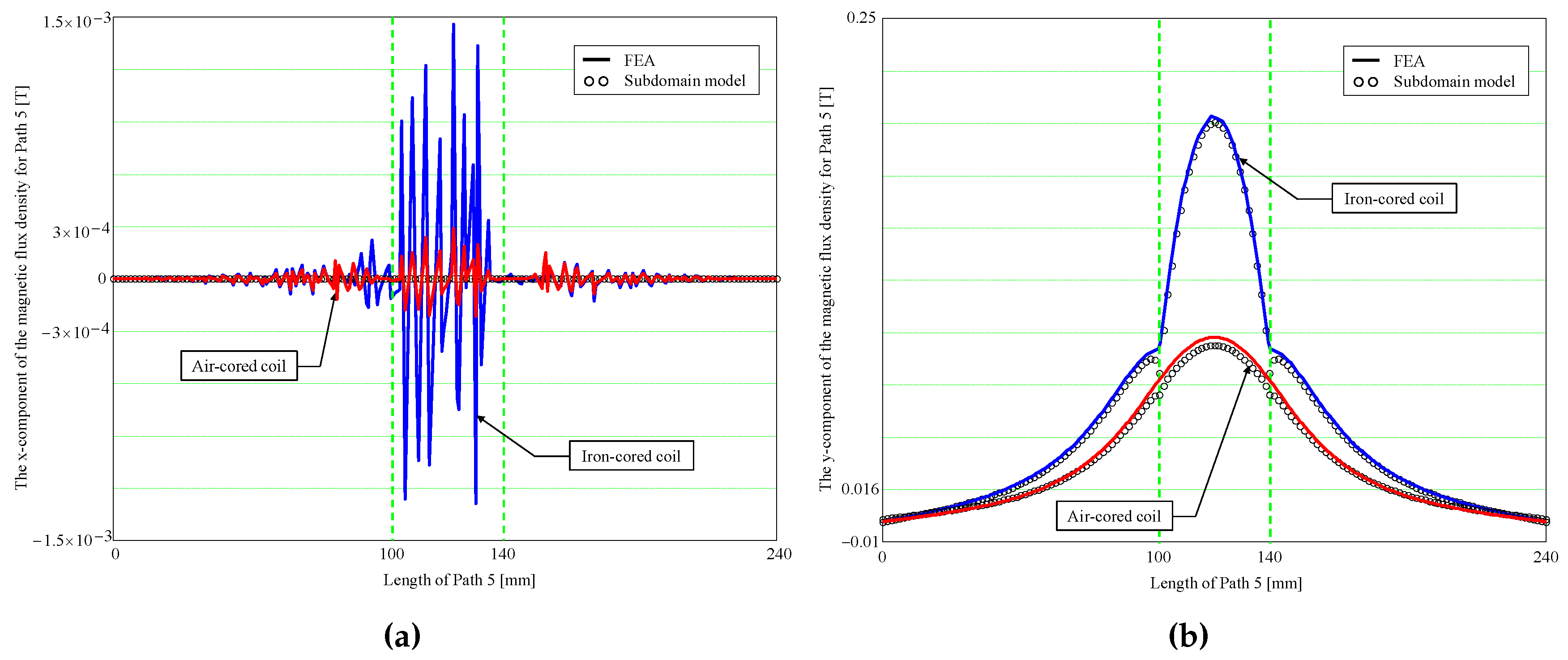
3. Comparison of the Semi-Analytic and Finite-Element Calculations
3.1. Introduction
3.2. Results Discussion
4. Conclusions
Author Contributions
Conflicts of Interest
Appendix A The 2-D Magnetostatic General Solution in Cartesian Coordinates
Appendix A.1 Governing Partial Differential Equations (EDPs)
Appendix A.2 General Solution
Appendix B Simplification of Laplace’s Equations According to Imposed Boundary Conditions
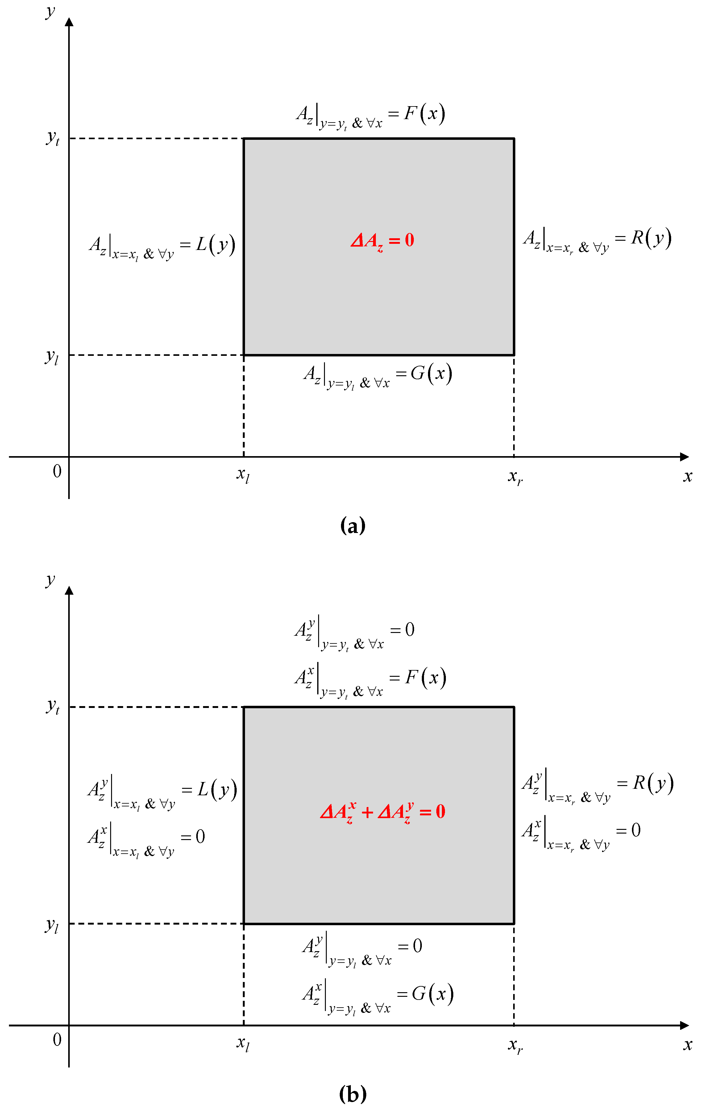
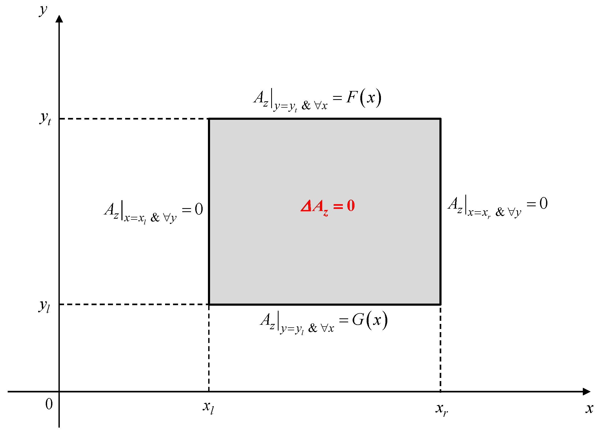
Appendix B.1 Case-Study No 1: Az imposed on all edges of a region


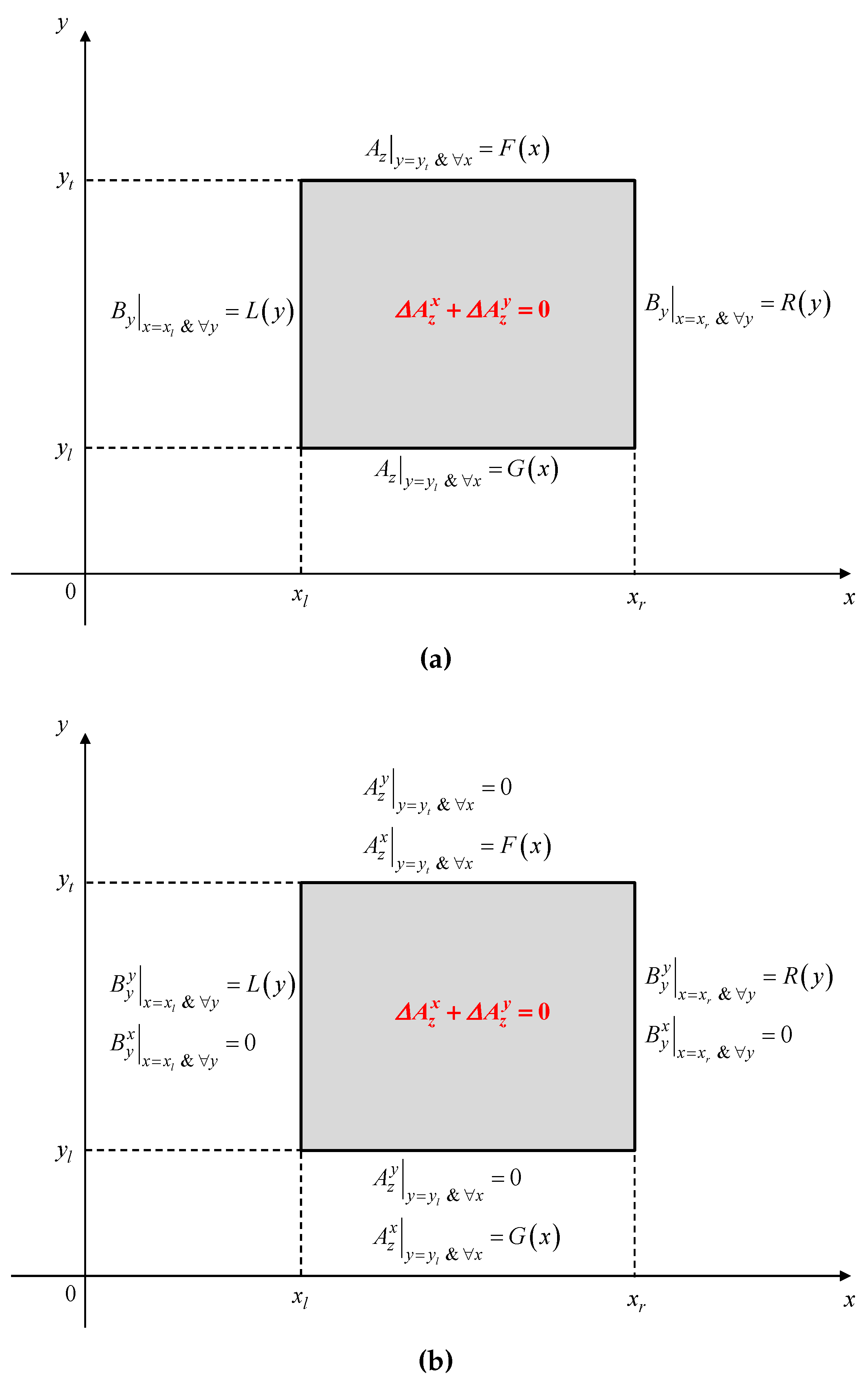
Appendix B.2 Case-Study No 2: By and Az are respectively imposed on x- and y-edges of a region

Appendix C Elements of Linear Systems
Appendix C.1 Simplifying Function of General Integrals
Appendix C.2 Expression of for Region 1
Appendix C.3 Expression of for Region 2
Appendix C.4 Expression of , and for Region 3
Appendix C.5 Expression of , and for Region 4
Appendix C.6 Expression of , , and for Region 5
Appendix C.7 Expression of , , , , and for Region 6
Appendix C.8 Expression of , , , , and for Region 7
References
- Yilmaz, M.; Krein, P.T. Capabilities of finite element analysis and magnetic equivalent circuits for electrical machine analysis and design. In Proceedings of the 2008 Power Electronics Specialists Conference (PESC), Rhodes, Greece, 15–19 June 2008.
- Dubas, F.; Espanet, C. Analytical solution of the magnetic field in permanent-magnet motors taking into account slotting effect: No-load vector potential and flux density calculation. IEEE Trans. Magn. 2009, 45, 2097–2109. [Google Scholar] [CrossRef]
- Zhu, Z.Q.; Wu, L.J.; Xia, Z.P. An accurate subdomain model for magnetic field computation in slotted surface-mounted permanent-magnet machines. IEEE Trans. Magn. 2010, 46, 1100–1115. [Google Scholar] [CrossRef]
- Rahideh, A.; Korakianitis, T. Analytical calculation of open-circuit magnetic field distribution of slotless brushless PM machines. Electr. Power Energy Syst. 2012, 44, 99–114. [Google Scholar] [CrossRef]
- Tiegna, H.; Amara, Y.; Barakat, G. Overview of analytical models of permanent magnet electrical machines for analysis and design purposes. Math. Comput. Simul. 2013, 90, 162–177. [Google Scholar] [CrossRef]
- Curti, M.; Paulides, J.J.H.; Lomonova, E.A. An overview of analytical methods for magnetic field computation. In Proceedings of the Tenth International Conference on Ecological Vehicles and Renewable Energies (EVER), Monte Carlo, Monaco, 31 March–2 April 2015.
- Lehmann, T. Méthode graphique pour déterminer le trajet des lignes de force dans l’air. Revue d’Électricité: La Lumière Électrique 1909, 43–45, 103–110; 137–142; 163–168. [Google Scholar]
- Flux2D. General Operating Instructions; Version 10.2.1; Cedrat S.A. Electrical Engineering: Grenoble, France, 2008. [Google Scholar]
- Jin, J. The Finite Element Method in Electromagnetic, 2nd ed.; John Wiley & Sons, Inc.: New York, NY, USA, 2002. [Google Scholar]
- Stoll, R.L. The Analysis of Eddy Currents; Clarendon Press: Oxford, UK, 1974. [Google Scholar]
- Smith, G.D. Numerical Solution of Partial Differential Equations: Finite Difference Methods, 3rd ed.; Clarendon Press: Oxford, UK, 1985. [Google Scholar]
- Wrobel, L.C.; Aliabadi, M.H. The Boundary Element Method; John Wiley & Sons, Inc.: New York, NY, USA, 2002. [Google Scholar]
- Alger, P.L. Induction Machines: Their Behavior and Uses; Gordon and Breach Publisher: London, UK, 1970. [Google Scholar]
- Holman, J.P. Heat Transfer, 6th ed.; McGraw-Hill Book Compagny: New York, NY, USA, 1986. [Google Scholar]
- Roters, H.C. Electromagnetic Devices; John Wiley & Sons, Inc.: New York, NY, USA, 1941. [Google Scholar]
- Ostovic, V. Dynamics of Saturated Electric Machines; Springer-Verlag: New York, NY, USA, 1989. [Google Scholar]
- Driscoll, T.A.; Trefethen, L.N. Schwarz-Christoffel Mapping; Cambridge University Press: Cambridge, UK, 2002. [Google Scholar]
- Sylvester, P. Modern Electromagnetic Fields; Prentice-Hall: London, UK, 1968. [Google Scholar]
- Binns, K.J.; Lawrenson, P.J.; Trowbridge, C.W. The Analytical and Numerical Solution of Electric and Magnetic Fields; John Wiley & Sons, Inc.: New York, NY, USA, 1992. [Google Scholar]
- Hague, B. Electromagnetic Problems in Electrical Engineering; Oxford University Press: London, UK, 1929. [Google Scholar]
- Melcher, J.R. Continuum Electromechanics; MIT Press: Cambridge, MA, USA, 1981. [Google Scholar]
- Farlow, S.J. Partial Differential Equations for Scientists and Engineers; Dover, Inc.: New York, NY, USA, 1993. [Google Scholar]
- Schutte, J.; Strauss, J.M. Optimisation of a transverse flux linear PM generator using 3D Finite Element Analysis. In Proceedings of the 2010 XIX International Conference on Electrical Machines (ICEM), Rome, Italy, 6–8 September 2010.
- Espanet, C.; Kieffer, C.; Mira, A.; Giurgea, S.; Gustin, F. Optimal design of a special permanent magnet synchronous machine for magnetocaloric refrigeration. In Proceedings of the 2013 IEEE Energy Conversion Congress and Exposition (ECCE), Denver, CO, USA, 15–19 September 2013.
- Ede, J.D.; Atallah, K.; Jewel, G.W.; Wang, J.B.; Howe, D. Effect of axial segmentation of permanent magnets on rotor loss in modular permanent-magnet brushless machines. IEEE Trans. Ind. Appl. 2007, 43, 1207–1213. [Google Scholar] [CrossRef]
- Vansompel, H.; Sergeant, P.; Dupré, L. A multilayer 2-D—2-D coupled model for eddy current calculation in the rotor of an axial-flux PM machine. IEEE Trans. Energy Conv. 2012, 27, 784–791. [Google Scholar] [CrossRef]
- Benlamine, R.; Dubas, F.; Randi, S.-A.; Lhotellier, D.; Espanet, C. 3-D numerical hybrid method for PM eddy-current losses calculation: Application to axial-flux PMSMs. IEEE Trans. Magn. 2015, 51. [Google Scholar] [CrossRef]
- Carter, F.W. Air-gap induction. Electr. World Eng. 1901, XXXVIII, 884–888. [Google Scholar]
- Kumar, P.; Bauer, P. Improved analytical model of a permanent-magnet brushless DC motor. IEEE Trans. Magn. 2008, 44, 2299–2309. [Google Scholar] [CrossRef]
- Dalal, A.; Kumar, P. Analytical model of a permanent magnet Brushless DC Motor with non-linear ferromagnetic material. In Proceedings of the 2014 International Conference on Electrical Machines (ICEM), Berlin, Germany, 2–5 September 2014.
- Dalal, A.; Kumar, P. Analytical model for permanent magnet motor with slotting effect, armature reaction, and ferromagnetic material property. IEEE Trans. Magn. 2015, 51. [Google Scholar] [CrossRef]
- Boules, N. Two-dimensional field analysis of cylindrical machines with permanent magnet excitation. IEEE Trans. Ind. Appl. 1984, IA-20, 1267–1277. [Google Scholar] [CrossRef]
- Moallem, M.; Madhkhan, M. Predicting the parameters and performance of brushless DC motor including saturation and slotting effects and magnetic circuit variations. In Proceedings of the 1995 International Conference on Power Electronics and Drive Systems (PEDS), Singapore, 21–24 February 1995.
- Abbaszadeh, K.; Alam, F.R. On-load field component separation in surface-mounted permanent magnet motors using an improved conformal mapping method. IEEE Trans. Magn. 2016, 52. [Google Scholar] [CrossRef]
- Berkani, M.S.; Sough, M.L.; Giurgea, S.; Dubas, F.; Boualem, B.; Espanet, C. A simple analytical approach to model saturation in surface mounted permanent magnet synchronous motors. In Proceedings of the 2015 IEEE Energy Conversion Congress and Exposition (ECCE), Montreal, QC, Canada, 20–24 September 2015.
- Mishkin, E. Theory of the squirrel-cage induction machine derived directly from Maxwell’s field equations. Q. J. Mech. Appl. Math. 1954, 7, 472–487. [Google Scholar] [CrossRef]
- Cullen, A.L.; Barton, T.H. A simplified electromagnetic theory of the induction motor, using the concept of wave impedance. Proc. IEE 1958, 105C, 331–336. [Google Scholar] [CrossRef]
- Greig, J.; Freeman, E.M. Travelling-wave problem in electrical machines. Proc. IEE 1967, 114, 1681–1683. [Google Scholar] [CrossRef]
- Freeman, E.M. Travelling waves in induction machines: Input impedance and equivalent circuits. Proc. IEE 1968, 115, 1772–1776. [Google Scholar] [CrossRef]
- Jones, C.V.; Gibson, R.C. Correlation of the air-gap vector potential of an induction motor with the magnetising current. Proc. IEE 1969, 116, 385–390. [Google Scholar] [CrossRef]
- Williamson, S. The anisotropic layer theory of induction machines and induction devices. IMA J. Appl. Math. 1967, 17, 69–84. [Google Scholar] [CrossRef]
- Gieras, J. Analysis of multilayer rotor induction motor with higher space harmonics taken into account. Proc. IEE 1991, 138, 59–67. [Google Scholar] [CrossRef]
- Panaitescu, A.; Panaitescu, I. A field model for induction machines. In Proceedings of the International Conference on Electrical Machines (ICEM), Vigo, Spain, 10–12 September 1996.
- Madescu, G.; Boldea, I.; Miller, T.J.E. An analytical iterative model (AIM) for induction motor design. In Proceedings of the Conference Record of the I996 IEEE Industry Applications Conference Thirty-First IAS Annual Meeting, San Diego, CA, USA, 6–10 October 1996.
- Sprangers, R.L.J.; Motoasca, T.E.; Lomonova, E.A. Extended anisotropic layer theory for electrical machines. IEEE Trans. Magn. 2013, 49, 2217–2220. [Google Scholar] [CrossRef]
- Sprangers, R.L.J.; Paulides, J.J.H.; Boynov, K.O.; Lomonova, E.A.; Waarma, J. Comparison of two anisotropic layer models applied to induction motors. IEEE Trans. Ind. Appl. 2014, 50, 2533–2543. [Google Scholar] [CrossRef]
- Sprangers, R.L.J.; Paulides, J.J.H.; Gysen, B.L.J.; Lomonova, E.A. Magnetic saturation in semi-analytical harmonic modeling for electric machine analysis. IEEE Trans. Magn. 2016, 52. [Google Scholar] [CrossRef]
- Djelloul, K.Z.; Boughrara, K.; Ibtiouen, R.; Dubas, F. Nonlinear analytical calculation of magnetic field and torque of switched reluctance machines. In Proceedings of the CISTEM, Marrakech-Benguérir, Maroc, 26–28 October 2016.
- Sprangers, R.L.J.; Paulides, J.J.H.; Gysen, B.L.J.; Waarma, J.; Lomonova, E.A. Semi-analytical framework for synchronous reluctance motor analysis including finite soft-magnetic material permeability. IEEE Trans. Magn. 2015, 51. [Google Scholar] [CrossRef]
- Theodoulidis, T.P. Model of ferrite-cored probes for eddy current nondestructive evaluation. J. Appl. Phys. 2003, 93, 3071–3078. [Google Scholar] [CrossRef]
- Theodoulidis, T.P.; Bowler, J. Eddy-current interaction of a long coil with a slot in a conductive plate. IEEE Trans. Magn. 2005, 41, 1238–1247. [Google Scholar] [CrossRef]
- Sakkaki, F.; Bayani, H. Solution to the problem of E-cored coil above a layered half-space using the method of truncated region eigenfunction expansion. J. Appl. Phys. 2012, 111. [Google Scholar] [CrossRef]
- Tytko, G.; Dziczkowski, L. E-cored coil with a circular air gap inside the core column used in eddy current testing. IEEE Trans. Magn. 2015, 51. [Google Scholar] [CrossRef]
- Abdel-Razek, A.A.; Coulomb, J.L.; Feliachi, M.; Sabonnadière, J.C. The calculation of electromagnetic torque in saturated electric machines within combined numerical and analytical solutions of the field equations. IEEE Trans. Magn. 1981, 17, 3250–3252. [Google Scholar] [CrossRef]
- Féliachi, M.; Coulomb, J.L.; Mansir, H. Second order air-gap element for the dynamic finite-element analysis of the electromagnetic field in electric machines. IEEE Trans. Magn. 1983, 19, 2300–2303. [Google Scholar] [CrossRef]
- Goby, F.; Razek, A. Numerical calculation of electromagnetic forces. Math. Comput. Simul. 1987, 29, 343–350. [Google Scholar] [CrossRef]
- Liu, Z.J.; Bi, C.; Tan, H.C.; Low, T.S. A combined numerical and analytical approach for magnetic field analysis of permanent magnet machines. IEEE Trans. Magn. 1995, 31, 1372–1375. [Google Scholar] [CrossRef]
- Mirzayee, M.; Mehrjerdi, H.; Tsurkerman, I. Analysis of a high-speed solid rotor induction motor using coupled analytical method and reluctance networks. In Proceedings of the 2005 IEEE/ACES International Conference on Wireless Communications and Applied Computational Electromagnetics (ACES), Honolulu, HI, USA, 3–7 April 2005.
- Gholizad, H.; Mirsalim, M.; Mirzayee, M. Dynamic Analysis of Highly Saturated Switched Reluctance Motors Using Coupled Magnetic Equivalent Circuit and the Analytical Solution. In Proceedings of the 6th International Conference on Computational Electromagnetics (CEM), Aachen, Germany, 4–7 April 2006.
- Mirzayee, M.; Mirsalim, M.; Gholizad, H.; Arani, S.J. Combined 3D Numerical and Analytical Computation Approach for Analysis and Design of High Speed Solid Iron rotor Induction Machines. In Proceedings of the 6th International Conference on Computational Electromagnetics (CEM), Aachen, Germany, 4–6 April 2006.
- Ghoizad, H.; Mirsalim, M.; Mirzayee, M.; Cheng, W. Coupled magnetic equivalent circuits and the analytical solution in the air-gap of squirrel cage induction machines. Int. J. Appl. Electromagn. Mech. 2007, 25, 749–754. [Google Scholar]
- Hemeida, A.; Sergeant, P. Analytical modeling of surface PMSM using a combined solution of Maxwell’s equations and magnetic equivalent circuit. IEEE Trans. Magn. 2014, 50. [Google Scholar] [CrossRef]
- Laoubi, Y.; Dhifli, M.; Verez, G.; Amara, Y.; Barakat, G. Open circuit performance analysis of a permanent magnet linear machine using a new hybrid analytical model. IEEE Trans. Magn. 2015, 51. [Google Scholar] [CrossRef]
- Ouagued, S.; Diriyé, A.A.; Amara, Y.; Barakat, G. A General Framework Based on a Hybrid Analytical Model for the Analysis and Design of Permanent Magnet Machines. IEEE Trans. Magn. 2015, 51. [Google Scholar] [CrossRef]
- Pluk, K.J.W.; Jansen, J.W.; Lomonova, E.A. Hybrid analytical modeling: Fourier modeling combined with mesh-based magnetic equivalent circuits. IEEE Trans. Magn. 2015, 51. [Google Scholar] [CrossRef]
- Pluk, K.J.W.; Jansen, J.W.; Lomonova, E.A. 3-D hybrid analytical modeling: 3-D Fourier modeling combined with mesh-based 3-D magnetic equivalent circuits. IEEE Trans. Magn. 2015, 51. [Google Scholar] [CrossRef]
- Zhang, Z.; Xia, C.L.; Yan, Y.; Wang, H.M. Analytical field calculation of doubly fed induction generator with core saturation considered. In Proceedings of the 8th IET International Conference on Power Electronics, Machines and Drives (PEMD 2016), Glasgow, UK, 19–21 April 2016.
- Dubas, F.; Rahideh, A. 2-D analytical PM eddy-current loss calculations in slotless PMSM equipped with surface-inset magnets. IEEE Trans. Magn. 2014, 50. [Google Scholar] [CrossRef]
- Gysen, B.L.J.; Meessen, K.J.; Paulides, J.J.H.; Lomonova, E.A. General formulation of the electromagnetic field distribution in machines and devices using Fourier analysis. IEEE Trans. Magn. 2010, 46, 39–52. [Google Scholar] [CrossRef]
- Meessen, K.J.; Gysen, B.L.J.; Paulides, J.J.H.; Lomonova, E.A. General formulation of fringing in 3-D cylindrical structures using Fourier analysis. IEEE Trans. Magn. 2012, 48, 2307–2323. [Google Scholar] [CrossRef]
- Lee, S.W.; Jones, W.; Campbell, J. Convergence of numerical solution of iris-type discontinuity problems. IEEE Trans. Microw. Theory Tech. 1971, 19, 528–536. [Google Scholar]
- Mittra, R.; Itoh, T.; Li, T.-S. Analytical and numerical studies of the relative convergence phenomenon arising in the solution of an integral equation by the moment method. IEEE Trans. Microw. Theory Tech. 1972, 20, 96–104. [Google Scholar] [CrossRef]
- Hewitt, E.; Hewitt, R. The Gibbs-Wibraham phenomenon: An episode in Fourier analysis. Arch. Hist. Exact Sci. 1979, 21, 129–160. [Google Scholar] [CrossRef]
- Dubas, F. Conception D’un Moteur Rapide à Aimants Permanents Pour L’entraînement de Compresseurs de Piles à Combustible. Ph.D. Thesis, University of Franche-Comté (UFC), Belfort, France, 2006. [Google Scholar]


| Parameters, Symbols [Units] | Values |
|---|---|
| Number of coils turns, [–] | 1600 |
| Maximum direct current, I [A] | 5 |
| Surface of conductors, [mm] | 800 |
| Current density (due to supply currents), [A/mm] | ±10 |
| Effective axial length, [cm] | 4 |
| Geometrical parameters in the x-axis, [cm] | |
| Geometrical parameters in the y-axis, [cm] | |
| Relative magnetic permeability of the iron, [–] | 1500 |
| Number of spatial harmonics for Region 1, [–] | 300 |
| Number of spatial harmonics for Region 2, [–] | 300 |
| Number of spatial harmonics for Region 3, [–] | |
| Number of spatial harmonics for Region 4, [–] | |
| Number of spatial harmonics for Region 5, [–] | |
| Number of spatial harmonics for Region 6, [–] | |
| Number of spatial harmonics for Region 7, [–] |
© 2017 by the authors; licensee MDPI, Basel, Switzerland. This article is an open access article distributed under the terms and conditions of the Creative Commons Attribution (CC BY) license (http://creativecommons.org/licenses/by/4.0/).
Share and Cite
Dubas, F.; Boughrara, K. New Scientific Contribution on the 2-D Subdomain Technique in Cartesian Coordinates: Taking into Account of Iron Parts. Math. Comput. Appl. 2017, 22, 17. https://doi.org/10.3390/mca22010017
Dubas F, Boughrara K. New Scientific Contribution on the 2-D Subdomain Technique in Cartesian Coordinates: Taking into Account of Iron Parts. Mathematical and Computational Applications. 2017; 22(1):17. https://doi.org/10.3390/mca22010017
Chicago/Turabian StyleDubas, Frédéric, and Kamel Boughrara. 2017. "New Scientific Contribution on the 2-D Subdomain Technique in Cartesian Coordinates: Taking into Account of Iron Parts" Mathematical and Computational Applications 22, no. 1: 17. https://doi.org/10.3390/mca22010017