1. Introduction
With the development of geometric design industry, the shapes of curves often need to be changed freely. Hence, the curves with shape parameters have been paid more and more attention by many researchers in geometric modeling. Some examples are the Bézier-like curves with shape parameters [
1,
2,
3,
4,
5], the B-spline-like curves with shape parameters [
6,
7,
8,
9,
10,
11,
12,
13,
14], the trigonometric curves with shape parameters [
15,
16,
17,
18,
19,
20,
21], and so on. Curves with shape parameters not only inherit similar or the same properties as the corresponding classical curves, but also have better performance ability because of the shape parameters.
As an interpolation spline, the cubic Catmull-Rom spline [
22] has been widely used in geometric design [
23,
24] and engineering applications [
25,
26] because it can automatically interpolate the given control points without solving equation systems. Generally, shapes of the standard cubic Catmull-Rom spline would be modified if the control points are changed, and the control points can be adapted during a learning procedure [
25,
26]. However, shapes of the standard cubic Catmull-Rom spline cannot be adjusted when the control points are fixed, which limits its applications. The main purpose of this work is to present a simple method for constructing a cubic Catmull-Rom spline with a shape parameter. A class of cubic Catmull-Rom spline basis functions with a shape parameter
α, named cubic
α-Catmull-Rom spline basis functions, is constructed through extending the definition interval of the standard cubic Catmull-Rom spline basis functions from
to
. Then, the corresponding cubic
α-Catmull-Rom spline curves and interpolation function are defined on the basis of the cubic
α-Catmull-Rom spline basis functions. The proposed cubic
α-Catmull-Rom spline curves not only have the same properties as the standard cubic Catmull-Rom spline curves, but also have one degree of freedom in the interpolation curves even if the control points are fixed. The optimal cubic
α-Catmull-Rom spline interpolation function can be obtained by choosing the proper value of the shape parameter.
The rest of this paper is organized as follows. In
Section 2, the standard cubic Catmull-Rom spline curves are introduced, and the shortcomings of the curves are pointed out. In
Section 3, the cubic Catmull-Rom basis functions with a shape parameter
α, named cubic
α-Catmull-Rom basis functions, are constructed, and the properties of the basis functions are given. In
Section 4, the definition and properties of the cubic
α-Catmull-Rom spline curves are presented on the basis of the cubic
α-Catmull-Rom basis functions. In
Section 5, the cubic
α-Catmull-Rom spline interpolation function is discussed, and a method for determining the optimal interpolation function is presented. A short conclusion is given in
Section 6.
2. The Standard Cubic Catmull-Rom Spline Curves
Given control points
in
or
, for
, the cubic Catmull-Rom spline curves can be generally expressed as follows [
22]:
where
are the cubic Catmull-Rom basis functions expressed as follows:
The cubic Catmull-Rom basis functions have the following properties:
- (a)
partition of unity: ;
- (b)
symmetry: ;
- (c)
properties at the endpoints:
The cubic Catmull-Rom spline curves have the following properties:
- (a)
symmetry: both and define the same curves in a different parameterization;
- (b)
geometric invariance: shapes of the curves are independent of the choice of coordinate system. An affine transformation for the curve can be performed by carrying out the same affine transformation for the control points;
- (c)
interpolation and C1 continuity: the curves interpolate the given control points expect and , and the curves are C1 continuous.
The standard cubic Catmull-Rom spline curves can automatically interpolate the given control points without solving equation systems, which cause them to be widely used in practical engineering. However, shapes of the standard cubic Catmull-Rom spline curves cannot be adjusted when the control points are fixed, which limits their applications. In order to alleviate the shortcomings of standard cubic Catmull-Rom spline curves in shape adjustment, the cubic Catmull-Rom spline curves with a shape parameter will be introduced.
3. The Cubic α-Catmull-Rom Basis Functions
Firstly, the cubic Catmull-Rom basis functions with a shape parameter needed to be constructed. A simple idea is to extend the definition interval of the standard cubic Catmull-Rom basis functions from to .
Suppose the new basis functions
are expressed as follows:
where
,
, and
is an undetermined
matrix.
By taking derivation calculus to Equation (3), then
Because the new basis functions hope to satisfy the same properties at the end points with the standard cubic Catmull-Rom basis functions, thus, let
and
in Equations (3) and (4), respectively. Then,
From Equation (5), we have
By Equation (6), we obtain
From Equations (3) and (7), the new basis functions can be expressed as follows:
where
,
.
The basis functions expressed in Equation (8) can be reparametrized by . Then, the basis functions defined on a fixed interval [0,1] can be obtained as follows.
Definition 1. For , , the following four functions of u are called the cubic Catmull-Rom basis functions with a shape parameter α (cubic α-Catmull-Rom basis functions for short):
From Equations (2) and (9), the cubic
α-Catmull-Rom basis functions and the standard cubic Catmull-Rom basis functions have the relationships as follows:
Remark 1. It is clear that the cubic α-Catmull-Rom basis functions would be the standard cubic Catmull-Rom basis functions for .
Theorem 1. The cubic α-Catmull-Rom basis functions have the following properties:
- (a)
partition of unity: ;
- (b)
symmetry: ;
- (c)
properties at the endpoints:
- (d)
monotonicity about the shape parameter: for fixed , and are monotonically decreasing about α, and are monotonically increasing about α.
Proof. By simple deduction, (a), (b) and (c) follow:
(d) For fixed
, by taking derivation calculus on
α to (3), then
Thus, and are monotonically decreasing about , and and are monotonically increasing about α.
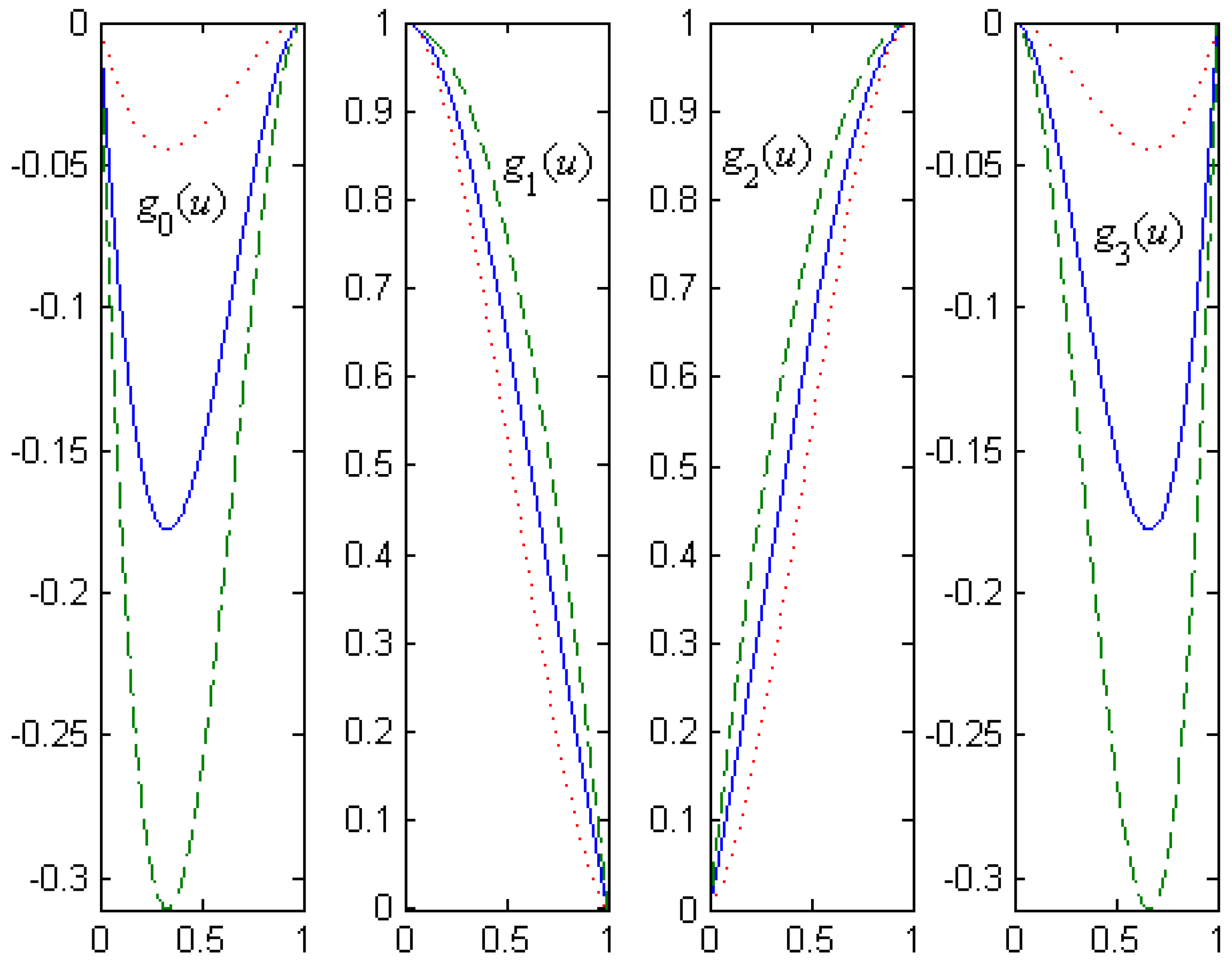
Theorem 1 shows that the cubic
α-Catmull-Rom basis functions not only inherit the properties of the standard cubic Catmull-Rom basis functions, but also can be adjusted by the shape parameter
α.
Figure 1 shows curves of the cubic
α-Catmull-Rom basis functions for different values of
α, where the value of
α is taken as
(marked with dotted lines),
(marked with solid lines) and
(marked with dashed lines), respectively.
4. The Cubic α-Catmull-Rom Spline Curves
On the basis of the cubic α-Catmull-Rom basis functions, the corresponding cubic Catmull-Rom spline curves with a shape parameter can be defined as follows.
Definition 2. Given control points in or , for , , the following curves are called the cubic Catmull-Rom spline curves with a shape parameter α (cubic α-Catmull-Rom spline curves for short):
where
are the cubic
α-Catmull-Rom basis functions defined in (9).
Theorem 2. The cubic
α-Catmull-Rom spline curves have the following properties:
- (a)
symmetry: for the same shape parameter
α, both
and
define the same curves in a different parameterization:
- (b)
geometric invariance: shapes of the curves are independent of the choice of coordinate system. An affine transformation for the curves can be performed by carrying out the same affine transformation for the control points;
- (c)
local property: at most, four segments of the curves would be affected if one control point is moved;
- (d)
interpolation and C1 continuity: the curves interpolate the given control points expect and , and the curve is C1 continuous;
- (e)
shape adjustable property: when the control points are fixed, shape of the curve can be adjusted by altering the value of the shape parameter α.
Proof. - (a)
From the symmetry of the cubic
α-Catmull-Rom basis functions and Equation (10), then
- (b)
Because Equation (10) is an affine combination of the control points, geometric invariance follows.
- (c)
From Equation (10), a segment of the curve is only related to the four control points , thus, at most, four segments of the curves would be affected if one control point is moved.
- (d)
From the properties at the endpoints of the
α-Catmull-Rom basis functions and Equation (10), then
Equation (11) shows that the curves interpolate the given control points expect
and
. From Equations (11) and (12), it follows that
Equation (13) shows that the curves are C1 continuous.
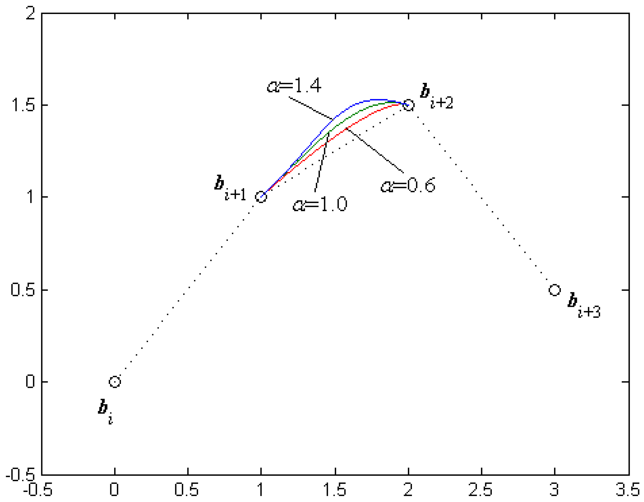
- (e)
Since Equation (10) contains the parameter
α, the shape of the curve
can be adjusted by altering the value of
α even if the control points
are fixed (see
Figure 2).
Theorem 2 shows that the cubic α-Catmull-Rom spline curves not only inherit the same properties of the standard cubic Catmull-Rom spline curves, but also can achieve shape adjustment by the shape parameter α.
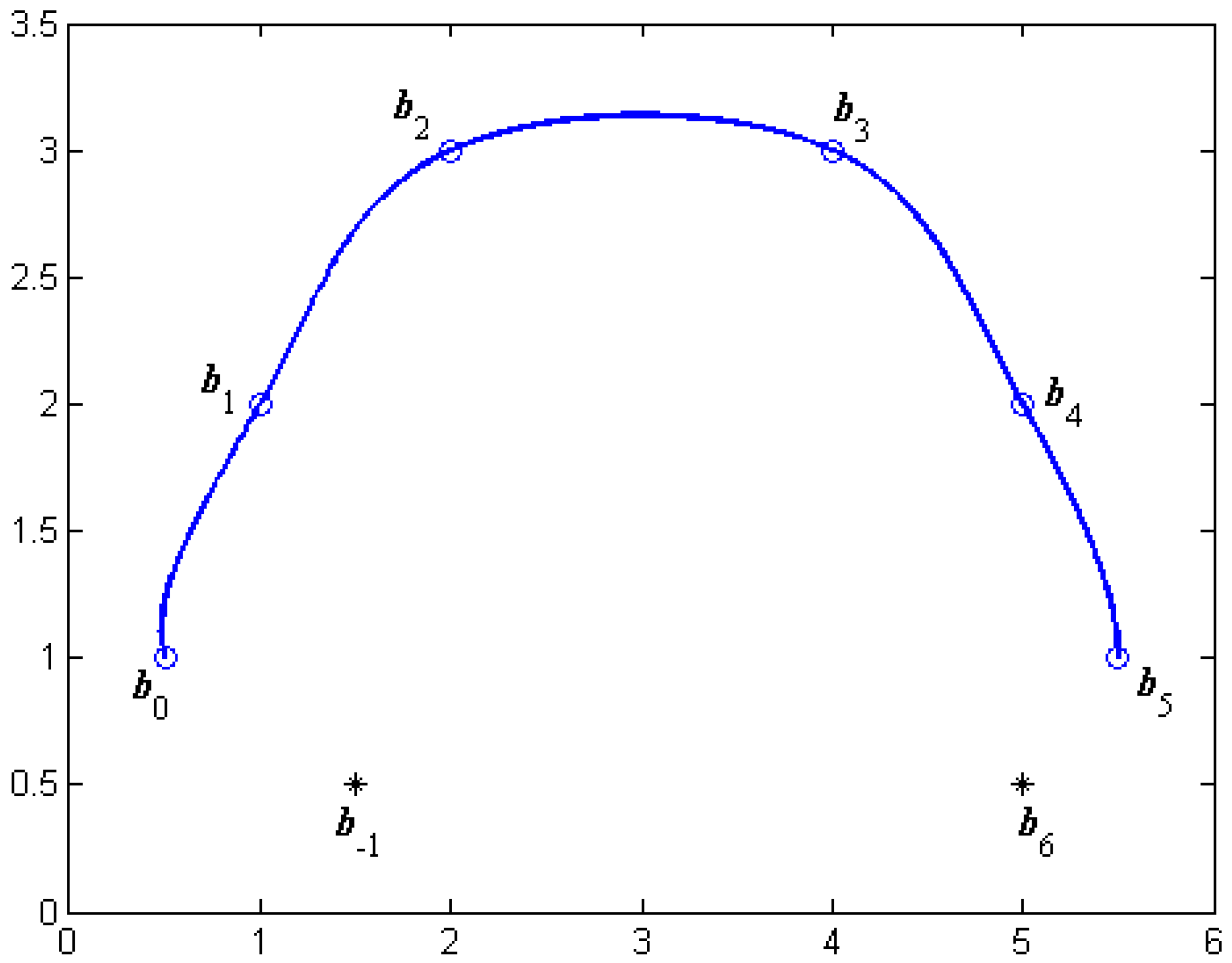
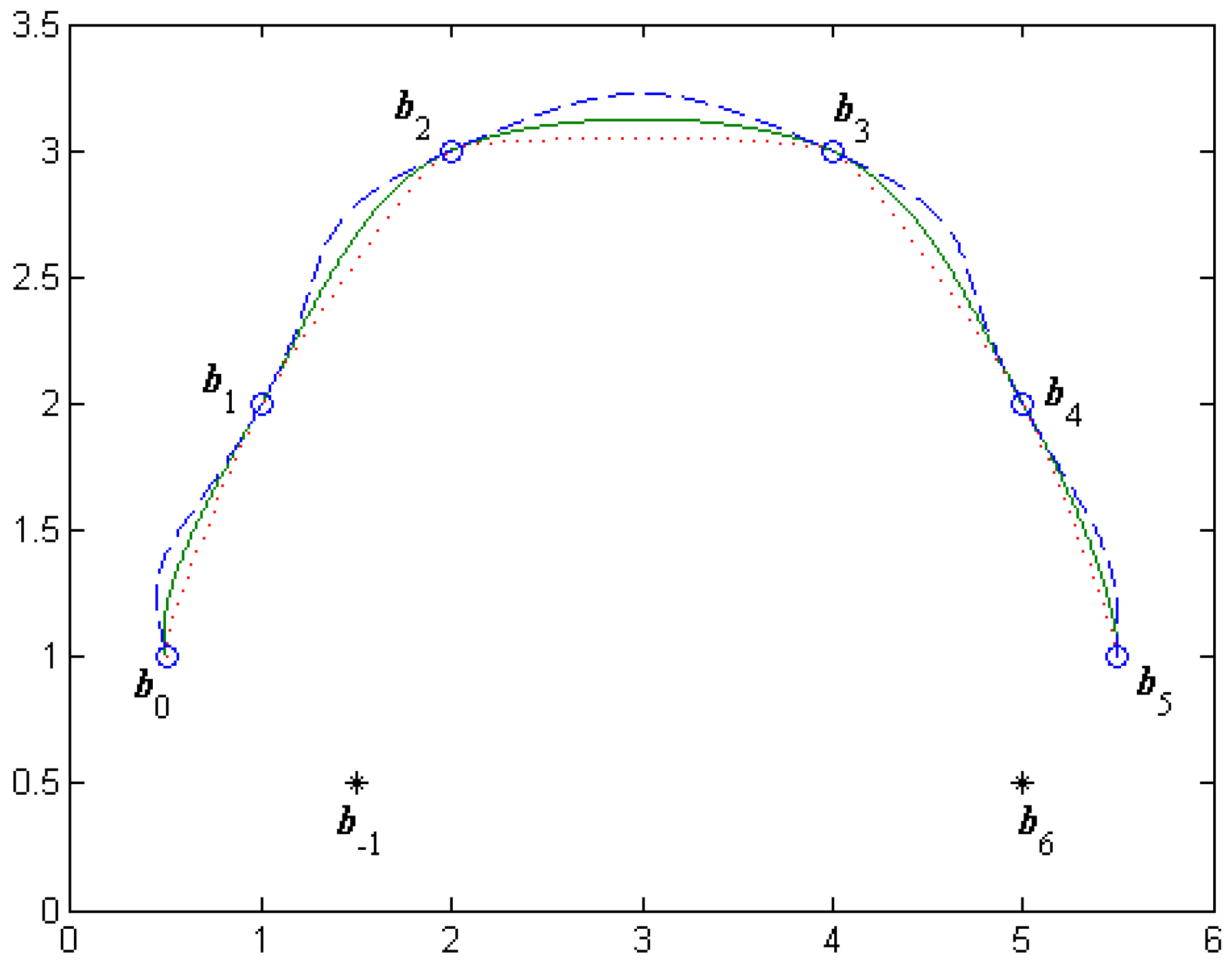
If two auxiliary points
and
are added to the given control points, the
C1 continuous cubic
α-Catmull-Rom spline curves
interpolating all the given control points
would be obtained. It is clear that there exists one degree of freedom in the
C1 continuous cubic
α-Catmull-Rom spline curves, even if the control points and auxiliary points are fixed. Different interpolation curves could be obtained by altering the value of the shape parameter
α.
Figure 3 shows the
C1 continuous cubic
α-Catmull-Rom spline curves adjusted by the shape parameter
α, where the value of
α is taken as
(marked with dotted lines),
(marked with solid lines) and
(marked with dashed lines), respectively.
Remark 2. As we know, the cubic Hermite spline curves [
27] can be expressed as follows:
where
If we let
,
, then Equation (14) could be rewritten as follows:
where
Although the curves expressed in Equation (15) have the similar properties of the proposed α-Catmull-Rom spline curves, the proposed α-Catmull-Rom spline curves are constructed by extending the definition interval of the standard cubic Catmull-Rom spline from [0,1] to [0,α], which is a new idea for constructing cubic Catmull-Rom spline with a shape parameter. Thus, the proposed work provides another method for constructing interpolation curves without solving equation systems.
Since the shapes of the cubic α-Catmull-Rom spline curves are determined by the value of the shape parameter α when the control points and auxiliary points are fixed, how to determine the optimal value of α for making the cubic α-Catmull-Rom spline curves be the smoothest, therefore, needs to be discussed. A method for determining the optimal value of α is presented as follows.
According to Ref. [
28], the smoothness of a parametric curve
can be approximately measured by its energy expressed as follows:
The lower the energy is, the smoother the curve.
From Equation (16), for given data points
and two auxiliary points
,
, the optimal value of
α of the cubic
α-Catmull-Rom spline curves
can be determined by an optimization model expressed as follows:
Then, Equation (10) can be rewritten as follows:
where
,
.
From Equations (17) and (18) can be expressed as follows:
where
,
,
.
Since there is always , the solution of Equation (19) has the following two cases:
Case 1. When . If , the solution of Equation (19) is ; else if , the solution of Equation (19) is ; else, the solution of Equation (19) is α to take any non-negative real number.
Case 2. When . If , the solution of Equation (19) is ; else, the solution of Equation (19) is .
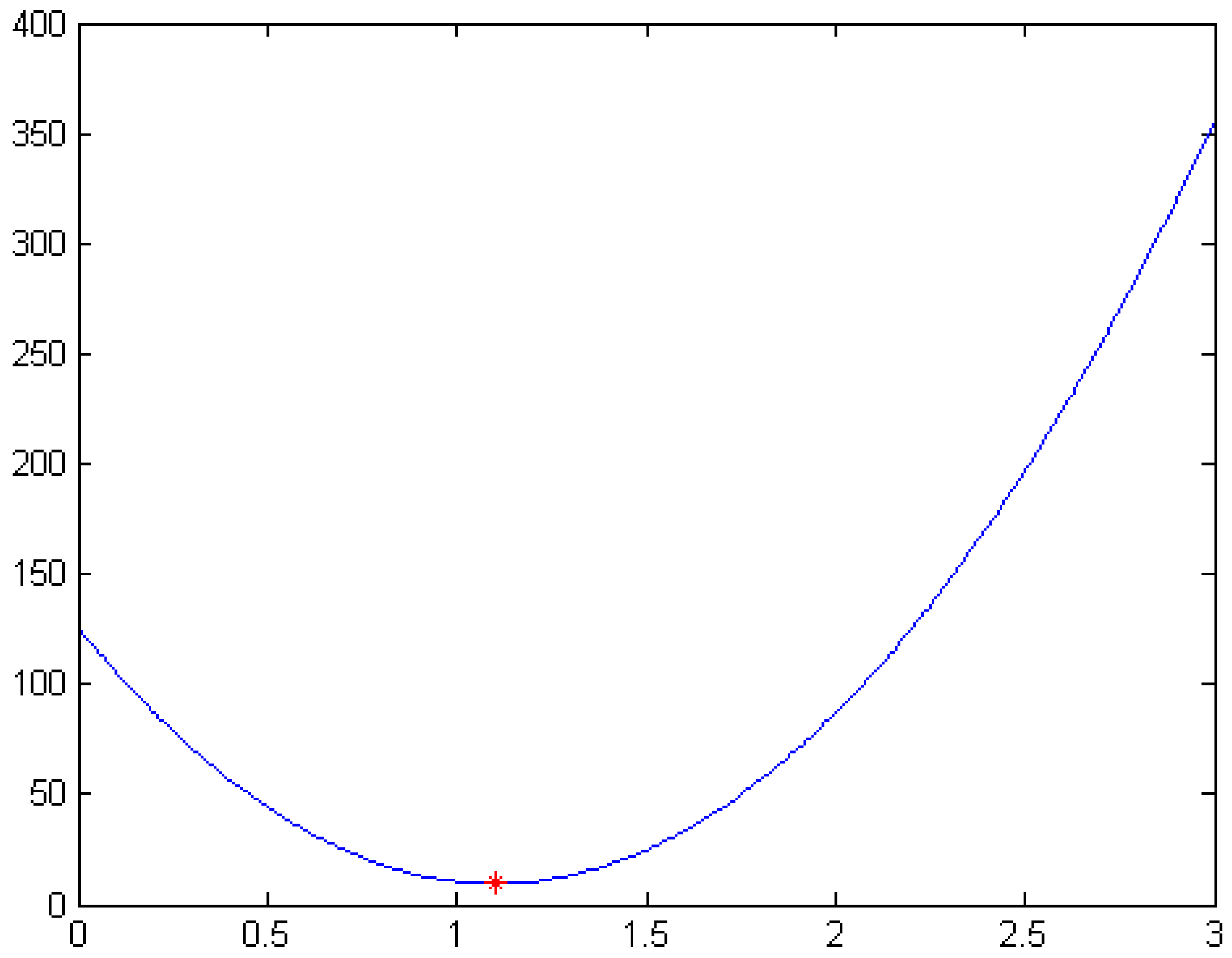
After the optimal value of
α is determined by Equation (19), the smoothest cubic
α-Catmull-Rom spline curves can be obtained. For example, for the same control points and auxiliary points in
Figure 3, the optimal value of
α determined by Equation (19) is
. The energy curve of the cubic
α-Catmull-Rom spline curves for
is shown in
Figure 4. The smoothest cubic
α-Catmull-Rom spline curves are shown in
Figure 5.
5. The Cubic α-Catmull-Rom Spline Interpolation Function
On the basis of the cubic α-Catmull-Rom basis functions, the cubic α-Catmull-Rom spline interpolation function can also be defined as follows.
Definition 3. Given a function
,
is a division of
,
, set
, for
, the function,
is called the cubic Catmull-Rom spline functions with a shape parameter
α (cubic
α-Catmull-Rom spline interpolation function for short), where
are the cubic
α-Catmull-Rom basis functions defined according to Equation (9).
From Theorem 2, the cubic
α-Catmull-Rom spline interpolation function has the properties as follows:
- (a)
interpolation: the cubic
α-Catmull-Rom spline interpolation function interpolate the given data points expect
and
,
- (b)
C1 continuity: the cubic
α-Catmull-Rom spline interpolation function is
C1 continuous, viz.,
- (c)
shape adjustable property: if two auxiliary data points and are added to the given data points, the C1 continuous cubic α-Catmull-Rom spline interpolation function interpolating all the given data points would be obtained. The shape of the curve of the cubic α-Catmull-Rom spline interpolation function can be adjusted by altering the value of the shape parameter α.
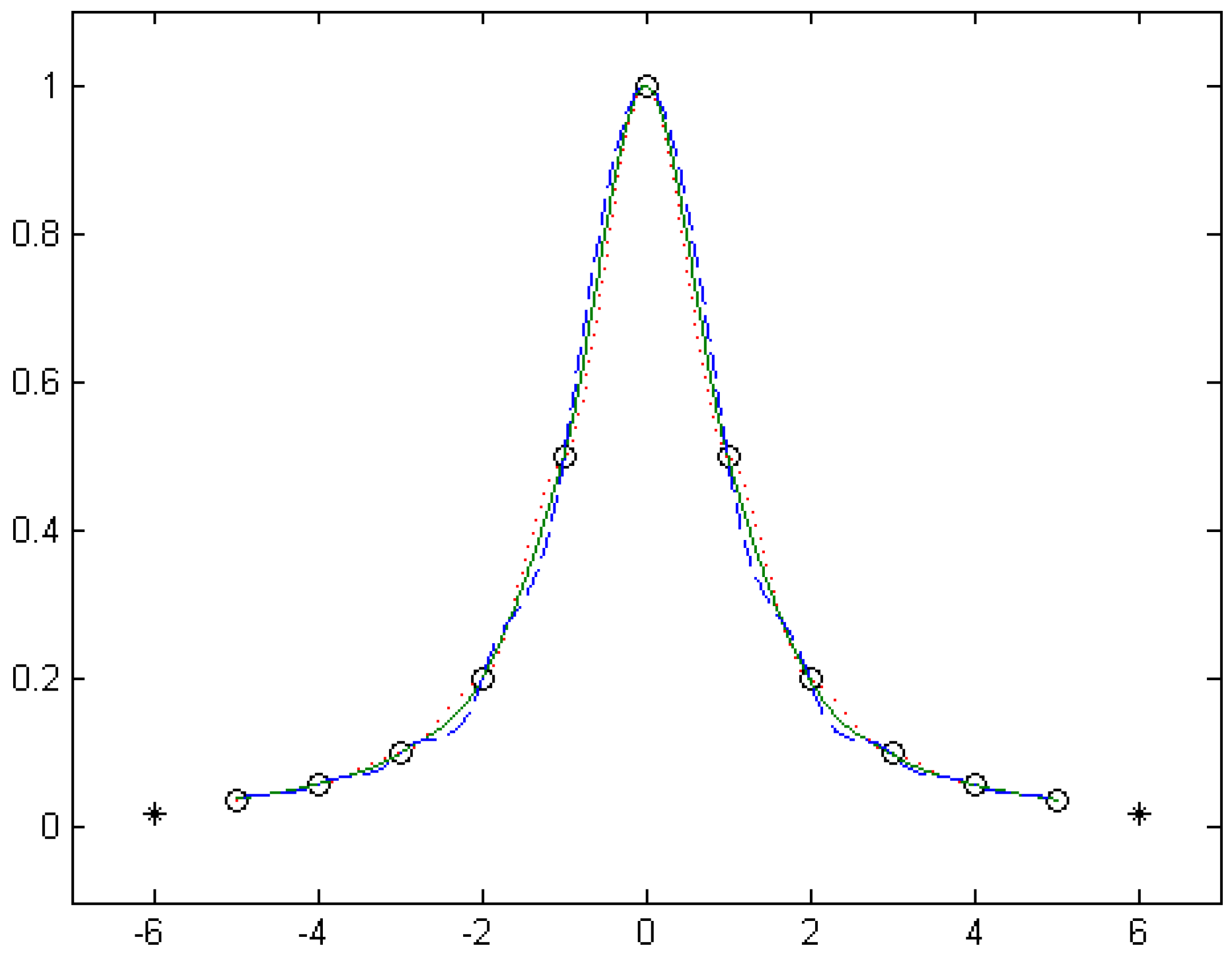
Example 1. Given the function,
set
,
. The two auxiliary data points are taken as follows:
Figure 6 shows the curve of the
C1 continuous cubic
α-Catmull-Rom spline interpolation function adjusted by the shape parameter
α, where the value of
α is taken as
(marked with dotted lines),
(marked with solid lines) and
(marked with dashed lines), respectively.
It is clear that the cubic α-Catmull-Rom spline interpolation function is completely determined by the shape parameter α when the data points and two auxiliary data points are fixed. Hence, how to determine the optimal value of the shape parameter α is the key when constructing the cubic α-Catmull-Rom spline interpolation function. A method for determining the optimal value of the shape parameter α is presented as follows.
Given a function
,
is a division of
,
, and two auxiliary data points
,
are added to the given data points. Then, the interpolation error of the cubic
α-Catmull-Rom spline interpolation function
can be expressed as follows:
where
.
In order to obtain the minimum interpolation error, the following optimal model can be obtained:
Let
, and set
Then, Equation (20) can be rewritten as follows:
where
,
.
From Equations (22) and (23) can be expressed as follows:
where
,
,
.
Since there is always , the solution of Equation (24) has the following two cases:
Case 1. When . If , the solution of Equation (24) is ; else if , the solution of Equation (24) is ; else, the solution of Equation (24) is α to take any non-negative real number.
Case 2. When . If , the solution of Equation (24) is ; else, the solution of Equation (24) is .
After the optimal value of the shape parameter α is determined by Equation (24), the optimum cubic α-Catmull-Rom spline interpolation function could be naturally obtained from Equation (20).
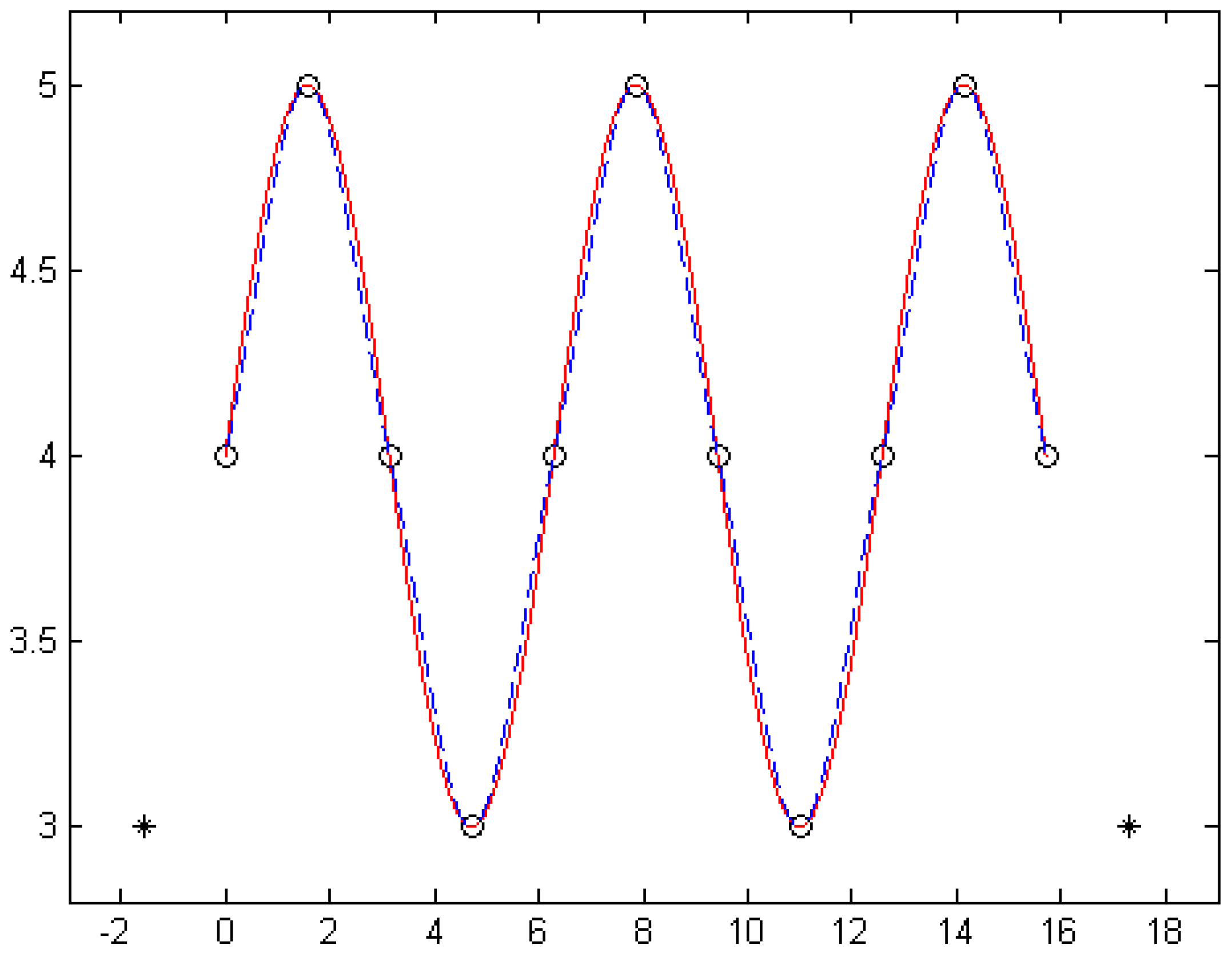
Example 2. Given the function
set
,
. The two auxiliary data points are taken as follows:
For different
n (where
n + 1 is the number of the given data points), the optimal value of the shape parameter
α solved by Equation (24), the interpolation errors of the optimum cubic
α-Catmull-Rom spline interpolation function and the interpolation error of the standard cubic Catmull-Rom spline interpolation function calculated by Equation (21) are shown in
Table 1.
Table 1 shows that the interpolation result of the optimum cubic
α-Catmull-Rom spline interpolation function is better than the standard cubic Catmull-Rom spline interpolation function, which is due to the fact that the shape parameter
α is taken as the optimal value.
The curves of the optimum cubic
α-Catmull-Rom spline interpolation function for
n = 10 (marked with solid lines) and the standard cubic Catmull-Rom spline interpolation function (i.e., the shape parameter is taken as
, marked with dashed lines) are shown in
Figure 7.
6. Conclusions
A cubic α-Catmull-Rom spline with a shape parameter is presented in this paper. The spline curves not only have the same properties as the standard cubic Catmull-Rom spline curves, but can also achieve shape adjustment by altering the value of the shape parameter, even if the control points are fixed. The corresponding cubic α-Catmull-Rom spline interpolation function has the same characteristics with the spline curves, and the optimal interpolation function can be obtained by choosing proper values of the shape parameter. The examples illustrate the feasibility of those methods.
Furthermore, the corresponding spline surfaces and binary interpolation function with shape parameters could be constructed by using tensor products. The spline surfaces and binary interpolation functions would enjoy the same characteristics with the one-dimensional models. Some results in this area will be presented in the following study.


