A Two-Step Global Alignment Method for Feature-Based Image Mosaicing

Abstract

Image mosaicing sits at the core of many optical mapping applications with mobile robotic platforms. As these platforms have been evolving rapidly and increasing their capabilities, the amount of data they are able to collect is increasing drastically. For this reason, the necessity for efficient methods to handle and process such big data has been rising from different scientific fields, where the optical data provides valuable information. One of the challenging steps of image mosaicing is finding the best image-to-map (or mosaic) motion (represented as a planar transformation) for each image while considering the constraints imposed by inter-image motions. This problem is referred to as Global Alignment (GA) or Global Registration, which usually requires a non-linear minimization. In this paper, following the aforementioned motivations, we propose a two-step global alignment method to obtain globally coherent mosaics with less computational cost and time. It firstly tries to estimate the scale and rotation parameters and then the translation parameters. Although it requires a non-linear minimization, Jacobians are simple to compute and do not contain the positions of correspondences. This allows for saving computational cost and time. It can be also used as a fast way to obtain an initial estimate for further usage in the Symmetric Transfer Error Minimization (STEMin) approach. We presented experimental and comparative results on different datasets obtained by robotic platforms for mapping purposes.

1. Introduction

Rapid progress in technology makes it possible to obtain and store a vast amount of optical data even from areas beyond human reach. The data has been used for several different purposes in the computer vision field. Image mosaicing is one of the common computer vision tools being mainly used for optical mapping and panorama creation. Image mosaicing can be defined as a process of creating a single high-resolution image from overlapping relatively low-resolution images [1], and it has been successfully used for different applications, such as video stabilization [2], mapping both aerial [3] and underwater [4], panorama creation [5,6,7], and super-resolution [8], among others. Image mosaicing is composed of two main steps, namely registration and blending. The registration step is further divided into two steps: pairwise and global registration (or GA). Pairwise registration (or image matching) consists of finding a relative motion (or transformation) between the coordinate frames of two overlapping images, while Global Alignment (GA) aims at finding the motion between image and map (or mosaic) coordinate frame. Intensity blending is applied after aligning images geometrically on mosaic frame in order to reduce the photometric inconsistences between images.

The overall image registration framework starts by detecting some salient points in the images referred to as features. Then, features are described with a vector obtained via different image gradient information. Similar descriptors are matched between images by using a distance metric (generally Euclidean distance). Due to noise, some of the descriptors might not be matched correctly. They are called Outliers, and they need to be eliminated. To do so, usually robust estimation algorithms (such as Random Sample Consensus (RANSAC) [9]) are employed. Once the outliers are removed, consistent registration parameters (transformation or motion) between images can be estimated [10] and referred to as relative transformation. Once the pairwise image registration (both time-consecutive and non-time-consecutive) is completed, a list of overlapping image pairs and relative registration parameters between them become available. The next step in the Feature-based Image Mosaicing (FIM) framework is GA to obtain mosaics. GA is the problem of finding the image-to-mosaic registration parameters that comply best with constraints imposed by all overlapping image pairs. Global projection of images (global or absolute transformation) can be calculated by successively multiplying relative transformations between time-consecutive images if one of the image frames is selected as a global frame. Usually, the first image frame is chosen as a global frame if there is no other relevant information available. Since relative transformations encapsulate some errors due to the positions of correspondences and the estimation methods, accumulation of errors yields a bigger error and results in the form of misalignment and distortions on image size. GA methods are needed to overcome this error accumulation. As GA is one of important steps in the image mosaicing pipeline, there have been several methods proposed. One of the classifications can be done according to in which domain the error is minimized, mosaic or image. The minimization on the mosaic frame has as a drawback the tendency to reduce the size of the mosaiced images, as reducing the size also decreases the error. However, this way of minimization can be done linearly up to affine motion model. While the errors defined on image frame do not suffer this scaling problem, the minimization usually requires a non-linear minimization. Sawhney et al. [11] proposed minimizing the distances between correspondences on the mosaic frame with an additional error term on the diagonals of images in order to overcome scaling problem. However, having constraints on the image size can cause some disturbance on image alignment. Capel [8] formulated the GA problem similarly to BA [12] approaches in 3D. Point positions on the mosaic frame and absolute transformations are considered as unknowns. This method requires feature tracking and high-overlapping image pairs in order to have certain amount of tracked features on each image. There are also GA methods [13,14] that apply image-to-mosaic registration, known as “online mosaicing”. In such cases, if there appears a failure while mapping one image onto the mosaic, future image-to-mosaic registration is likely to fail. Generally, errors (Euclidean distance between where the relative planar transformation maps a point and the correspondence of the point was originally detected. An illustration can be seen in Figure 1) defined on image frame have been preferred and widely used. However, non-linear minimization can be still regarded as a bottleneck for large-scale mapping applications due to the computational cost and prerequisite of good initial estimate. In this paper, we propose a two-step GA method aimed to be fast and less computationally demanding. The first step is to estimate scale and rotation parameters, while the second step is for estimating translational parameters. We also show that our proposal can be used in order to find an accurate initial estimate for gold-standard GA methods.

2. Nomenclature

• n is the total number of images.
• $c_{ij}$ is the total number of correspondences between images i and j.
• $s,\mathsf{\theta },t^x,\mathrm{andd}{t}^y$ represents the scale, rotation (in radians) and translation parameters (in pixels) of a similarity type planar transformation

  $$\begin{array}{ccc}\hfill \mathbf{H}& =& \left[\begin{array}{ccc}s·cos\mathsf{\theta }& -s·sin\mathsf{\theta }& t^x\\ s·sin\mathsf{\theta }& s·cos\mathsf{\theta }& t^y\\ 0& 0& 1\end{array}\right]\hfill \end{array}$$
• ${}^i\mathbf{H}_j$ is the transformation relating image points represented in the coordinate frame image j to the coordinate frame of image i and it consists of parameters (${}^{i}s_j,{}^i\mathsf{\theta }_j,{}^{i}t_j^x,{}^{i}t_j^y$).
• The transformation from image i to the global frame m is represented with ${}^m\mathbf{H}_i$. ${}^m\mathbf{H}_i$ is composed of parameters ($s_i,{\mathsf{\theta }}_i,t_i^x,t_i^y$) similarly above. For simplicity, m is dropped in the representation of parameters.
• The first image frame is selected as a mosaic frame. Therefore, ${}^m\mathbf{H}_1$ is identity and m equals to 1. Parameters for the first image are not considered as unknown.

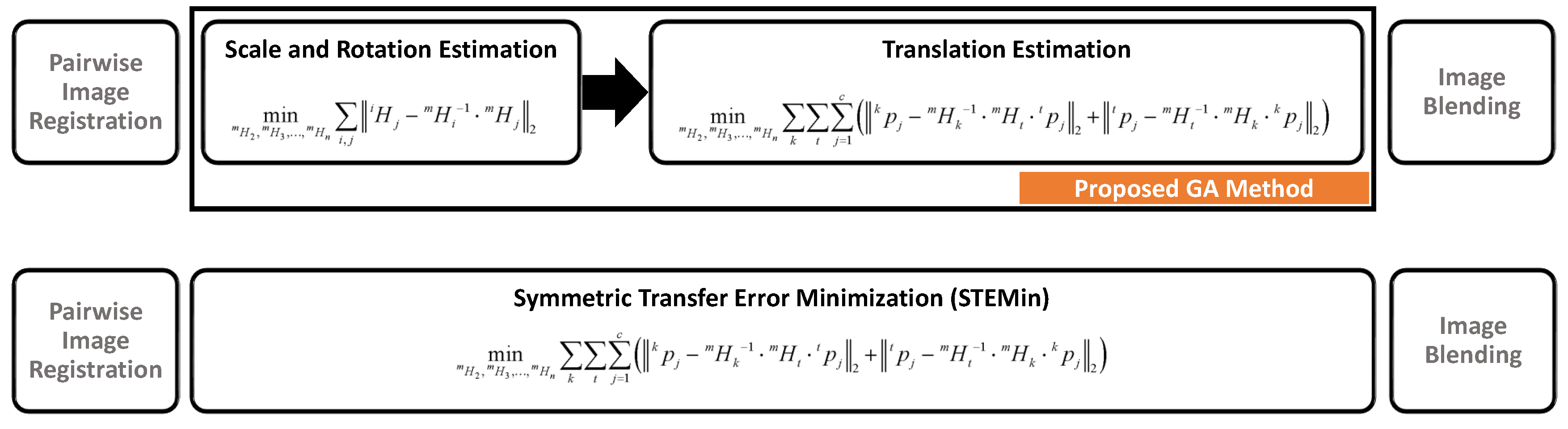
3. Two-Step Global Alignment for Feature-Based Image Mosaicing (FIM)

Our GA approach is motivated by the constraints imposed by relative transformations between overlapping images as absolute transformations should meet the constraints introduced by them. We use similarity type planar transformations as they generally contain enough Degrees of Freedom (DOFs) for optical mapping with robotic platforms [15]. A pipeline of the proposed GA method is illustrated in Figure 2.

3.1. Scale and Rotation Estimation

First, we try to obtain the optimum scale and rotation parameters for each image by minimizing the error given in Equation (1) over scale and rotation without taking into account the translation parameters:

$$\begin{array}{cc}\underset{{}^m\mathbf{H}_1,{}^m\mathbf{H}_2,{}^m\mathbf{H}_3\dots {}^m\mathbf{H}_n}{min}{\displaystyle \sum _{i,j}}\hfill & \parallel {}^i\mathbf{H}_j-{}^m\mathbf{H}_i^{-1}·{}^m\mathbf{H}_j{\parallel }_2\hfill \end{array}$$

(1)

where i and j are the indices of the images that were successfully matched overlapping image pairs. Without taking into translation parts, Equation (1) can be rewritten as follows:

$$\begin{array}{ccc}{E}_1(s_{2,\dots ,n},{\mathsf{\theta }}_{2,\dots ,n})\hfill & =\hfill & {\displaystyle \sum _{i,j}}\parallel {}^{i}s_j-\frac{s_j}{s_i}{\parallel }_2+\parallel {}^i\mathsf{\theta }_j-({\mathsf{\theta }}_j-{\mathsf{\theta }}_i){\parallel }_2\hfill \end{array}$$

(2)

It should be noted that the $E_1$ is written as sum of errors in scale and rotation. As there is no dependency between parameters, minimization can be applied separately:

$$\begin{array}{ccc}{E}_{11}(s_2,\dots ,s_n)\hfill & =\hfill & {\displaystyle \sum _{i,j}}\parallel {}^{i}s_j-\frac{s_j}{s_i}{\parallel }_2\hfill \\ & =\hfill & {\displaystyle \sum _{i,j}}{\mathit{r}}_{1\mathit{i}\mathit{j}}^T·{\mathit{r}}_{1\mathit{i}\mathit{j}}\hfill \\ E_{12}({\mathsf{\theta }}_2,\dots ,{\mathsf{\theta }}_n)\hfill & =\hfill & {\displaystyle \sum _{i,j}}\parallel {}^i\mathsf{\theta }_j-({\mathsf{\theta }}_j-{\mathsf{\theta }}_i){\parallel }_2\hfill \\ & =\hfill & {\displaystyle \sum _{i,j}}{\mathit{r}}_{2\mathit{i}\mathit{j}}^T·{\mathit{r}}_{2\mathit{i}\mathit{j}}\hfill \end{array}$$

(3)

where ${\mathit{r}}_{1\mathit{i}\mathit{j}}=\left[\begin{array}{c}{}^{i}s_j-\frac{s_j}{s_i}\end{array}\right]$ and $E_{12}$ can be minimized linearly as similarly done in [16]. Operating on Euler angles may suffer from singularities; therefore, we apply non-linear minimization using trigonometric functions coming from the equation ${}^i\mathbf{R}_j-{{\mathbf{R}}^{-1}}_i·{\mathbf{R}}_j$, where $\mathbf{R}$ represents the two-dimensional rotation matrix. For non-linear minimization, the residual vector is written of as follows:

$${\mathit{r}}_{2\mathit{i}\mathit{j}}=\left[\begin{array}{c}cos\left({}^i\theta _j\right)-cos({\mathsf{\theta }}_i-{\mathsf{\theta }}_j)\\ sin\left({}^i\theta _j\right)+sin({\mathsf{\theta }}_i-{\mathsf{\theta }}_j)\end{array}\right]$$

Jacobians of the cost functions $E_{11}$ and $E_{12}$ are rather simple and can be calculated in block form using the following structural elements:

$$\frac{\partial {\mathit{r}}_{1\mathit{i}\mathit{j}}}{\partial s_i}=\left[\begin{array}{c}\frac{\mathrm{sj}}{{\mathrm{si}}^2}\end{array}\right],\frac{\partial {\mathit{r}}_{1\mathit{i}\mathit{j}}}{\partial s_j}=\left[\begin{array}{c}-\frac{1}{{\mathrm{s}}_{\mathrm{i}}}\end{array}\right],$$

$$\frac{\partial {\mathit{r}}_{2\mathit{i}\mathit{j}}}{\partial {\mathsf{\theta }}_i}=\left[\begin{array}{c}sin({\mathsf{\theta }}_i-{\mathsf{\theta }}_j)\\ cos({\theta }_i-{\mathsf{\theta }}_j)\end{array}\right],and\frac{\partial {\mathit{r}}_{2\mathit{i}\mathit{j}}}{\partial {\theta }_j}=\left[\begin{array}{c}-sin({\mathsf{\theta }}_i-{\mathsf{\theta }}_j)\\ -cos({\mathsf{\theta }}_i-{\mathsf{\theta }}_j)\end{array}\right].$$

As it can be noted, the following relation between Jacobians hold:

$$\frac{\partial {\mathit{r}}_{2\mathit{i}\mathit{j}}}{\partial {\mathsf{\theta }}_i}=-\frac{\partial {\mathit{r}}_{2\mathit{i}\mathit{j}}}{\partial {\mathsf{\theta }}_j}$$

This allows for fast computation for the Jacobian blocks.

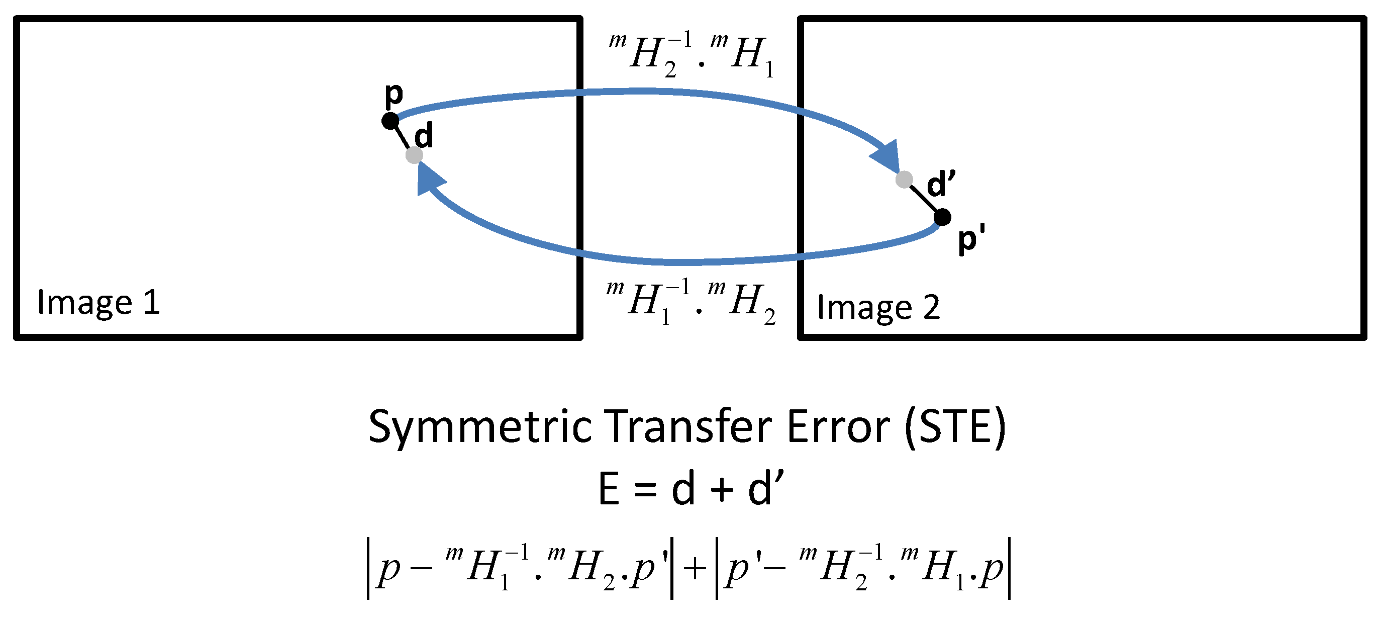
3.2. Translation Estimation

After estimating the scale and rotation parameters by minimizing the error term $E_1=E_{11}+E_{12}$, we minimize STE given in Equation (4) over only translation parameters by using the obtained scale and angle parameters:

$$\begin{array}{c}{E}_2(t_{2,\dots ,n}^x,t_{2,\dots ,n}^y)={\displaystyle \sum _{i,j}}{\displaystyle \sum _{k=1}^c}\left(\parallel {}^{i}p_k-{}^m\mathbf{H}_i^{-1}·{}^m\mathbf{H}_j·{}^{j}p_k{\parallel }_2+\parallel {}^{j}p_k-{}^m\mathbf{H}_j^{-1}·{}^m\mathbf{H}_i·{}^{i}p_k{\parallel }_2\right)\\ \multicolumn{1}{c}{\underset{{t^x}_2,{t^y}_2,\dots ,{t^x}_n,{t^y}_n}{min}{\displaystyle \sum _{i,j}}{\displaystyle \sum _k}{\mathit{t}}_{\mathit{i}\mathit{j}}^T\left(k\right)·{\mathit{t}}_{\mathit{i}\mathit{j}}\left(k\right)}\end{array}$$

(4)

where

$${\mathit{t}}_{\mathit{i}\mathit{j}}\left(k\right)=\left[\begin{array}{c}{}^{i}x_k-\left(a_{ij}·{}^{j}x_k-b_{ij}·{}^{j}y_k+\left(\frac{(t_j^x-t_i^x)·cos{\mathsf{\theta }}_i+(t_j^y-t_i^y)·sin{\mathsf{\theta }}_i}{s_i}\right)\right)\\ {}^{i}y_k-\left(b_{ij}·{}^{j}x_k+a_{ij}·{}^{j}y_k+\left(\frac{(t_j^y-t_i^y)·cos{\mathsf{\theta }}_i+(t_j^x-t_i^x)·sin{\mathsf{\theta }}_i}{s_i}\right)\right)\\ {}^{j}x_k-\left(a_{ji}·{}^{i}x_k-b_{ji}·{}^{i}y_k+\left(\frac{(t_i^x-t_j^x)·cos{\mathsf{\theta }}_j+(t_i^y-t_j^y)·sin{\mathsf{\theta }}_j}{s_j}\right)\right)\\ {}^{j}y_k-\left(b_{ji}·{}^{i}x_k+a_{ji}·{}^{i}y_k+\left(\frac{(t_i^y-t_j^y)·cos{\mathsf{\theta }}_j+(t_i^x-t_j^x)·sin{\mathsf{\theta }}_j}{s_j}\right)\right)\end{array}\right].$$

${}^{j}p_k=({}^{j}x_k,{}^{j}y_k,1)$ and ${}^{i}p_k=({}^{i}x_k,{}^{i}y_k,1)$ are the corresponding feature points in overlapping images i and j. Coefficients a and b are as follows: $a_{ij}=(s_j/s_i)·cos({\mathsf{\theta }}_j-{\mathsf{\theta }}_i)$, $b_{ij}=(s_j/s_i)·sin({\mathsf{\theta }}_j-{\mathsf{\theta }}_i),a_{ji}=(s_i/s_j)·cos({\mathsf{\theta }}_i-{\mathsf{\theta }}_j)$, and $b_{ji}=(s_i/s_j)·sin({\mathsf{\theta }}_i-{\mathsf{\theta }}_j)$. As the error term $E_2$ is minimized over translation parameters, its Jacobian matrices are also easy to compute:

$$\frac{\partial {\mathit{t}}_{\mathit{i}\mathit{j}}\left(k\right)}{\partial \left(t_i^x\right)}={\left[\begin{array}{cccc}\frac{cos{\mathsf{\theta }}_{\mathrm{i}}}{{\mathrm{s}}_{\mathrm{i}}}& \frac{sin{\mathsf{\theta }}_{\mathrm{i}}}{{\mathrm{s}}_{\mathrm{i}}}& -\frac{cos{\mathsf{\theta }}_{\mathrm{j}}}{{\mathrm{s}}_{\mathrm{j}}}& -\frac{sin{\mathsf{\theta }}_{\mathrm{j}}}{{\mathrm{s}}_{\mathrm{j}}}\end{array}\right]}^T,$$

$$\frac{\partial {\mathit{t}}_{\mathit{i}\mathit{j}}\left(k\right)}{\partial \left(t_i^y\right)}={\left[\begin{array}{cccc}\frac{sin{\mathsf{\theta }}_{\mathrm{i}}}{{\mathrm{s}}_{\mathrm{i}}}& \frac{cos{\mathsf{\theta }}_{\mathrm{i}}}{{\mathrm{s}}_{\mathrm{i}}}& -\frac{sin{\mathsf{\theta }}_{\mathrm{j}}}{{\mathrm{s}}_{\mathrm{j}}}& -\frac{cos{\mathsf{\theta }}_{\mathrm{j}}}{{\mathrm{s}}_{\mathrm{j}}}\end{array}\right]}^T,$$

$$\frac{\partial {\mathit{t}}_{\mathit{i}\mathit{j}}\left(k\right)}{\partial \left(t_j^x\right)}={\left[\begin{array}{cccc}-\frac{cos{\mathsf{\theta }}_{\mathrm{i}}}{{\mathrm{s}}_{\mathrm{i}}}& -\frac{sin{\mathsf{\theta }}_{\mathrm{i}}}{{\mathrm{s}}_{\mathrm{i}}}& \frac{cos{\mathsf{\theta }}_{\mathrm{j}}}{{\mathrm{s}}_{\mathrm{j}}}& \frac{sin{\mathsf{\theta }}_{\mathrm{j}}}{{\mathrm{s}}_{\mathrm{j}}}\end{array}\right]}^T$$

,and

$$\frac{\partial {\mathit{t}}_{\mathit{i}\mathit{j}}\left(k\right)}{\partial \left(t_j^y\right)}={\left[\begin{array}{cccc}-\frac{sin{\mathsf{\theta }}_{\mathrm{i}}}{{\mathrm{s}}_{\mathrm{i}}}& -\frac{cos{\mathsf{\theta }}_{\mathrm{i}}}{{\mathrm{s}}_{\mathrm{i}}}& \frac{sin{\mathsf{\theta }}_{\mathrm{j}}}{{\mathrm{s}}_{\mathrm{j}}}& \frac{cos{\mathsf{\theta }}_{\mathrm{j}}}{{\mathrm{s}}_{\mathrm{j}}}\end{array}\right]}^T.$$

The following relation between Jacobians can be seen easily.

$$\frac{\partial {\mathit{t}}_{\mathit{i}\mathit{j}}\left(k\right)}{\partial \left(t_j^x\right)}=-\frac{\partial {\mathit{t}}_{\mathit{i}\mathit{j}}\left(k\right)}{\partial \left(t_i^x\right)}and\frac{\partial {\mathit{t}}_{\mathit{i}\mathit{j}}\left(k\right)}{\partial \left(t_j^y\right)}=-\frac{\partial {\mathit{t}}_{\mathit{i}\mathit{j}}\left(k\right)}{\partial \left(t_i^y\right)}.$$

This relation further reduces the computational cost of Jacobian computation. It can also be noted that Jacobian matrices are free of any feature point positions. This allows Jacobian matrices to be computed fast.

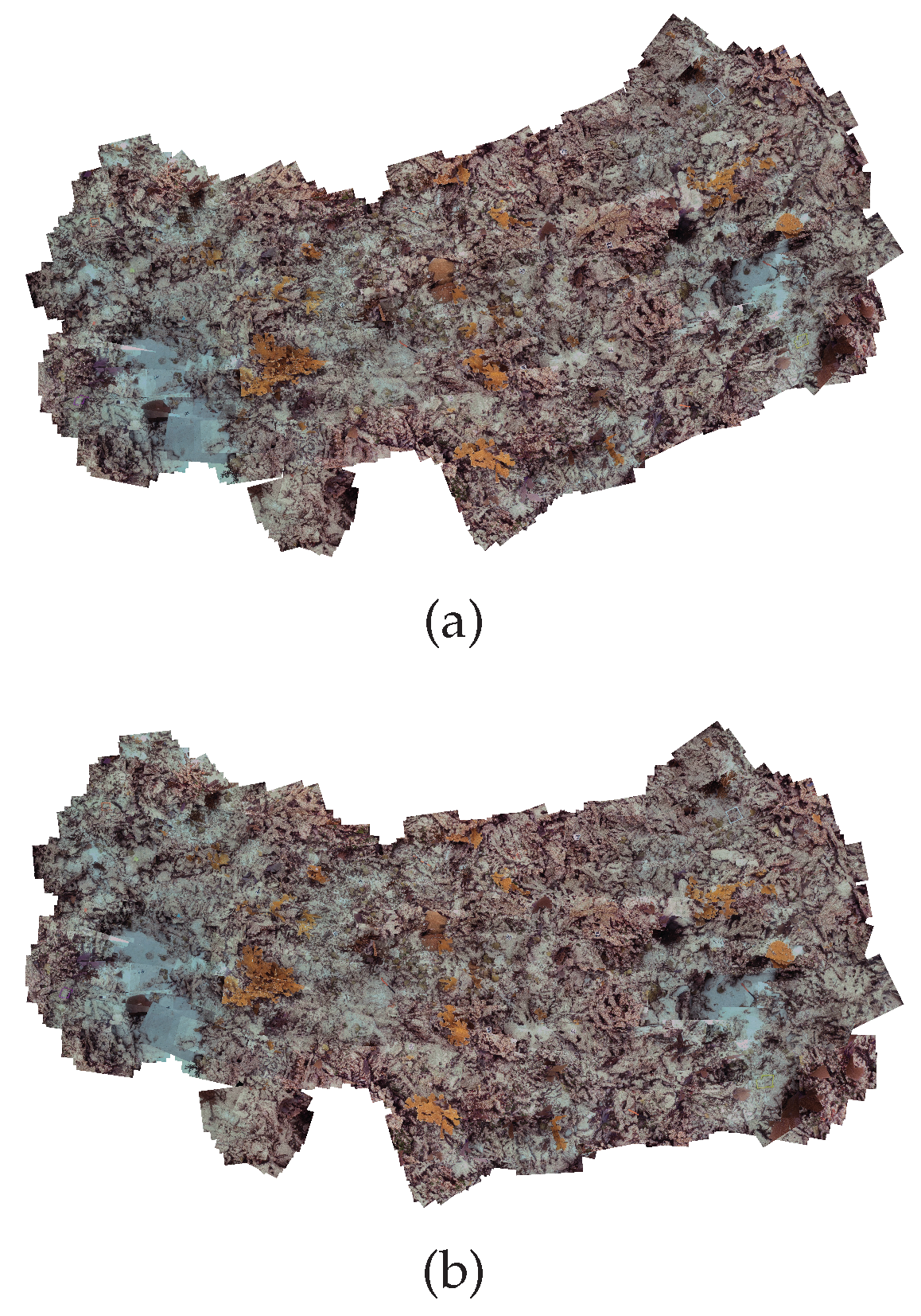
4. Experimental Results

We have tested our proposal on several datasets obtained by different underwater robotic platforms. Main characteristics of the datasets are summarized in

Table 1. Properties of datasets used in experiments.

Dataset	Image Size	Color	Total Number of			Scale		Angle in Degree		Overlapping Area 1 (in Percent)
			Images	Overlapping Pairs	Correspondences	min.	max.	min.	max.	min.	mean	max.
Dataset I	$512\times 384$	RGB	486	3225	360,262	0.73	1.33	-45.07	52.51	15.91	64.28	97.65
Dataset II	$1440\times 806$	RGB	493	3686	259,443	0.62	1.74	-40.33	51.54	13.93	62.03	96.64
Dataset III	$512\times 384$	RGB	1136	3798	550,845	0.76	1.39	-37.55	49.16	18.12	72.98	96.10
Dataset IV	$384\times 288$	Grayscale	430	5412	930,898	0.78	1.26	-31.70	72.31	22.57	64.18	99.04
Dataset V	$1024\times 1024$	RGB	245	3311	2,218,502	0.74	1.44	-0.77	0.78	1.06	38.82	97.35
Dataset VI	$1344\times 752$	RGB	3031	14,132	2,322,233	0.61	1.54	-70.45	66.93	5.02	56.06	96.97
Dataset VII	$384\times 287$	RGB	268	3688	1,425,402	0.85	1.19	-179.84	179.85	6.13	40.98	96.42

${}^1$ The numbers reported in this column are computed over overlapping image pairs given in the fifth column of the table.

. Datasets I, III, and VI were obtained using a Flea digital camera (Point Grey, Vancouver, BC, Canada) carried by a Phantom XTL Remotely Operated Vehicle (ROV) (Deep Ocean Engineering, Inc., San José, CA, USA) during a survey of a patch of reef located in the Florida Reef Tract [18]. Dataset IV was gathered by the $ICTINE{U}^{AUV}$ [17] underwater robot during sea experiments on the Mediterranean coast of Spain. The Dataset VII was acquired by the $Girona{500}^{AUV}$ [19] during its operational tests in the pool of the Underwater Robotics Center at the University of Girona. The floor of the pool was covered by a big poster in order to simulate realistic environment. The robot was equipped with different navigation sensors that provide pose information as rotation and translation in 3D. By combining pose with camera calibration information, planar transformations for each image can be computed. These transformations are 8-DOF full projective type and obtained results are presented as Sensor 8-DOFs in

Table 2. Summary of results. STEMin represents direct minimization of STE. Strategy Combined denotes STEMin using the results of the proposed method as an initial estimate.

Dataset	Strategy	Avg. Error	Std. Deviation	Max. Error	Final Mosaic Size	Time 2
		in Pixels	in Pixels	in Pixels	in Pixels	in Seconds
Dataset I	Proposed method	7.69	3.32	41.22	37432419	13.48
	STEMin	6.08	2.70	36.68	35492284	104.16
	Combined	6.08	2.70	36.68	35492284	73.00
Dataset II	Proposed method	24.72	12.10	181.47	60357134	10.69
	STEMin	20.39	9.93	155.50	59497239	93.45
	Combined	20.39	9.93	155.50	59497239	47.89
Dataset III	Proposed method	6.50	2.64	54.57	36112352	17.93
	STEMin	5.54	2.37	40.50	36232346	141.31
	Combined	5.54	2.37	40.50	36232346	110.77
Dataset IV	Proposed method	6.18	2.76	58.88	31872602	41.96
	STEMin	5.80	2.54	61.20	32952674	292.86
	Combined	5.80	2.54	61.20	32952674	222.86
Dataset V	Proposed method	5.55	2.86	44.14	55468475	75.30
	STEMin	5.23	2.72	51.20	55358442	808.90
	Combined	5.23	2.72	51.20	55358442	352.54
Dataset VI	Proposed method	33.82	15.86	266.94	18,93411,710	158.80
	STEMin	24.78	11.38	223.32	20,46711,343	4590.39
	Combined	24.78	11.38	223.32	20,46711,343	835.39
Dataset VII	Proposed method	2.81	1.06	16.96	22031727	80.09
	STEMin	2.35	0.90	17.13	22011728	2885.82
	Combined	2.35	0.90	17.13	22011728	604.72
	Sensor 4-DOFs	2.85	1.18	23.96	21961721	$N.A.$
	Sensor 8-DOFs	1.56	0.82	21.00	19921589	$N.A.$

${}^2$ The current form of our implementation is not optimized. The reported execution times are included to provide an estimate of the time saving between methods. Further improvements can be achieved using some dedicated tools such as Ceres-Solver [21].

. Furthermore, we registered individual images with respect to the image of the poster and obtained results are presented as Sensor 4-DOFs. Although originally the dataset has 286 images, some of them were discarded due to not having sensor readings and not having sufficient correspondences for successful registration as they were acquired close to the borders. Datasets I, II, V, and VI have some (namely, 6, 15, 5, and 42) time-consecutive images that do not have overlapping areas. This causes accumulation of the motion between time-consecutive images that fails to provide an initial estimate of the trajectory. Range for scale and rotation parameters between overlapping image pairs are also presented along with the characteristics. These values are extracted from the planar transformations, which were computed through image registration process. Angles are computed with atan2 function providing values in $[-\mathsf{\pi }/2,\mathsf{\pi }/2]$. Scale Invariant Feature Transform (SIFT) [20] is employed for feature detection and description while RANSAC is used for outlier rejection and transformation estimation. If there are at least 20 remaining correspondences after outlier rejection, image pairs are counted as successfully matched and included as overlapping image pairs. All the tests were performed using a desktop computer with an Intel Xeon E5-1650^™ $3.5Ghz$ processor (Intel Corporation, Santa Clara, CA, USA) with a 64-bit operating system and running MATLAB^™ on the CPU. Error minimization is carried out using a Levenberg–Marquadt algorithm through lsqnonlin function. We have provided analytic expressions for computing the Jacobian matrix. For comparison, we minimized the STE (Equation (4)) over all parameters for each transformation. STE is also chosen for comparing the results obtained as it is independent of the chosen global frame. Results are summarized in Table 2. The second column shows the tested methods: the proposed method and the standard minimization of STE denoted as STEMin. The third, fourth and fifth columns correspond to the average STE, the standard deviation, and maximum error calculated using all the correspondences over all overlapping image pairs. The last column shows the total time spent for error minimization. For the proposed method, the time column provides the sum of the time spent by both $E_1$ and $E_2$ minimizations. Initial estimates for absolute transformations are provided as identity mappings. They are included as a comparison baseline. We also present the basic statistical measures on absolute differences between scale and rotation parameters estimated by the proposed method and STEMin. Results are summarized in

Table 3. Differences between scale and rotation parameters estimated by the proposed method and STEMin.

Dataset	Scale			Angle (in Degree)
	Mean	Std. Deviation	Maximum	Mean	Std. Deviation	Maximum
Dataset I	0.0604	0.0559	0.2047	1.7991	1.2261	7.5344
Dataset II	0.0260	0.0205	0.1134	3.0023	2.4866	11.5737
Dataset III	0.0148	0.0117	0.0609	1.5241	0.9683	5.8098
Dataset IV	0.0390	0.0348	0.1733	1.8220	1.6750	8.1793
Dataset V	0.0035	0.0028	0.0147	0.0974	0.0745	0.4068
Dataset VI	0.0802	0.0619	0.4038	11.4706	3.6440	23.2907
Dataset VII	0.0067	0.0056	0.0263	0.5214	0.2992	1.2662

. From the results, it can be seen that our proposal was able to obtain similar trajectory accuracy with less computational efforts. This is favorable especially on large datasets and/or mapping applications where computational limits may exist. It should be noted that our proposal also makes use of non-linear minimization, which generally requires a good initial estimate for better and quick convergence. Since our proposal performs relatively fast and requires less computational resources, its result can be also used as an initial estimate for minimizing STE, especially when there is no good initial estimate. From the table, it can be seen that running our proposal and using its result as an initial value for STEMin (combined strategy) provides the same level of accuracy with running minimization directly. It should be also noted that using our proposal accelerates the convergence and this yields reduction of the total computational time. If an initial estimate can be obtained by using some other sensor data (e.g., Global Positioning System (GPS), Doppler Velocity Log (DVL),Ultra Short Base Line (USBL)) and/or through relative transformations, this might improve the final convergence.

Although symmetric transfer error helps to infer accuracy about the trajectory, it does not always represent the visual quality of the final mosaic. We use invariant color histograms [22] as a visual comparison of final mosaics as done in [23]. To compare histograms of two images a and b, we use the same metric in [22] and the computation of differences between their histograms is given in Equation (5):

$$d({\mathbf{h}}^a,{\mathbf{h}}^b)=\frac{{\sum }_c{({\mathbf{h}}_c^a-{\mathbf{h}}_c^b)}^2}{{\sum }_c{\left({\mathbf{h}}_c^b\right)}^2},$$

(5)

where ${\mathbf{h}}_c$ denotes the histogram value for color channel c and computed as follows:

$${\mathbf{h}}_c=\sum _{s,s_c=c}|f_x\left(s\right)g_y\left(s\right)-f_y\left(s\right)g_x\left(s\right)|,$$

(6)

where f and g denote derivatives in two color channels [22].

For each dataset, we rendered mosaics using last-on-top strategy. Invariant histograms of rendered mosaics were computed and differences between them were calculated using the Equation (5). Mosaics obtained with STEMin are used as comparison baseline (i.e., histogram b in Equation (5)). Results are presented in

Table 4. Summary of the invariant histogram comparisons.

Dataset	$d(h^a,h^b)$
Dataset I	0.0223
Dataset II	0.0052
Dataset III	0.0038
Dataset V	0.0025
Dataset VI	0.0910
Dataset VII	0.0027
Sensor 4-DOFs	0.0034
Sensor 8-DOFs	0.0610

. Dataset IV was excluded for this comparison as it was composed of grayscale images. Final mosaics for Dataset IV and Dataset VI are given in Figure 3 and Figure 4.

5. Conclusions

Large-area optical mapping through image mosaicing has been in demand from different science communities. One of the most challenging steps in the Feature-Based Image Mosaicing pipeline is GA, which requires non-linear minimization. In this paper, we present a two-step GA method aimed to be fast and less computationally demanding. The first step is for estimating scale and rotation parameters, while the second step is to obtain optimum translation parameters. We present experimental and comparative results over different challenging datasets obtained with robotic platforms aimed for optical mapping. Our proposal can be used as a standalone GA method and can also be used as a better initial estimate provider to STE minimization for quicker convergence. Our proposal is suitable for typical surveys with robotic platforms. Experiments on seven challenging different underwater datasets have been reported and have showed the efficiency of the proposed approach.

References

1. Szeliski, R. Image alignment and stitching: A tutorial. Found. Trends® Comput. Graph. Vis. 2006, 2, 1–104. [Google Scholar] [CrossRef]
2. Hu, R.; Shi, R.; Shen, I.F.; Chen, W. Video Stabilization Using Scale-Invariant Features. In Proceedings of the 11th International Conference on Information Visualization, Zurich, Switzerland, 4–6 July 2007; pp. 871–877.
3. Turner, D.; Lucieer, A.; Watson, C. An automated technique for generating georectified mosaics from ultra-high resolution unmanned aerial vehicle (UAV) imagery, based on structure from motion (SfM) point clouds. Remote Sens. 2012, 4, 1392–1410. [Google Scholar] [CrossRef]
4. Elibol, A.; Gracias, N.; Garcia, R.; Gleason, A.; Gintert, B.; Lirman, D.; Reid, P.R. Efficient autonomous image mosaicing with applications to coral reef monitoring. In Proceedings of the IROS 2011 Workshop on Robotics for Environmental Monitoring, San Francisco, SA, USA, 30 September 2011.
5. Gledhill, D.; Tian, G.; Taylor, D.; Clarke, D. Panoramic imaging—A review. Comput. Graph. 2003, 27, 435–445. [Google Scholar] [CrossRef]
6. Steedly, D.; Pal, C.; Szeliski, R. Efficiently registering video into panoramic mosaics. In Proceedings of the Tenth IEEE International Conference on Computer Vision, Beijing, China, 17–21 October 2005; Volume 2, pp. 1300–1307.
7. Brown, M.; Lowe, D.G. Automatic Panoramic Image Stitching using Invariant Features. Int. J. Comput. Vis. 2007, 74, 59–73. [Google Scholar] [CrossRef]
8. Capel, D.P. Image Mosaicing and Super-Resolution; Springer Verlag: London, United Kingdom, 2004. [Google Scholar]
9. Fischler, M.A.; Bolles, R.C. Random sample consensus: A paradigm for model fitting with applications to image analysis and automated cartography. Commun. ACM 1981, 24, 381–395. [Google Scholar] [CrossRef]
10. Hartley, R.; Zisserman, A. Multiple View Geometry in Computer Vision, 2nd ed.; Cambridge University Press: Harlow, UK, 2004. [Google Scholar]
11. Sawhney, H.; Hsu, S.; Kumar, R. Robust Video Mosaicing through Topology Inference and Local to Global Alignment. In Proceedings of the European Conference on Computer Vision, Freiburg, Germany, 2–6 June 1998; Volume 2, pp. 103–119.
12. Triggs, B.; McLauchlan, P.F.; Hartley, R.I.; Fitzgibbon, A.W. Bundle adjustmenta modern synthesis. In Vision Algorithms: Theory and Practice; Springer: Corfu, Greece, 1999; pp. 298–372. [Google Scholar]
13. Xu, Z. Consistent image alignment for video mosaicing. Signal Image Video Process. 2013, 7, 129–135. [Google Scholar] [CrossRef]
14. Kekec, T.; Yildirim, A.; Unel, M. A new approach to real-time mosaicing of aerial images. Robot. Auton. Syst. 2014, 62, 1755–1767. [Google Scholar] [CrossRef]
15. Negahdaripour, S.; Firoozfam, P. Positioning and photo-mosaicking with long image sequences; comparison of selected methods. In Proceedings of the MTS/IEEE Conference and Exhibition OCEANS, 2001, Honolulu, HI, USA, 5–8 November 2001; Volume 4, pp. 2584–2592.
16. Davis, J. Mosaics of Scenes with Moving Objects. In Proceedings of the IEEE Conference on Computer Vision and Pattern Recognition, Santa Barbara, CA, USA, 23–25 June 1998; Volume 1, pp. 354–360.
17. Ribas, D.; Palomeras, N.; Ridao, P.; Carreras, M.; Hernandez, E. ICTINEU AUV Wins the first SAUC-E competition. In Proceedings of the IEEE International Conference on Robotics and Automation, Roma, Italy, 10–14 April 2007.
18. Lirman, D.; Gracias, N.; Gintert, B.; Gleason, A.; Reid, R.P.; Negahdaripour, S.; Kramer, P. Development and Application of a Video–Mosaic Survey Technology to Document the Status of Coral Reef Communities. Environ. Monit. Assess. 2007, 159, 59–73. [Google Scholar] [CrossRef] [PubMed]
19. Ribas, D.; Palomeras, N.; Ridao, P.; Carreras, M.; Mallios, A. Girona 500 AUV: From Survey to Intervention. IEEE/ASME Trans. Mechatron. 2012, 17, 46–53. [Google Scholar] [CrossRef]
20. Lowe, D. Distinctive image features from scale-invariant keypoints. Int. J. Comput. Vis. 2004, 60, 91–110. [Google Scholar] [CrossRef]
21. Agarwal, S.; Mierle, K. Ceres Solver. Available online: http://ceres-solver.org (accessed on 9 November 2015).
22. Domke, J.; Aloimonos, Y. Deformation and Viewpoint Invariant Color Histograms. In Proceedings of the British Machine Vision Conference, Edinburgh, UK, 4–7 September 2006; pp. 509–518.
23. Elibol, A.; Shim, H. Developing a Visual Stopping Criterion for Image Mosaicing Using Invariant Color Histograms. In Advances in Multimedia Information Processing PCM 2015; Springer: Gwangju, Republic of Korea, 2015; Volume 9315, Lecture Notes in Computer Science; pp. 350–359. [Google Scholar]
24. Prados, R.; García, R.; Neumann, L. Image Blending Techniques and their Application in Underwater Mosaicing; Springer Briefs in Computer Science; Springer: Cham, Switzerland, 2014. [Google Scholar]
Figure 1. STE illustration [10]. The error is defined as a sum of distances measured in both image frames. This error term is independent of the selected global frame m.
Mca 21 00030 g001
Figure 2. Pipeline for FIM with Two-Step GA method on top and FIM with STEMin on bottom. We propose a method composed of two steps instead of STEMin as a GA in the FIM pipeline.
Mca 21 00030 g002
Figure 3. Final mosaics of Dataset IV. (a) the mosaic ( 3187 × 2602 pixels) obtained with proposed method; (b) the mosaic ( 3295 × 2674 pixels) with STEMin. Mosaics were blended using a combination of gradient domain imaging and graph cut algorithms [24].
Mca 21 00030 g003
Figure 4. Final mosaics of Dataset IV. (a) the mosaic ( 18 , 934 × 11 , 710 pixels) obtained with proposed method; (b) the mosaic ( 20 , 467 × 11 , 343 pixels) with STEMin. Mosaics were blended using a combination of gradient domain imaging and graph cut algorithms [24].
Mca 21 00030 g004